Electromagnetic Characteristics and Capacity Analysis of a Radial–Axial Hybrid Magnetic Bearing with Two Different Radial Stators

Abstract

Compared with the widely used four-pole magnetic bearings, three-pole magnetic bearings are driven by a three-phase power inverter and have advantages pertaining to their small volume, low costs, and low power losses. However, the asymmetric structure of the three-pole bearings presents disadvantages in terms of their strong nonlinearity and couplings among the suspension forces of the control currents and displacements. The radial–axial hybrid magnetic bearing (RAHMB) with six-pole bearings is proposed to solve this problem. Firstly, the structure and working principle of the RAHMB are introduced. Secondly, the mathematical models of the RAHMB are established, and in order to obtain the radial capacity, the maximum suspension forces of the three-pole and six-pole RAHMBs are theoretically analyzed. Thirdly, the nonlinearity and couplings of the suspension forces with the control currents and displacements are analyzed. The radial capacity of the three-pole and six-pole RAHMB is 74.6 N and 83.6 N, respectively, which is an increase of 12.0%. Finally, the experiment results prove that the nonlinearity and couplings of the six-pole RAHMB are smaller than the nonlinearity and couplings of the three-pole RAHMB, and the maximum radial capacity of the three-pole and six-pole RAHMB is 84.1 N and 94.8 N, respectively, which is an increase of 12.7%. The simulation results are basically consistent with the experimental results, indicating the correctness of the theoretical analysis.

1. Introduction

A magnetic bearing (MB) supports the rotor in the air without any contact through Maxwell force, and it has advantages such as having no friction, no wear, no lubrication, no pollution, easy maintenance, etc., so it is of great significance for the electric drives which work in special occasions, such as compressors [1,2,3], flywheels [4,5,6], gyros [7,8,9], etc., In [10], a HALBACH axial passive MB was proposed to suspend the axial direction of the rotor with low losses, but the axial direction of the rotor could not be actively controlled. In [11], an active MB was used to actively control the radial direction of the rotor, but it required coils to provide the bias fluxes. In [12], the permanent magnet of the hybrid magnetic bearing (HMB) was used to provide bias fluxes, and compared with the active MB, the structure of the HMB was more compact and had lower power losses. Compared with the passive MB, the HMB is easier to control; the HMB integrates the advantages of active MBs and passive MBs. In general, a three-degree-of-freedom (3-DOF) MB consists of an axial MB and a radial MB; it limits the critical speed of the rotor because the axial length is so long. In [13,14], a radial–axial HMB (RAHMB) was proposed to reduce the axial length, which integrated the axial and radial MB functions together for compact construction and low costs.

MBs with a four-pole structure are widely used and are driven by four unipolar amplifiers or two bipolar power amplifiers, which are called DC MBs [15]. However, their disadvantages of high costs, power losses, and the limit of the volume of the power amplifier have affected the development and application of DC MBs. In order to produce controllable suspension forces in the radial direction, at least three poles are required, so a MB with a three-pole structure has been proposed [16]. In [17], a three-pole MB was compared with a four-pole MB, an eight-pole MB, and a horseshoe eight-pole MB. The results showed that the three-pole MB yielded the smallest outside diameter for a journal diameter of less than 50 mm. The three-pole MB could be driven by two power amplifiers [18], three unipolar power amplifiers [19], or a three-phase power inverter [19]. The AC MB is a type of MB that can be driven by a three-phase power inverter [20]. Compared with a drive system with power amplifiers, a drive system with a three-phase power inverter is smaller, cheaper, and more mature.

However, the radial suspension forces have strong nonlinearity and coupling with the control currents and displacements caused by the asymmetric structure of the three-pole MB. In [21], for a three-pole active MB system, a class of smooth feedback controllers was proposed instead of the nonsmooth and complicated conventional controllers, and the feasibility of the controller was verified by numerical and experimental results. In [22], a three-pole active MB system had nearly linear dynamics through adding a bias to the coil currents; the experimental results verified that the proposed methods could effectively stabilize the three-pole active MBs. In [21,22], some nonlinear or nearly linear methods could control a whole three-pole MB system, but the coupling problem of the three-pole MB was not solved. In [23], an MB system consisting of a passive MB and a hybrid magnetic radial bearing was proposed; the coupling force of the position stiffness and the current stiffness among the x axis, y axis, and z axis were analyzed, and a linearized model considering the eccentricity was proposed to control the MB system. In [24], an improved magnetic circuit model, which considering the leakage, cross coupling, and saturation effects of the 3-DOF, was proposed; it revealed the cross-coupling effects between the radial and axial directions, and the effect of the axial control current change on the stiffnesses of the radial force were significant, while the stiffnesses of the axial force were independent of the radial control current. In [23,25], the coupling problem was solved by establishing a more accurate mathematical model, but the nonlinearity problem was not solved. So far, there has been no relevant study in the literature that simultaneously solves the problems of nonlinearity and coupling of the MBs from a structural perspective. In this paper, by adding a magnetic pole opposite to each of the magnetic poles of a three-pole MB, the problems of strong coupling and nonlinearity brought about by the asymmetric structure are fundamentally solved, and the symmetrical structure is also beneficial to controlling the system [25].

In [26], the cross-coupling effect among the x, y, and z axes of the 3-DOF MB were investigated comprehensively using the magnetic circuit method; the results illustrated that the EMF of the x-axis (or the y-axis) coil induced by the current variation, force characteristics, and stiffnesses were significantly influenced due to the cross-coupling caused by the z axis, and adding an auxiliary coil was used as a method to solve the cross-coupling problem. In [24,26], the structures of the 3-DOF MB were different, and the mutual coupling effects in the radial and axial directions were also different. Therefore, it is necessary to analyze the coupling effects between the radial suspension forces of the control currents and displacements in the x, y, and z directions. At present, there have been no relevant studies carried out pertaining to simulations and experimental research on nonlinearity, radial-direction coupling, or the simultaneous coupling between the radial direction and the axial direction of the RAHMB in three-pole and six-pole MBs. Therefore, it is highly meaningful to analyze the electromagnetic characteristics of three-pole MBs, which includes nonlinearity and coupling.

In order to compare the electromagnetic characteristics and capacity of the three-pole and six-pole RAHMBs clearly, after establishing the mathematical models of the three-pole and six-pole RAHMBs, according to the condition that the sum of the three-phase current must be zero, the maximum suspension forces of the three-pole and six-pole RAHMBs in each direction are analyzed theoretically. In order to compare the electromagnetic characteristics of the three-pole and six-pole RAHMBs, the nonlinearity of the suspension forces and the couplings between the degrees of freedom are also analyzed.

The structure of the paper is shown in Figure 1. The organization is as follows: In Section 2, the structure and working principle of the RAHMBs are introduced. In Section 3, the mathematical models of the RAHMBs are established, and the radial capacity of the RAHMBs are analyzed theoretically. In Section 4 and Section 5, simulation and experiment results verify that the nonlinearity and couplings of the six-pole RAHMB are smaller than the nonlinearity and couplings of the three-pole RAHMB. In Section 6, the conclusion is drawn.

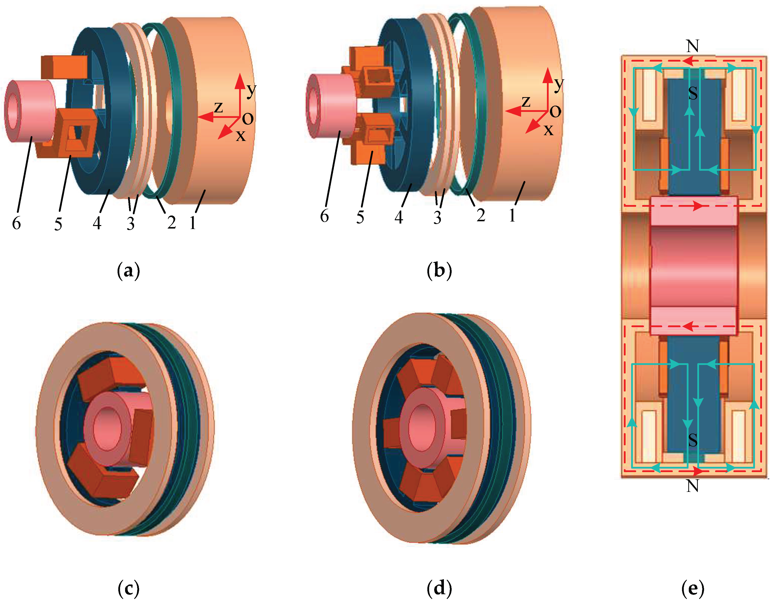
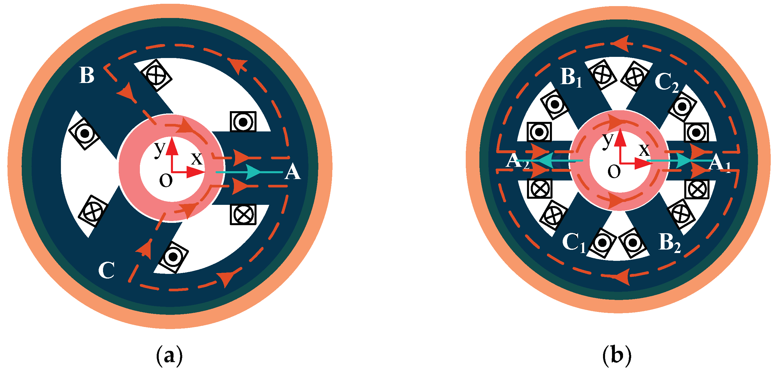
2. Structure and Working Principle of the RAHMBs

Figure 2a,b show the main components of the three-pole and six-pole RAHMB, respectively. After removing the outermost axial stator, the structure of the three-pole and six-pole RAHMBs are shown in Figure 2c,d. The axial magnetic flux path of the RAHMBs are shown in Figure 2e. The radially magnetized permanent magnet ring provides axial- and radial-bias magnetic fluxes at the same time. The differences between Figure 2a,b are the number of the magnetic poles and the radial control coils. In Figure 2 and Figure 3, the green solid lines with arrows indicate the bias of the magnetic fluxes which are generated by a permanent magnet. Starting from the N-pole of the PM, the bias magnetic fluxes are evenly divided into two parts to enter both sides of the axial stator, where they pass through the axial air gap, rotor, and radial air gap, and then are divided into six parts to enter the radial stator, eventually returning to the S-pole of the PM. In Figure 2e, the red dashed lines with arrows indicate the control magnetic fluxes which are generated by the axial control coils, the axial control fluxes form the closed loop between the axial stator, the axial air gap, and the rotor. The radial magnetic flux paths of the three-pole and six-pole RAHMBs are shown in Figure 3a,b, respectively, and the magnetic flux paths of the A-phase are used as examples. In Figure 3, the orange dashed lines with arrows indicate the control magnetic fluxes which are generated by radial control coils. The radial control fluxes form the closed loop between the radial stator, the radial air gap, and the rotor.

The radial stator shown in Figure 3a consists of a circular radial stator yoke and three magnetic poles uniformly distributed along the circumference. Similarly, the radial stator shown in Figure 3b consists of a circular radial stator yoke and six magnetic poles uniformly distributed along the circumference. The control coils are wound on each radial magnetic pole, and the two opposite six-pole coils with the same winding direction are connected in series as one phase; three phases of three-pole and six-pole coils are both connected in a star connection and driven by a three-phase power inverter.

When the rotor starts to suspend, the rotor stays in the equilibrium position under the bias magnetic fluxes. Once the rotor deviates away from the equilibrium position under the external disturbance force, through changing the control currents, the control magnetic flux is superimposed with the bias magnetic flux at the large air gap, and the control magnetic flux is eliminated along with the bias magnetic flux at the small air gap in order to make the rotor bear the force in the opposite direction to the external disturbance force; then, the rotor returns to the equilibrium position.

3. Mathematical Model and Capacity Analysis of the RAHMBs

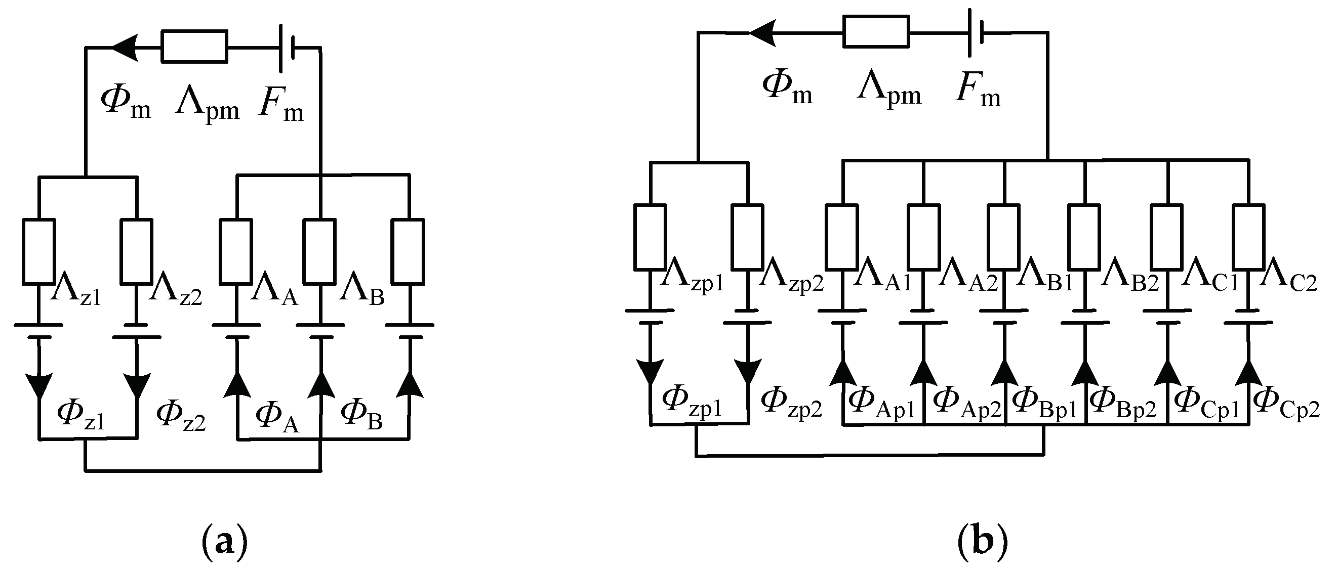
3.1. Magnetic Circuit Analysis

In order to simplify the analysis and create reasonable instructions, the following assumptions are made: the radial width of the radial magnetic pole of the six-pole RAHMB is equal to half that of the three-pole RAHMB, and the other parameters adhere to the same principle. Because the magnetic permeability of the steel materials is infinitely higher than that of the air gap, the reluctance of the steel materials is neglected in the analysis.

In Figure 4, F_m is the magnetomotive force of the PM, Φ_m is the total magnetic flux of the PM, and Λ_pm is the permeance of the PM. Φ_zp1, Φ_zp2, Φ_j, Φ_jp1, and Φ_jp2 (j = A, B, C) are the bias fluxes of each axial and radial air gap, and Λ_z1, Λ_z2, Λ_j, Λ_j1, and Λ_j2 are the magnetic permeances of each axial and radial air gap, respectively. Supposing that the displacement of the rotor deviates away from the equilibrium position, the x, y, and z directions are labeled x, y, and z, respectively.

The magnetic permeances of the PM for each axial and radial air gap are:

$${\mathsf{\Lambda }}_{\mathrm{m}}=\frac{{\mu }_0{\mu }_{\mathrm{r}}{S}_{\mathrm{pm}}}{l_{\mathrm{pm}}}\hspace{0.17em}$$

(1)

$$\{\begin{array}{l}{\mathsf{\Lambda }}_{\mathrm{z}1}={\mathsf{\Lambda }}_{\mathrm{zp}1}=\frac{{\mu }_0{S}_{{z}}}{{\delta }_{{z}}+z}\hspace{0.17em}\\ {\mathsf{\Lambda }}_{\mathrm{z}2}={\mathsf{\Lambda }}_{\mathrm{zp}2}=\frac{{\mu }_0{S}_{{z}}}{{\delta }_{{z}}-z}\end{array}$$

(2)

$$\{\begin{array}{l}{\mathsf{\Lambda }}_{\mathrm{A}}={\mathsf{\Lambda }}_{\mathrm{A}1}=\frac{{\mu }_0{S}_{\mathrm{r}}}{{\delta }_{\mathrm{r}}-x}\hspace{0.17em},{\mathsf{\Lambda }}_{\mathrm{A}2}=\frac{{\mu }_0{S}_{\mathrm{r}}}{{\delta }_{\mathrm{r}}+x}\\ {\mathsf{\Lambda }}_{\mathrm{B}}={\mathsf{\Lambda }}_{\mathrm{B}1}=\frac{{\mu }_0{S}_{\mathrm{r}}}{{\delta }_{\mathrm{r}}+\frac{1}{2}x-\frac{\sqrt{3}}{2}y}\hspace{0.17em},\hspace{0.17em}{\mathsf{\Lambda }}_{\mathrm{B}2}=\frac{{\mu }_0{S}_{\mathrm{r}6}}{{\delta }_{\mathrm{r}}-\frac{1}{2}x+\frac{\sqrt{3}}{2}y}\\ {\mathsf{\Lambda }}_{\mathrm{C}}={\mathsf{\Lambda }}_{\mathrm{C}1}=\frac{{\mu }_0{S}_{\mathrm{r}}}{{\delta }_{\mathrm{r}}+\frac{1}{2}x+\frac{\sqrt{3}}{2}y}\hspace{0.17em},\hspace{0.17em}{\mathsf{\Lambda }}_{\mathrm{C}2}=\frac{{\mu }_0{S}_{\mathrm{r}6}}{{\delta }_{\mathrm{r}}-\frac{1}{2}x-\frac{\sqrt{3}}{2}y}\end{array}$$

(3)

where μ₀ is the vacuum permeability, μ_r is the relative permeability of the PM, S_pm is the average area of inner face and outer face of the PM along the magnetized direction, l_pm is the length of the PM in the magnetized direction, δ_z and δ_r are uniform air-gap lengths of the axial and radial air gap without rotor eccentricity, respectively, S_z and S_r are the area of axial and radial magnetic pole faces, respectively, the value of S_r is set as S_r3 when the magnetic permeances of the radial air gap is Λ_j, the value of S_r is set as S_r6 when the magnetic permeances of the radial air gap is Λ_j1, and S_r3 and S_r6 are the radial-magnetic-pole-face area of the three-pole and six-pole RAHMB, respectively.

3.1.1. Mathematical Model of the Three-Pole RAHMB

Based on Kirchhoff’s Law regarding bias magnetic circuits, the bias magnetic fluxes of each axial and radial air gap are:

$$\{\begin{array}{l}{\Phi }_{\mathrm{z}1}=\frac{{\mathsf{\Lambda }}_{\mathrm{m}}{\mathsf{\Lambda }}_{\mathrm{r}3}{\mathsf{\Lambda }}_{\mathrm{z}1}{F}_{\mathrm{m}}}{{\mathsf{\Lambda }}_{\mathrm{s}3}}+\frac{{\mathsf{\Lambda }}_{\mathrm{z}1}{N}_{\mathrm{z}}{i}_{\mathrm{z}}}{2}\\ {\Phi }_{\mathrm{z}2}=\frac{{\mathsf{\Lambda }}_{\mathrm{m}}{\mathsf{\Lambda }}_{\mathrm{r}3}{\mathsf{\Lambda }}_{\mathrm{z}2}{F}_{\mathrm{m}}}{{\mathsf{\Lambda }}_{\mathrm{s}3}}-\frac{{\mathsf{\Lambda }}_{\mathrm{z}2}{N}_{\mathrm{z}}{i}_{\mathrm{z}}}{2}\\ {\Phi }_j=\frac{{\mathsf{\Lambda }}_{\mathrm{m}}{\mathsf{\Lambda }}_{\mathrm{a}}{\mathsf{\Lambda }}_j{F}_{\mathrm{m}}}{{\mathsf{\Lambda }}_{\mathrm{s}3}}+{\mathsf{\Lambda }}_j{N}_{\mathrm{r}}{i}_j\end{array}$$

(4)

where N_zi_x and N_ri_j describe the magnetomotive force generated by axial and radial control coils, Λ_r3 = Λ_A + Λ_B + Λ_C, Λ_a = Λ_z1 + vΛ_z2, and Λ_s3 = Λ_r3Λ_a + Λ_mΛ_a + Λ_mΛ_r3.

According to the relationship between the magnetic force and the magnetic fluxes, the axial and radial magnetic suspension forces can be expressed as:

$$\{\begin{array}{l}{F}_{3\mathrm{z}}=F_{\mathrm{z}1}-F_{\mathrm{z}2}=\frac{{\Phi }_{\mathrm{z}1}^2-{\Phi }_{\mathrm{z}2}^2}{2{\mu }_0{S}_{\mathrm{z}}}\\ F_{3x}=F_{\mathrm{A}}-\frac{1}{2}\left(F_{\mathrm{B}}+F_{\mathrm{C}}\right)=\frac{2{\Phi }_{\mathrm{A}}^2-{\Phi }_{\mathrm{B}}^2-{\Phi }_{\mathrm{C}}^2}{4{\mu }_0{S}_{\mathrm{r}3}}\\ F_{3\mathrm{y}}=\frac{\sqrt{3}}{2}\left(F_{\mathrm{B}}-F_{\mathrm{C}}\right)=\frac{\sqrt{3}\left({\Phi }_{\mathrm{B}}^2-{\Phi }_{\mathrm{C}}^2\right)}{4{\mu }_0{S}_{\mathrm{r}3}}\end{array}$$

(5)

3.1.2. Mathematical Model of the Six-Pole RAHMB

Based on Kirchhoff’s Law regarding bias magnetic circuits, the bias magnetic fluxes of each axial and radial air gap are:

$$\{\begin{array}{l}{\Phi }_{\mathrm{zp}1}=\frac{{\mathsf{\Lambda }}_m{\mathsf{\Lambda }}_{\mathrm{r}6}{\mathsf{\Lambda }}_{\mathrm{zp}1}{F}_m}{{\mathsf{\Lambda }}_{s6}}+\frac{{\mathsf{\Lambda }}_{\mathrm{zp}1}{N}_{\mathrm{z}}{i}_{\mathrm{z}}}{2}\\ {\Phi }_{\mathrm{zp}2}=\frac{{\mathsf{\Lambda }}_m{\mathsf{\Lambda }}_{\mathrm{r}6}{\mathsf{\Lambda }}_{\mathrm{zp}2}{F}_m}{{\mathsf{\Lambda }}_{s6}}-\frac{{\mathsf{\Lambda }}_{\mathrm{zp}2}{N}_{\mathrm{z}}{i}_{\mathrm{z}}}{2}\\ {\Phi }_{j\mathrm{p}1}=\frac{{\mathsf{\Lambda }}_m{\mathsf{\Lambda }}_{\mathrm{a}}{\mathsf{\Lambda }}_{j\mathrm{p}1}{F}_m}{{\mathsf{\Lambda }}_{s6}}+\frac{{\mathsf{\Lambda }}_{j\mathrm{p}1}{N}_{\mathrm{r}}{i}_j}{2}\\ {\Phi }_{j\mathrm{p}2}=\frac{{\mathsf{\Lambda }}_m{\mathsf{\Lambda }}_{\mathrm{a}}{\mathsf{\Lambda }}_{j\mathrm{p}2}{F}_m}{{\mathsf{\Lambda }}_{s6}}-\frac{{\mathsf{\Lambda }}_{j\mathrm{p}2}{N}_{\mathrm{z}}{i}_{\mathrm{z}}}{2}\end{array}$$

(6)

where Λ_r6 = Λ_A1 + Λ_A2 + Λ_B1 + Λ_B2 + Λ_C1 + Λ_C2 and Λ_s6 = Λ_r6Λ_a + Λ_mΛ_a + Λ_mΛ_r6.

According to the relationship between the magnetic force and the magnetic fluxes, the axial and radial magnetic suspension forces can be expressed as:

$$\{\begin{array}{l}{F}_{6\mathrm{z}}=F_{\mathrm{zp}1}-F_{\mathrm{zp}2}=\frac{{\Phi }_{\mathrm{zp}1}^2-{\Phi }_{\mathrm{zp}2}^2}{2{\mu }_0{S}_{\mathrm{z}}}\\ F_{6x}=F_{\mathrm{A}1}-F_{\mathrm{A}2}-\frac{\left(F_{\mathrm{B}1}-F_{\mathrm{B}2}-F_{\mathrm{C}1}+F_{\mathrm{C}2}\right)}{2}=\frac{2{\Phi }_{\mathrm{Ap}1}^2-2{\Phi }_{\mathrm{Ap}2}^2-\left({\Phi }_{\mathrm{Bp}1}^2-{\Phi }_{\mathrm{Bp}2}^2-{\Phi }_{\mathrm{Cp}1}^2+{\Phi }_{\mathrm{Cp}2}^2\right)}{4{\mu }_0{S}_{\mathrm{r}6}}\\ F_{6\mathrm{y}}=\frac{\sqrt{3}}{2}\left(F_{\mathrm{B}1}-F_{\mathrm{B}2}-F_{\mathrm{C}1}+F_{\mathrm{C}2}\right)=\frac{\sqrt{3}\left({\Phi }_B^2-{\Phi }_C^2\right)}{4{\mu }_0{S}_{\mathrm{r}6}}\end{array}$$

(7)

3.2. Analysis of the Radial Capacity

In Equations (5) and (7), the expressions of the axial suspension forces are same, and the expressions of the radial suspension forces are strikingly different, so the maximum radial capacities of the three-pole and six-pole RAHMBs were analyzed.

3.2.1. The Maximum Radial Capacity of the Three-Pole RAHMB

The radial capacity of the RAHMB is limited by the saturated flux density of the magnetic pole. In order to avoid magnetic saturation in the magnetic pole, it was assumed that when the flux in the air gap reaches the set saturated flux density B_S, the value of the control current is at its maximum, and the suspension force under this air gap is the largest. Take the maximum suspension force in the x-positive direction as an example.

When the positive maximum control current i_rmax is injected into A-phase, the flux density in the air gap under the A-pole reaches B_S, and the flux in the air gap under the A-pole is:

$${\Phi }_{3\mathrm{A}}={\Phi }_{3\mathrm{r}0}+{\Phi }_{3\mathrm{r}\mathrm{c}}=B_{\mathrm{S}}{S}_{\mathrm{r}3}$$

(8)

where Φ_3A is the flux of the A-pole air gap, Φ_3r0 is the bias flux of the air gap, and Φ_3rc is the control flux of the air gap, whose value is N_r3i_j/Λ_3r0.

When the negative maximum control current −i_rmax is injected into A-phase, the flux in the air gap under the A-pole is nearly 0, which can be expressed as:

$${\Phi }_{3\mathrm{A}}={\Phi }_{3\mathrm{r}0}-{\Phi }_{3\mathrm{r}\mathrm{c}}=0$$

(9)

Then, the expression of Φ_3rc is:

$${\Phi }_{3\mathrm{r}\mathrm{c}}=\frac{{\mu }_0{N}_{\mathrm{r}3}{i}_{\mathrm{rmax}}{S}_{\mathrm{r}3}}{{\delta }_{\mathrm{r}}}=\frac{B_{\mathrm{S}}{S}_{\mathrm{r}3}}{2}$$

(10)

Because the MB is driven by a three-phase power inverter, with the limitation of the sum of the three-phase current being zero, when the positive maximum control current i_rmax is injected into A-phase, in order to produce the maximum suspension force, the control currents −0.5i_rmax are injected into B- and C-phase, and the fluxes in the air gap under the B- and C-pole are:

$${\Phi }_{3\mathrm{B}}={\Phi }_{3\mathrm{C}}={\Phi }_{3\mathrm{r}0}-\frac{{\Phi }_{3\mathrm{r}\mathrm{c}}}{2}=\frac{B_{\mathrm{S}}{S}_{\mathrm{r}3}}{4}$$

(11)

At this time, the maximum suspension force F_3xmax is produced in the x-positive direction as:

$$F_{3\mathrm{x}\mathrm{m}\mathrm{a}\mathrm{x}}=F_{\mathrm{A}}-\frac{1}{2}\left(F_{\mathrm{B}}+F_{\mathrm{C}}\right)=\frac{15B_{\mathrm{S}}{}^2{S}_{r3}}{32{\mu }_0}$$

(12)

When the negative maximum control current −i_rmax is injected into A-phase, the control currents 0.5i_rmax are injected into B- and C-phase, and the fluxes in the air gap under the B- and C-pole are:

$${\Phi }_{3\mathrm{B}}={\Phi }_{3\mathrm{C}}={\Phi }_{3\mathrm{r}0}+\frac{{\Phi }_{3\mathrm{r}\mathrm{c}}}{2}=\frac{3B_{\mathrm{S}}{S}_{\mathrm{r}3}}{4}$$

(13)

At this time, the maximum suspension force F_3xmax is produced in the x-negative direction as:

$$F_{3\mathrm{x}\mathrm{m}\mathrm{a}\mathrm{x}}=F_{3\mathrm{A}}-\frac{1}{2}\left(F_{3\mathrm{B}}+F_{3\mathrm{C}}\right)=-\frac{9B_{\mathrm{S}}{}^2{S}_{\mathrm{r}3}}{32{\mu }_0}$$

(14)

When the positive maximum control current i_rmax is injected into B-phase, the negative maximum control current −i_rmax is injected into C-phase, and the control current 0 is injected into A-phase; therefore, the maximum suspension force F_3ymax is produced in the y-positive direction as:

$$F_{3\mathrm{y}\mathrm{m}\mathrm{a}\mathrm{x}}=\frac{\sqrt{3}}{2}\left(F_{3\mathrm{B}}-F_{3\mathrm{C}}\right)=\frac{\sqrt{3}{B}_{\mathrm{S}}{}^2{S}_{\mathrm{r}3}}{4{\mu }_0}$$

(15)

3.2.2. The Maximum Radial Capacity of the Six-Pole RAHMB

Different from the three-pole RAHMB, the structure of the six-pole RAHMB is symmetrical; it has the same suspension force in the x-positive and -negative directions. When the positive maximum control current i_rmax is injected into A-phase, the control currents −0.5i_rmax are injected into the B- and C-phase, and the fluxes in the air gap under each magnetic pole are:

$$\{\begin{array}{l}{\Phi }_{6\mathrm{A}1}={\Phi }_{6\mathrm{r}0}+{\Phi }_{6\mathrm{r}\mathrm{c}}=B_{\mathrm{S}}{S}_{\mathrm{r}6}\\ {\Phi }_{6\mathrm{A}2}={\Phi }_{6\mathrm{r}0}-{\Phi }_{6\mathrm{r}\mathrm{c}}=0\\ {\Phi }_{6\mathrm{B}1}={\Phi }_{6\mathrm{C}2}={\Phi }_{6\mathrm{r}0}-\frac{{\Phi }_{6\mathrm{r}\mathrm{c}}}{2}=\frac{B_{\mathrm{S}}{S}_{\mathrm{r}6}}{4}\\ {\Phi }_{6\mathrm{B}2}={\Phi }_{6\mathrm{C}1}={\Phi }_{6\mathrm{r}0}+\frac{{\Phi }_{6\mathrm{r}\mathrm{c}}}{2}=\frac{3B_{\mathrm{S}}{S}_{\mathrm{r}6}}{4}\end{array}$$

(16)

where Φ_6jh (h = 1, 2) is the flux of the corresponding air gap, Φ_6r0 is the bias flux of the air gap, and Φ_6rc is the control flux of the air gap.

At this time, the maximum suspension force F_6xmax is produced in the x-positive direction as:

$$F_{6\mathrm{x}\mathrm{m}\mathrm{a}\mathrm{x}}=F_{6\mathrm{A}1}-F_{6\mathrm{A}2}-\frac{1}{2}\left(F_{6\mathrm{B}1}-F_{6\mathrm{B}2}-F_{6\mathrm{C}1}+F_{6\mathrm{C}2}\right)=\frac{3B_{\mathrm{S}}{}^2{S}_{\mathrm{r}6}}{4{\mu }_0}$$

(17)

When the positive maximum control current i_rmax is injected into B-phase, the negative maximum control current −i_rmax is injected into C-phase, and the control current 0 is injected into A-phase; therefore, the maximum suspension force F_6ymax is produced in the y-positive direction as:

$$F_{6\mathrm{y}\mathrm{m}\mathrm{a}\mathrm{x}}=\frac{\sqrt{3}}{2}\left(F_{6\mathrm{B}1}-F_{6\mathrm{B}2}+F_{6\mathrm{C}1}-F_{6\mathrm{C}2}\right)=\frac{\sqrt{3}{B}_{\mathrm{S}}{}^2{S}_{\mathrm{r}6}}{2{\mu }_0}$$

(18)

From Equations (12), (14) and (15), the radial suspension forces of the three-pole RAHMB are different in the x and y directions, and they are also different in the x-positive and -negative directions because of the asymmetric structure. Since the maximum capacity of the MB depends on the smallest value of the maximum suspension force in each direction, the suspension force of the three-pole RAHMB in the x-negative direction was taken as the radial capacity. From Equations (17) and (18), the suspension force of the six-pole RAHMB in the x direction was taken as the radial capacity.

4. Simulation Validations

In order to verify the validity of the above analysis, 3-D FEM models of the three-pole and six-pole RAHMBs were built using the ANSYS software. In Equations (5) and (7), the axial and radial suspension forces are nonlinear functions of the displacements and the control currents. Through changing the displacements and the control currents, the nonlinearity and the couplings between the degrees of freedom can be analyzed. Because of the limitations of the auxiliary bearing, the displacement changes within the range [−0.25 mm, 0.25 mm] and the maximum control current is 1 A.

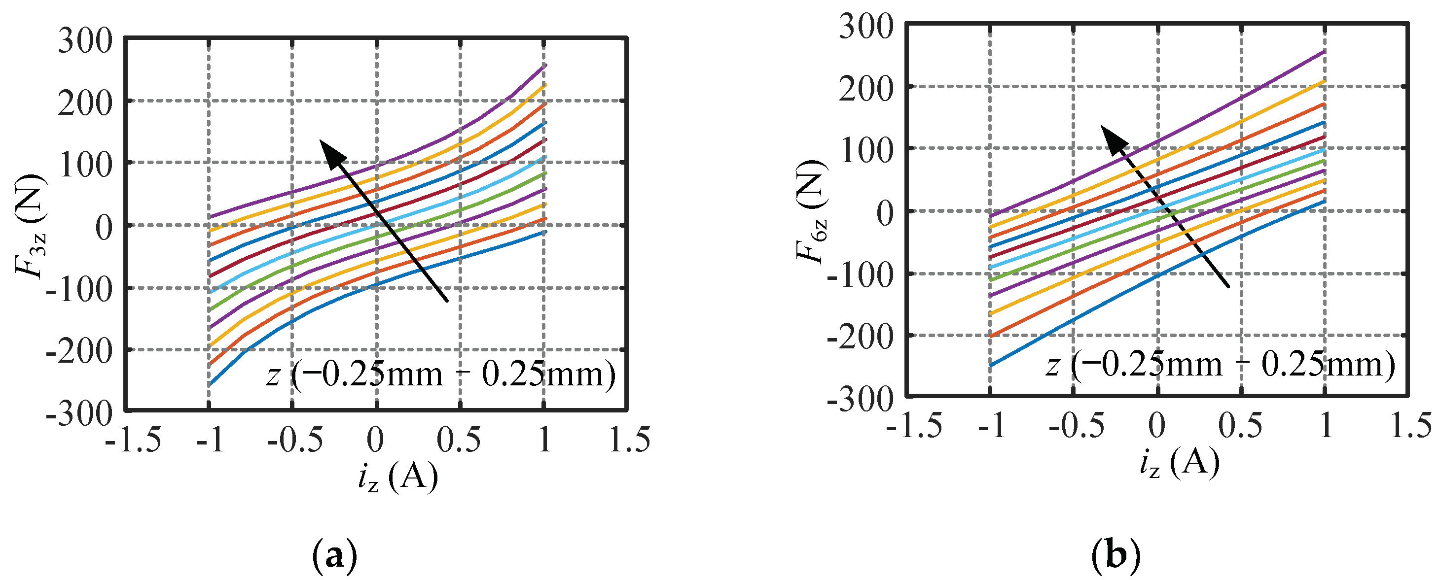
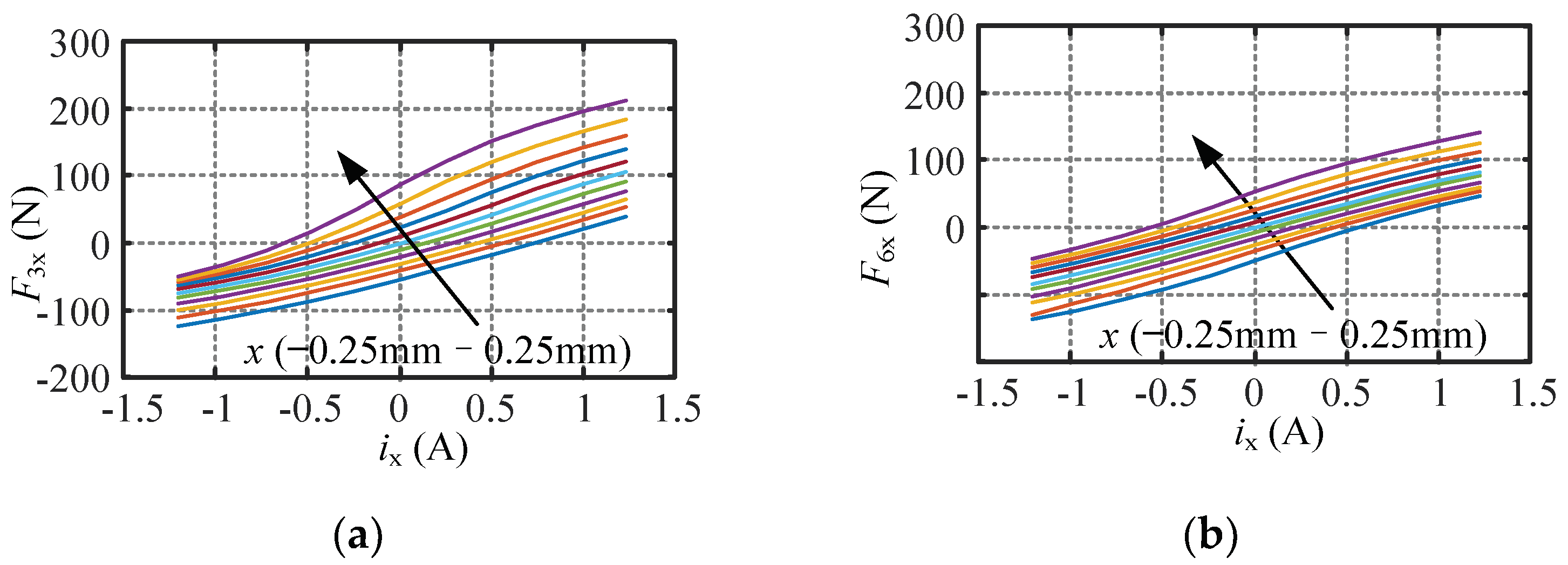
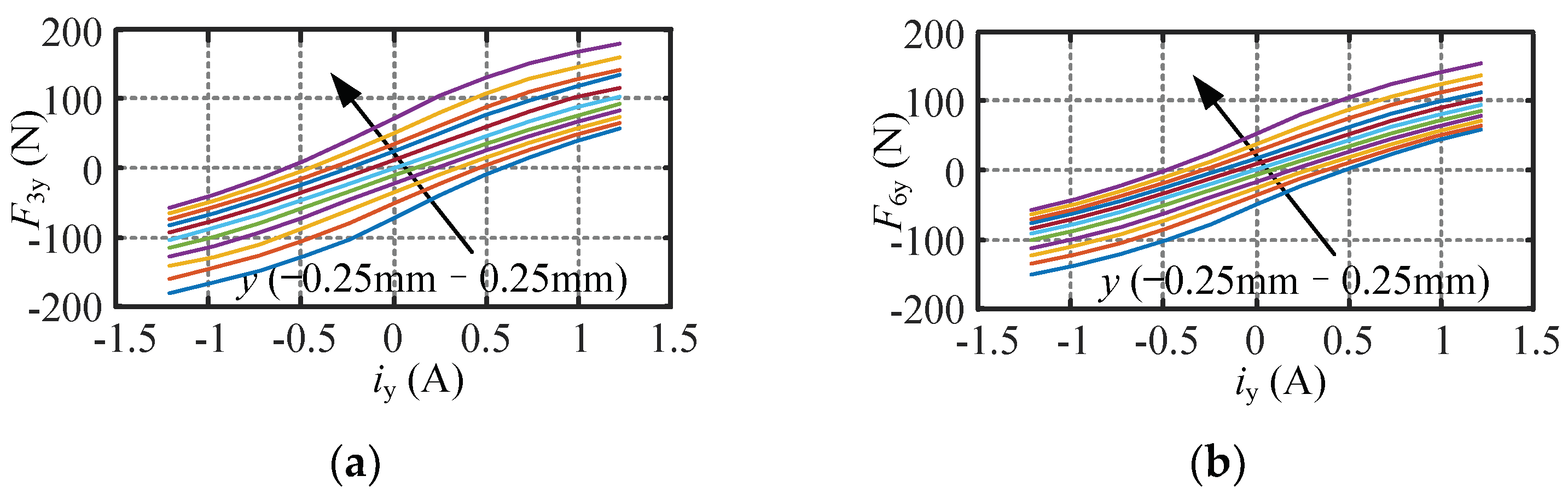
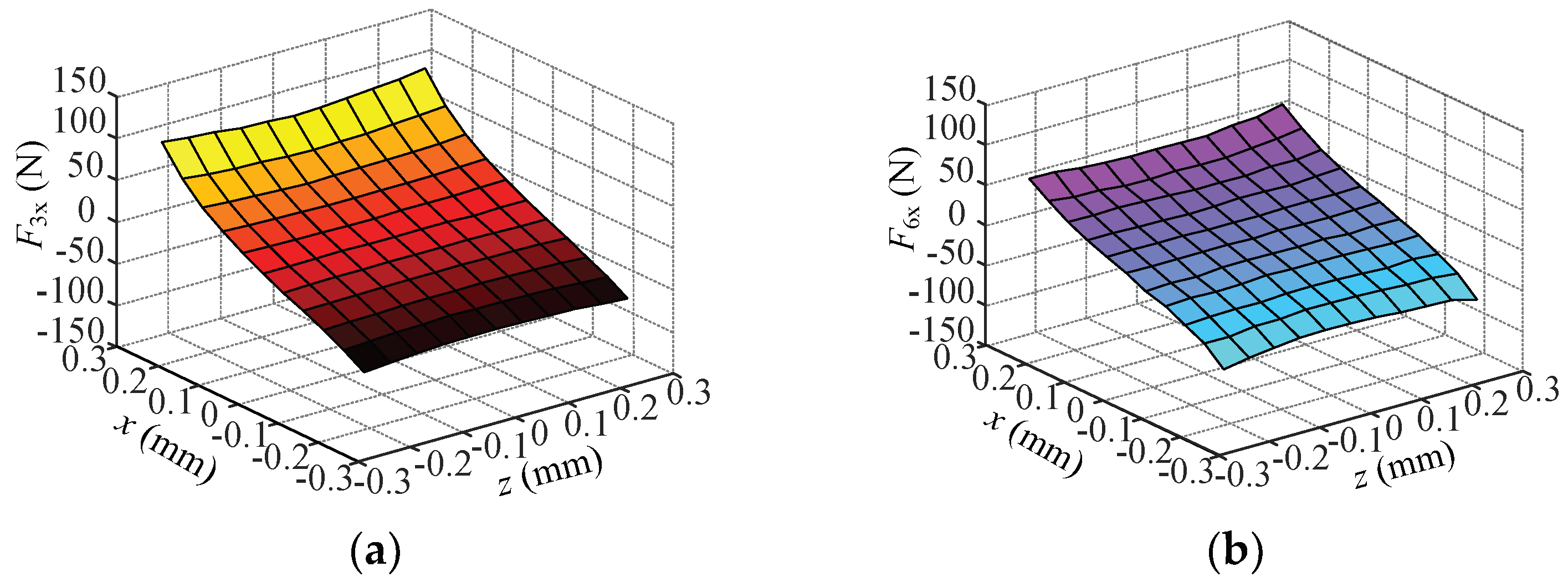
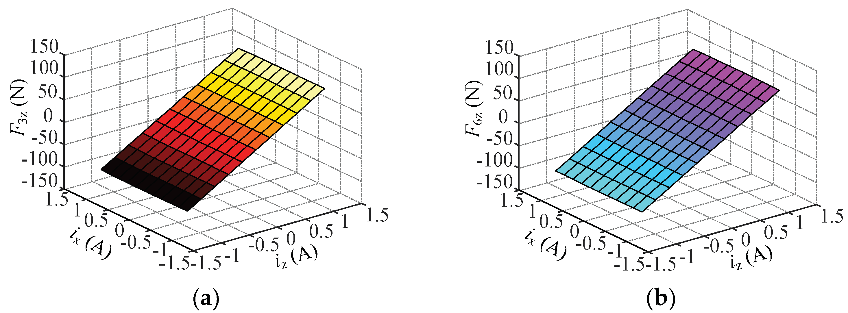
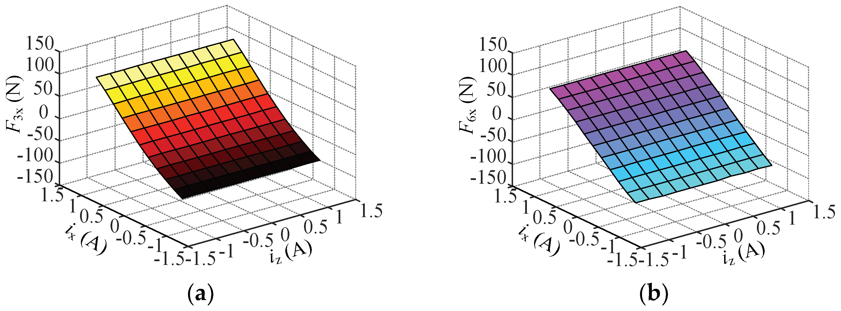
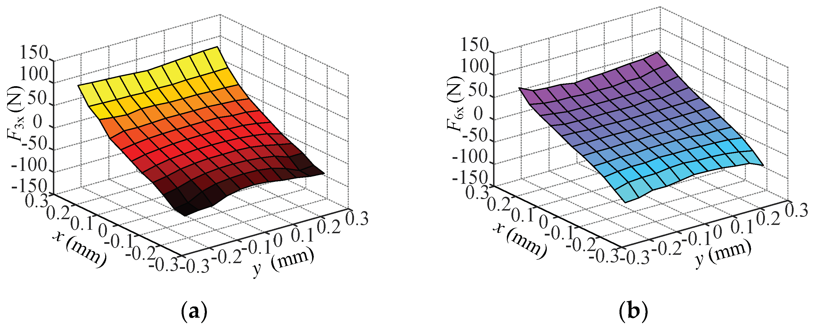
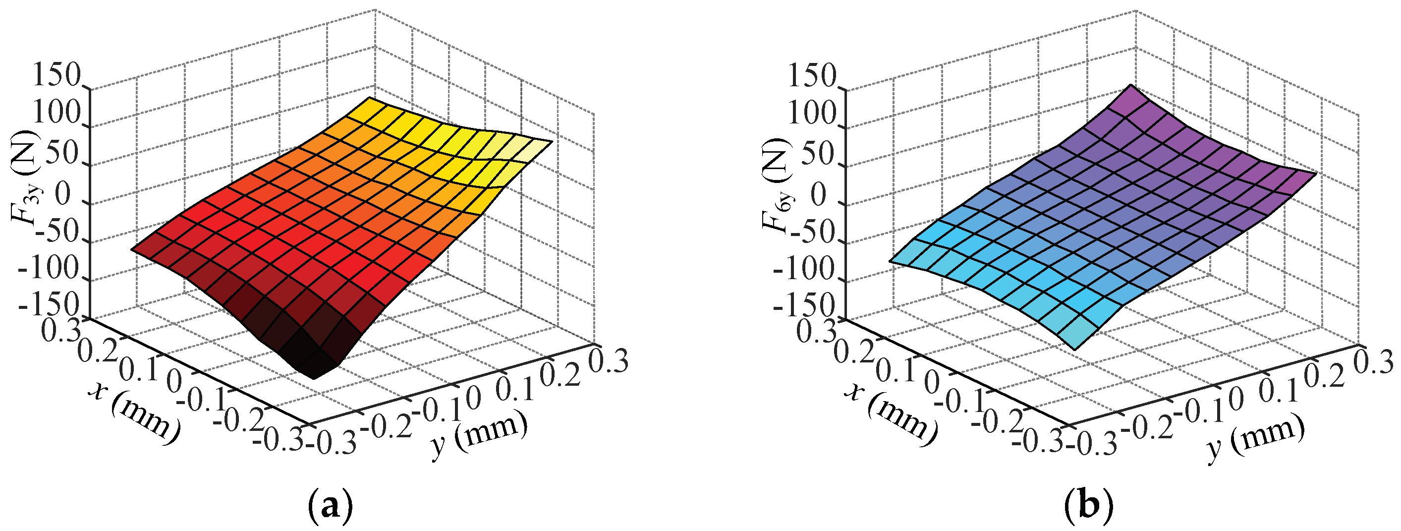
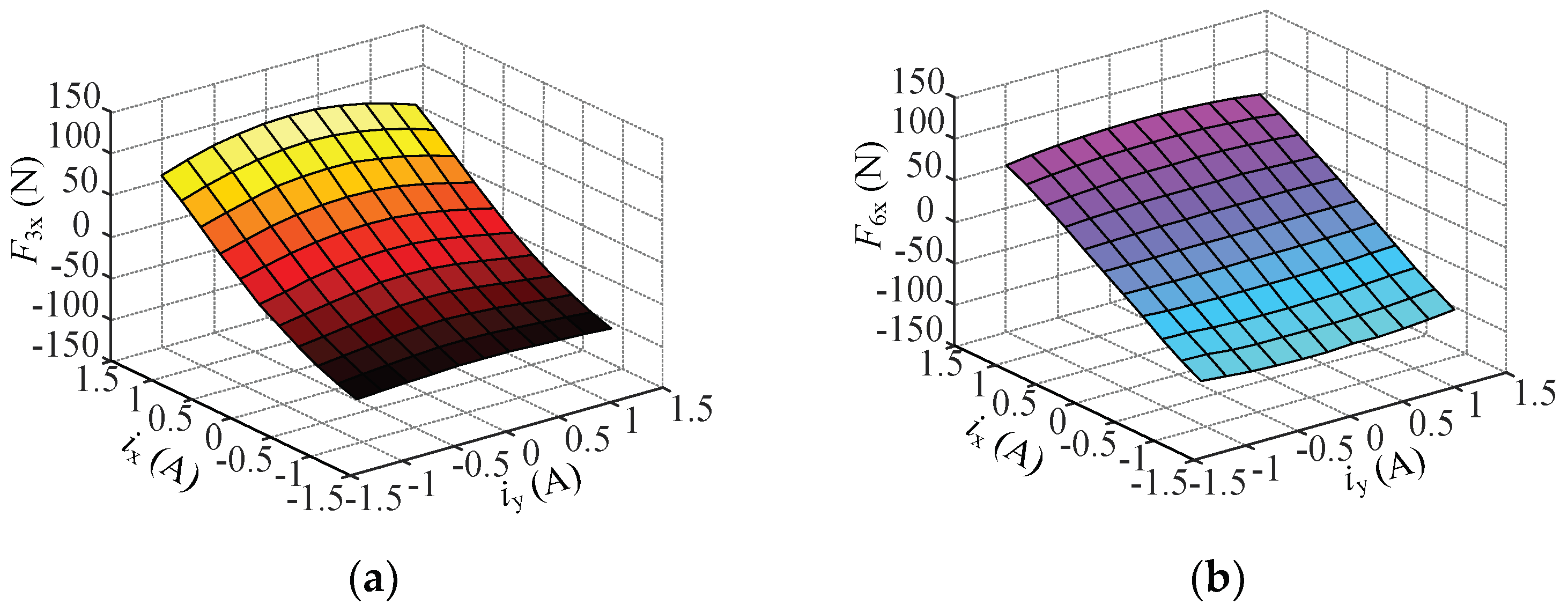
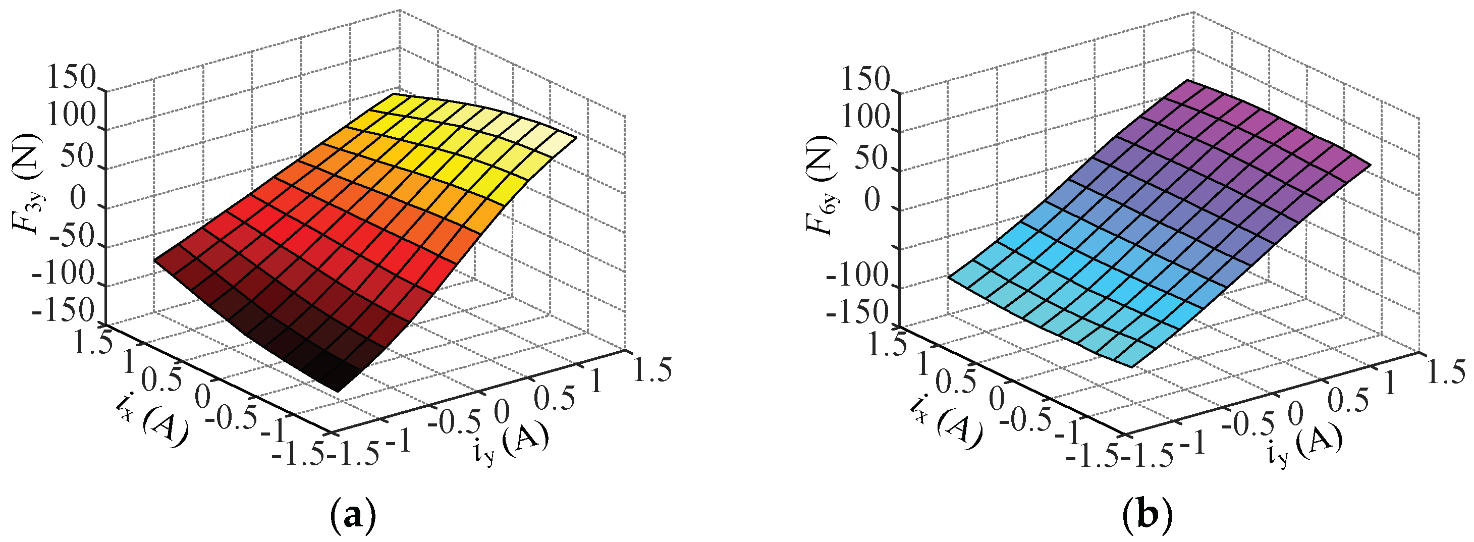
4.1. Nonlinearity Analysis of the Suspension Force

The waveforms of the suspension forces with the corresponding control currents and displacements are shown in Figure 5, Figure 6 and Figure 7.

As seen in Figure 5, when the values of the axial control current i_z and axial displacement z change around 0, both values of the axial suspension force of the three-pole and six-pole RAHMBs change linearly. With the values of the axial control current i_z and displacement z trending towards a maximum or minimum, compared with the change in the axial suspension force F_3z, the change in F_6z is more linear.

As seen in Figure 6 and Figure 7, the linearity near the equilibrium position is still ideal. With the values of the radial control current i_x (i_y) and displacement x (y) trending towards a maximum or minimum, compared with the change in radial suspension force F_3x (F_3y), the change in F_6x (F_6y) is also more linear. In Figure 5, Figure 6 and Figure 7 when in the equilibrium position, except Figure 5a, the waveforms are all symmetric around the origin point. The reason for the asymmetric waveform in Figure 6a is the asymmetric distribution of the three magnetic poles along the y axis. Therefore, the linearity of the suspension forces F_6x and F_6y with the corresponding control currents and displacements is better than the linearity of the suspension forces F_3x and F_3y with the corresponding control currents and displacements.

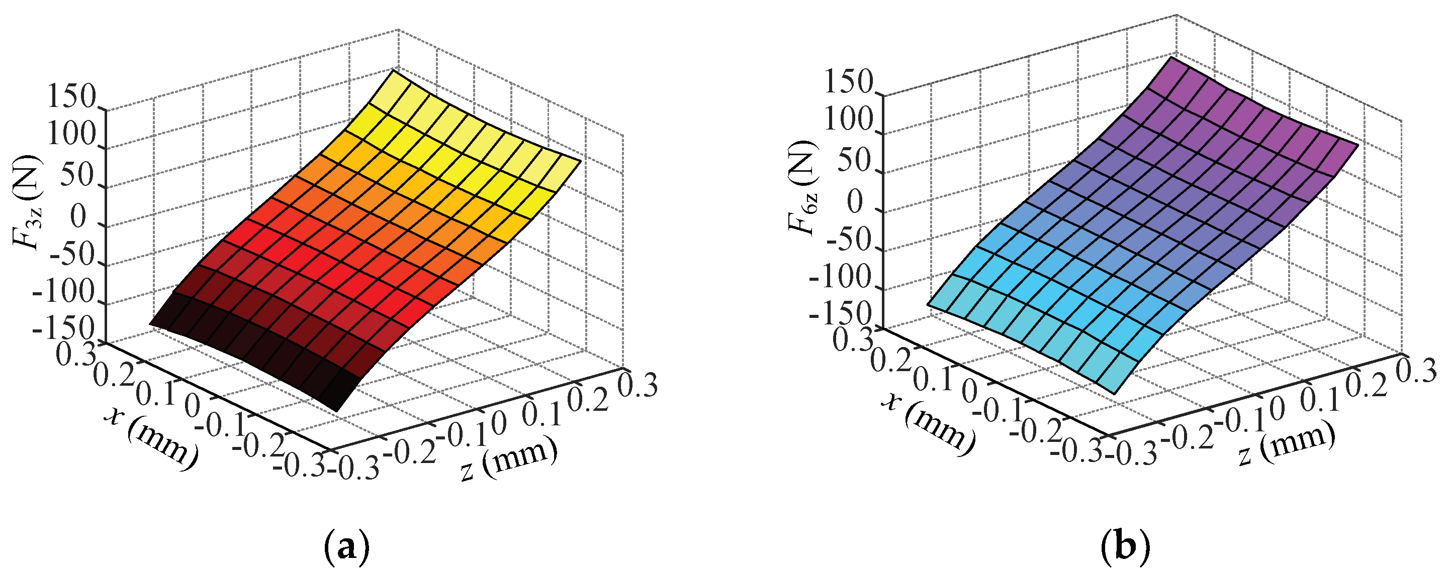
4.2. Coupling Analysis of the Suspension Force

The waveforms of the axial and radial suspension forces with the axial displacement z and the radial displacement x are shown in Figure 8 and Figure 9. In Figure 8, when the radial displacement x changes within the range [−0.25 mm, 0.25 mm], either in the three-pole or six-pole RAHMB, the change in the radial displacement x has little effect on the axial suspension force F_z. In Figure 9, when the axial displacement z changes within the range [−0.25 mm, 0.25 mm], either in the three-pole or six-pole RAHMB, the change in the axial displacement z has little effect on the radial suspension force F_x. Therefore, when the displacement changes within the range, there is nearly no coupling between the axial displacement z and radial displacement x.

The waveforms of the axial and radial suspension forces with the axial control current i_z and the radial control current i_x are shown in Figure 10 and Figure 11. In Figure 10, in both the three-pole and six-pole RAHMB, the change in the radial control current i_x has little effect on the axial suspension force F_z. In Figure 11, in both the three-pole and six-pole RAHMB, the change in the axial control current i_z has little effect on the radial suspension force F_x. Therefore, the magnetic fluxes produced by the axial and radial control currents are independent of each other, which means there is no coupling between axial control current i_z and radial control current i_x.

The waveforms of the radial suspension forces with the radial displacement x and y are shown in Figure 12 and Figure 13. In Figure 12b, the minimum and maximum radial suspension forces of the six-pole RAHMB are 49.5 N and 53.3 N, which are almost equal to each other, while the maximum radial suspension force of 87.7 N for the three-pole RAHMB is bigger than the six-pole RAHMB’s minimum radial suspension force, 53.5 N, as shown in 12a, which is caused by the asymmetric distribution of the three magnetic poles along the y axis. The asymmetric structure of the radial displacement y also has a big influence on the radial suspension force F_3x, as can be seen in Figure 13a. In Figure 12a,b and Figure 13b, compared with the influence of the radial displacement x on the radial suspension force F_6y and the influence of the radial displacement y on the radial suspension force F_6x, the influence of the radial displacement y on the radial suspension force F_3x is bigger, which means that the couplings between the radial displacement x and radial displacement y of the three-pole RAHMB are bigger than the couplings between the radial displacement x and radial displacement y of the six-pole RAHMB.

The waveforms of the radial suspension forces with the radial control currents i_x and i_y are shown in Figure 14 and Figure 15. Because of the asymmetric distribution of the three magnetic poles along the y axis, the influence of the radial control current i_x on the radial suspension force F_3y is bigger than the influence of the radial control current i_y on the radial suspension force F_3x, and it is also bigger than the influence of the radial control current i_y on the radial suspension force F_6x and the radial control current i_x on the radial suspension force F_6y, which means that the couplings between the radial control current i_x and radial control current i_y of the three-pole RAHMB are bigger than the couplings between the radial control current i_x and radial control current i_y of the six-pole RAHMB.

As seen in Figure 8, Figure 9, Figure 10 and Figure 11 for both the three-pole and six-pole RAHMB, there are nearly no couplings between the axial variable and the radial variable. As seen in Figure 12, Figure 13, Figure 14 and Figure 15 the couplings between the radial variables of the three-pole RAHMB are bigger than the couplings between the radial variables of the six-pole RAHMB. The strong couplings between the radial variables of the three-pole RAHMB are caused by the asymmetric distribution of the three magnetic poles along the y axis.

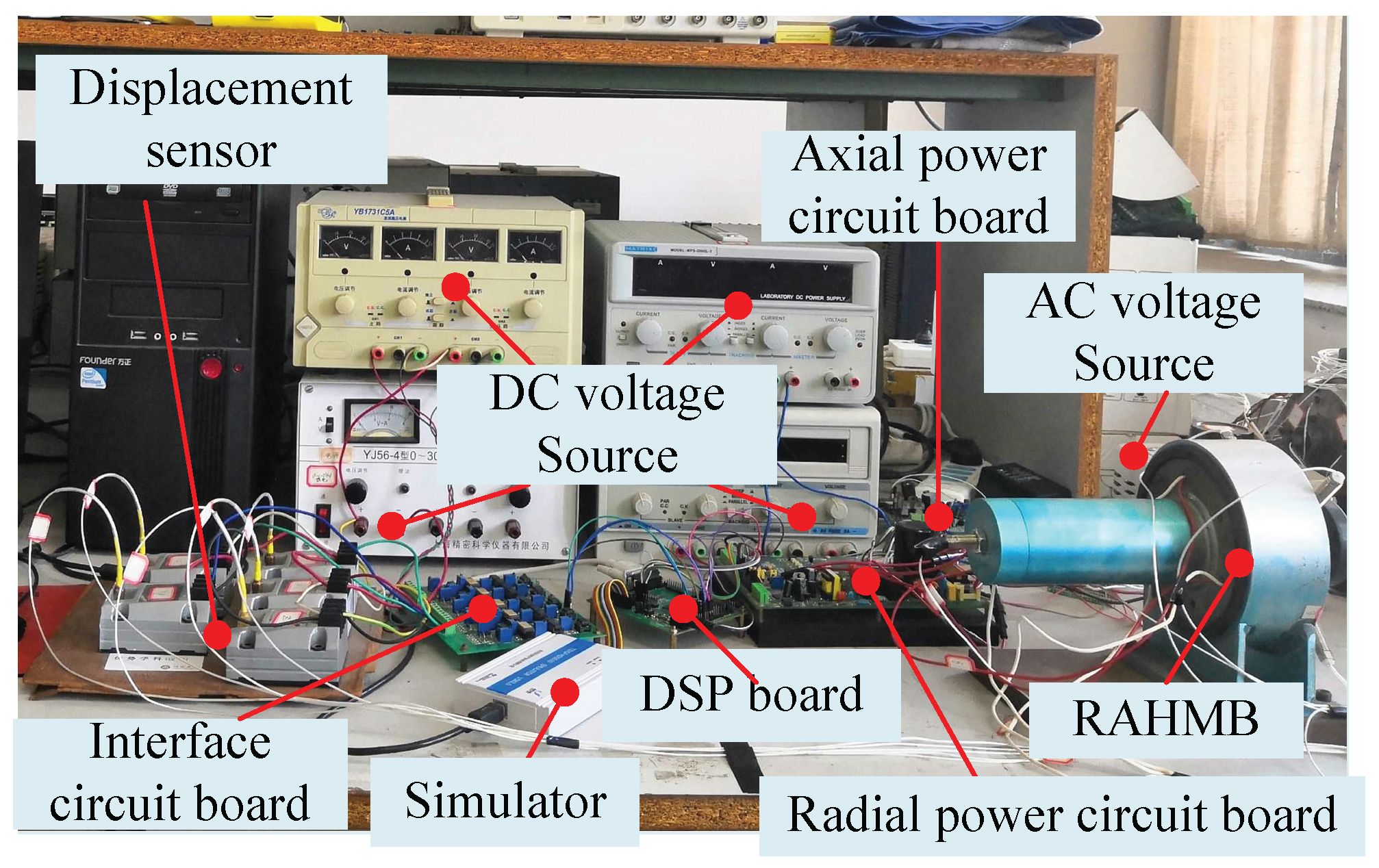
5. Experiment Validations

In order to verify the correctness of the simulation results and further analyze the electromagnetic characteristics of the three-pole and six-pole RAHMBs, the experiment platform of the RAHMBs is shown in Figure 16.

As shown in Figure 16, when the rotor deviated away from the equilibrium position, the offset of the rotor was measured by the displacement sensor; then, the displacement signals were converted into voltage signals and transmitted to the interface circuit. The interface circuit processed the voltage signals within the range of 0–3 V and transmitted them to DSP. In DSP, the signals were compared with the given reference values, the difference signals were put into the controller, and then the controller output the control reference currents. The radial control reference currents were transmitted to the radial power circuit to obtain the radial control current to drive the radial control coils. The axial control reference currents were transmitted to the axial power circuit to obtain the axial control current to drive the axial control coils. By adjusting the control currents, the rotor was returned to the equilibrium position.

5.1. Radial Capacity Validation Experiment

When the control current of 1 A was injected into A-phase coils, and the control current of −0.5 A was injected into B- and C-phase, the rotor was attracted to the auxiliary bearing in the positive direction of the x axis under the action of Maxwell force; the Maxwell force is produced by the PM and control current. A spring dynamometer was used to drag the rotor along the negative direction of the x axis and record the measured value, named force 1, when the rotor moved. Secondly, the rotor was moved to the auxiliary bearing in the positive direction of the x axis without any control current, and we used a spring dynamometer to drag the rotor along the negative direction of the x axis. We recorded the measured value, named force 2; force 2 is the Maxwell force produced by the PM. Thirdly, by subtracting force 2 from force 1, the approximate maximum suspension force produced by the control current was obtained. The simulation and experiment results of the radial capacity in each direction of the three-pole and six-pole RAHMBs are listed in

Table 1. Maximum Suspension Force.

Direction	Three-Pole Maximum Suspension Force (N)		Six-Pole Maximum Suspension Force (N)
	Simulation	Experiment	Simulation	Experiment
Positive x	105.7	121.3	83.8	95.4
Negative x	74.6	84.1	83.6	94.8
y	101.8	114.7	92.1	104.6

.

From Table 1, because the maximum force capacity of the MB depends on the smallest value of the maximum suspension force in each direction, compared with the radial capacity of 84.1 N of the three-pole RAHMB obtained by experiment, the radial capacity of 94.8 N of the six-pole RAHMB is 12.7% greater. The experiment results are similar to the simulation results, which proves the correctness of the theoretical analysis.

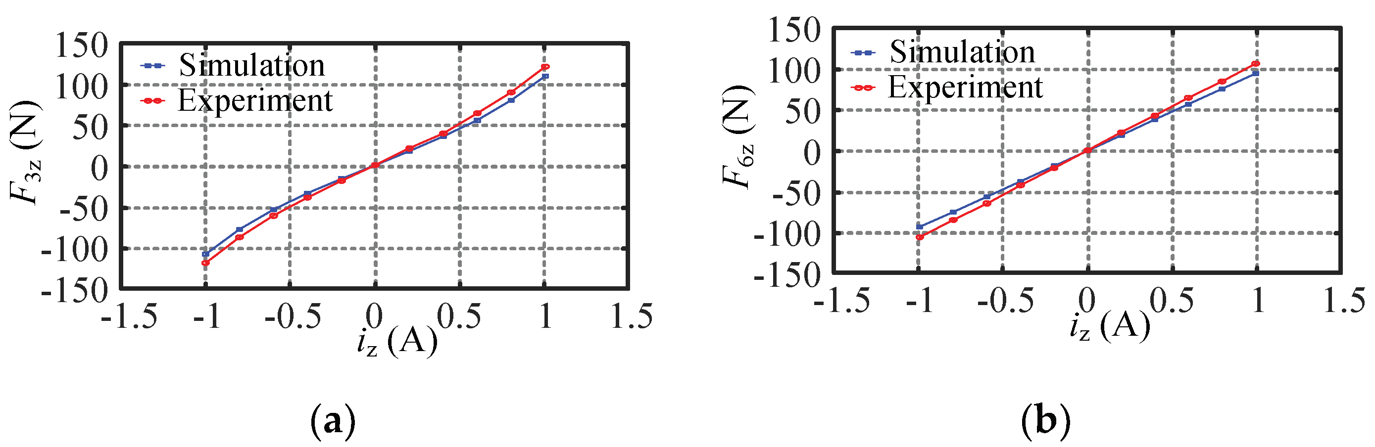
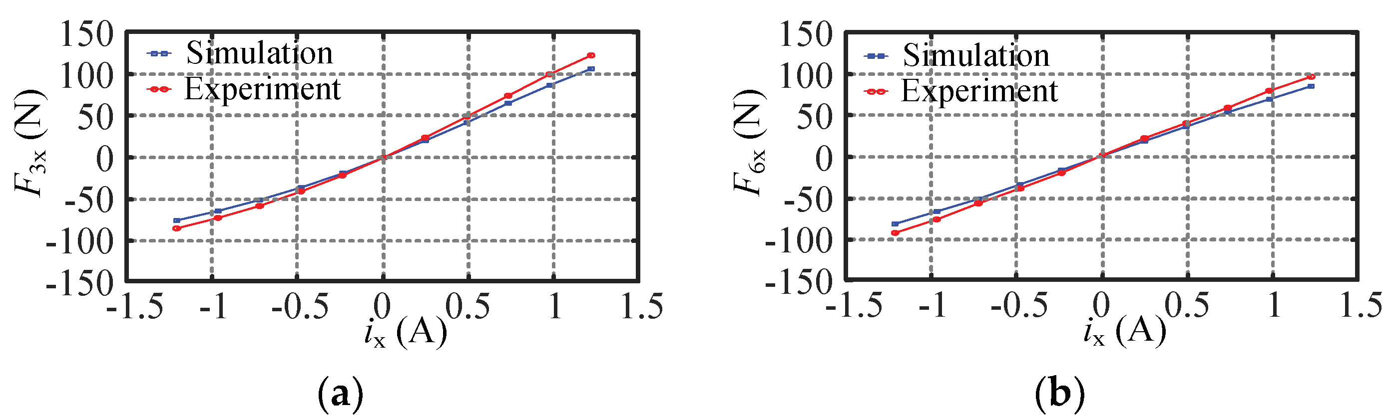
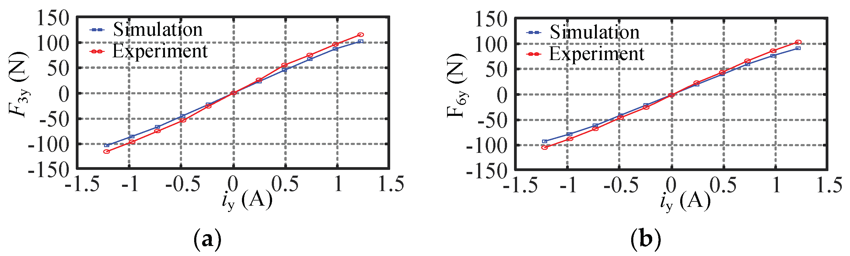
5.2. Nonlinearity Validation Experiment

In order to analyze the nonlinear relationship between the suspension forces with the corresponding control currents, based on the method used in the radial capacity validation experiment, we reduced the control current in A-phase gradually and ensured that the value of the control current in B- and C-phase was equal to the negative half of A-phase, and repeated the above steps. The waveforms between the suspension force and control current in the z, x, and y direction were obtained as shown in Figure 17, Figure 18 and Figure 19. As shown in the figures, the simulation and experiment results are in good agreement, which proves the correctness of the theoretical analysis. Compared with the three-pole RAHMB waveforms, with the control current change, the six-pole RAHMB waveforms changed more linearly, which means that the symmetric distribution of the six magnetic poles reduces the nonlinearity.

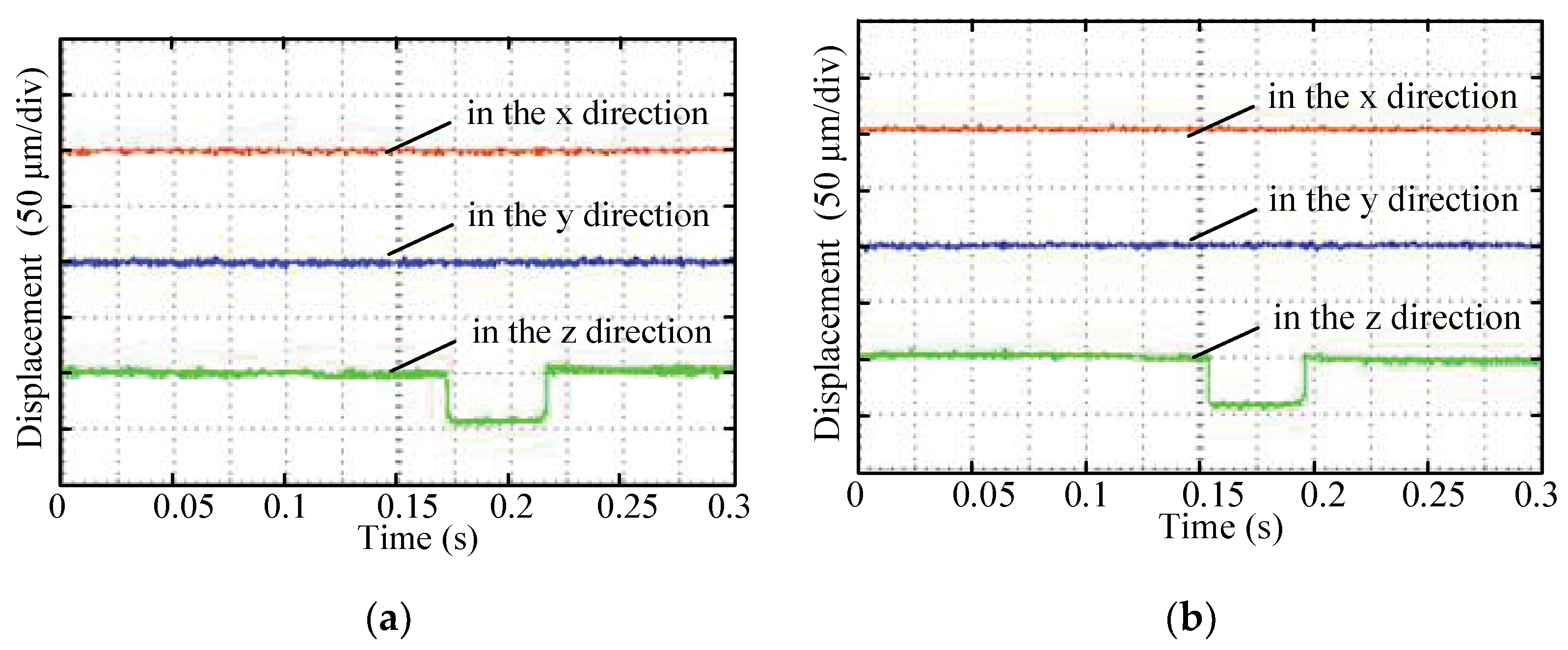
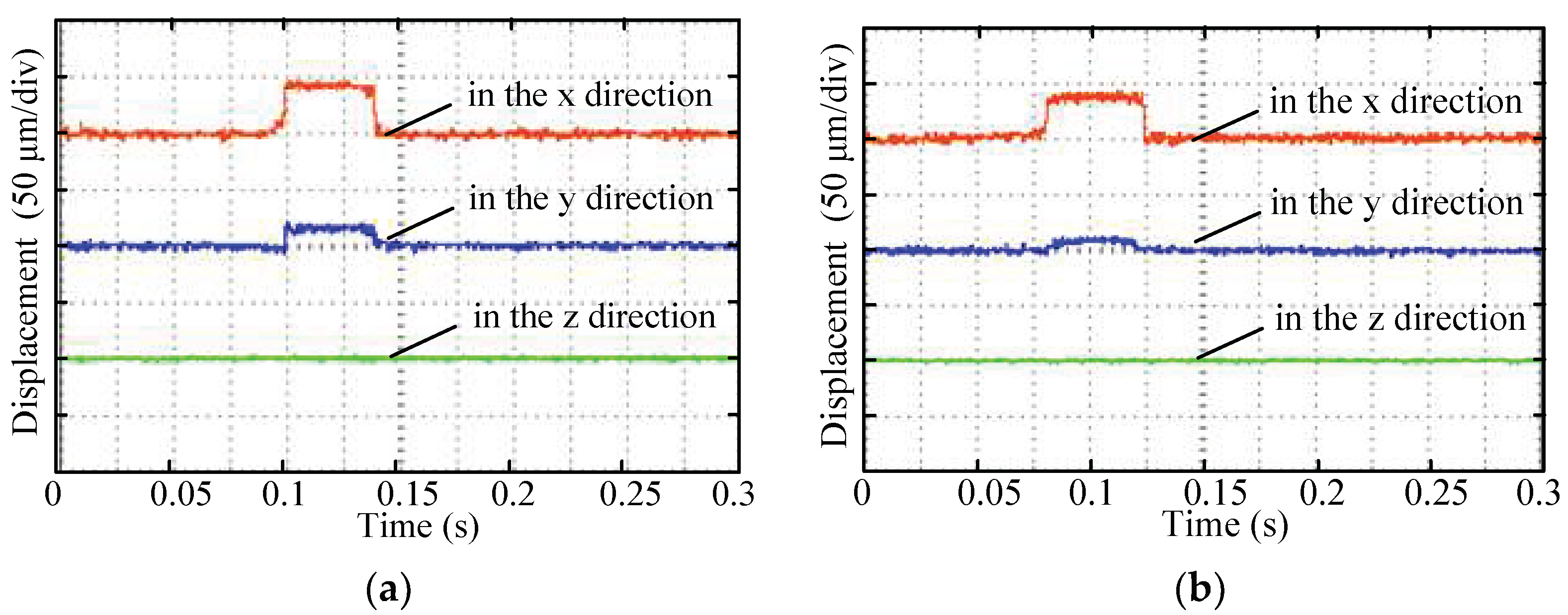
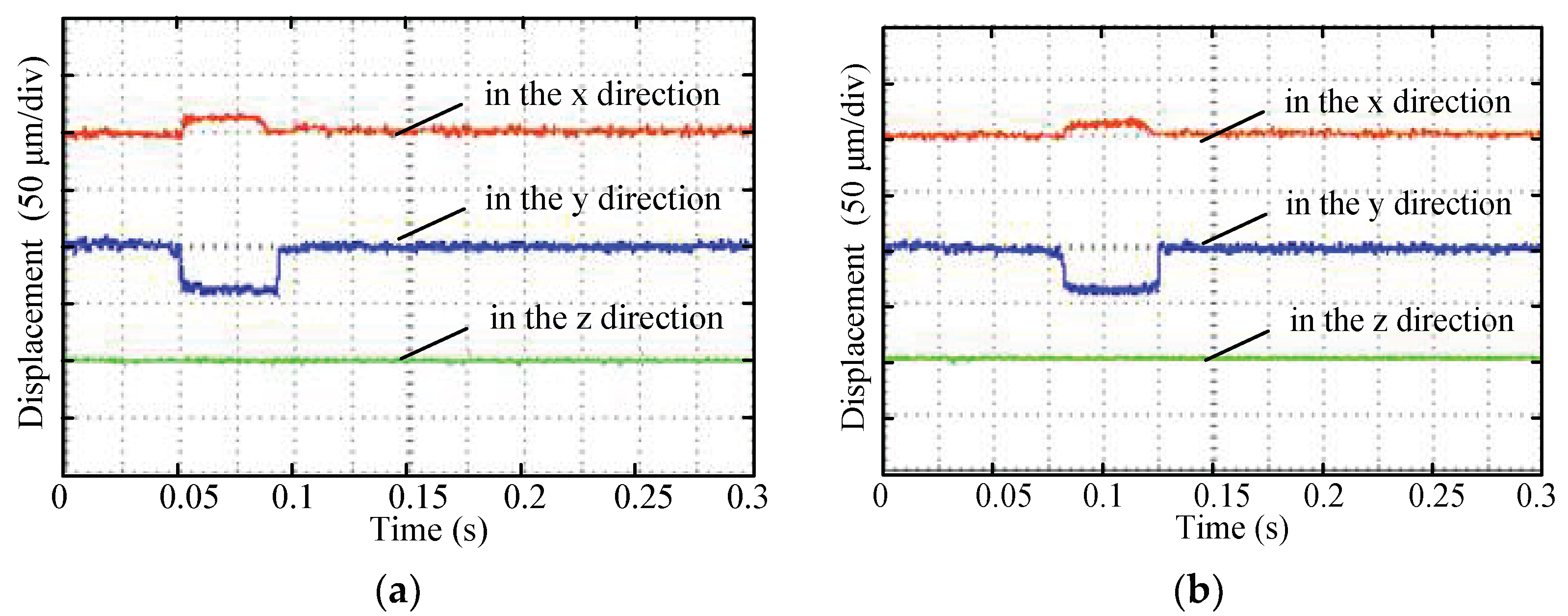
5.3. Coupling Validation Experiment

When the rotor was stable, the external disturbance force was applied with the same weight, 30 N, in the z, x, and y directions, and the response waveforms were as shown in Figure 20, Figure 21 and Figure 22. As shown in Figure 20, the external disturbance force in the axial direction had nearly no influence on the radial direction, and as seen in Figure 21 and Figure 22, the external disturbance force in the radial direction had nearly no influence on the axial direction, which means that there is nearly no coupling between the axial and radial directions. As seen in Figure 21 and Figure 22, when one degree of freedom in the radial direction was disturbed, the displacement of the three-pole RAHMB on the other degree of freedom was larger than the displacement of the six-pole RAHMB, which means that the couplings between the radial variables of the three-pole RAHMB are bigger than the couplings between the radial variables of the six-pole RAHMB.

6. Conclusions

In order to decrease the strong nonlinearity and couplings among the suspension forces with the control currents and displacements which are caused by the asymmetric distribution of the three magnetic poles along the y axis, the six-pole RAHMB is proposed. In order to obtain the radial capacity, the maximum suspension forces of the three-pole and six-pole RAHMBs in each direction were theoretically analyzed. Simulation and experiment results verify that the nonlinearity and couplings of the six-pole RAHMB are all smaller than the nonlinearity and couplings of the three-pole RAHMB. Among them, compared with the radial capacity of 74.6 N of the three-pole RAHMB obtained by simulation, the radial capacity of 83.6 N of the six-pole RAHMB is 12.0% greater. Compared with the radial capacity of 84.1 N of the three-pole RAHMB obtained by experiment, the radial capacity of 94.8 N of the six-pole RAHMB is 12.7% greater. The simulation results are consistent with the experimental results, indicating the correctness of the theoretical analysis.

References

1. Han, X.; Liu, G.; Le, Y.; Dong, B.; Zheng, S. Unbalanced Magnetic Pull Disturbance Compensation of Magnetic Bearing Systems in MSCCs. IEEE Trans. Ind. Electron. 2023, 70, 4088–4097. [Google Scholar] [CrossRef]
2. Le, Y.; Wang, D.; Zheng, S. Design and Optimization of a Radial Magnetic Bearing Considering Unbalanced Magnetic Pull Effects for Magnetically Suspended Compressor. IEEE/ASME Trans. Mechatron. 2022, 27, 5760–5770. [Google Scholar] [CrossRef]
3. Wang, C.; Le, Y.; Zheng, S.; Han, B.; Dong, B.; Chen, Q. Suppression of Gyroscopic Torque Disturbance in High Speed Magnetically Levitated Rigid Rotor Systems Based on Extended State Observer. IEEE/ASME Trans. Mechatron. 2022, 1–11. [Google Scholar] [CrossRef]
4. Hu, H.; Liu, K.; Wang, H.; Wei, J.A. Wide Bandwidth GaN Switching Power Amplifier of Active Magnetic Bearing for a Flywheel Energy Storage System. IEEE Tran. Power Electron. 2023, 38, 2589–2605. [Google Scholar] [CrossRef]
5. Zhang, W.; Wang, J.; Zhu, P.; Yu, J. A Novel Vehicle-Mounted Magnetic Suspension Flywheel Battery With a Virtual Inertia Spindle. IEEE Trans. Ind. Electron. 2022, 69, 5973–5983. [Google Scholar] [CrossRef]
6. Zhang, W.; Yang, H.; Cheng, L.; Zhu, H. Modeling Based on Exact Segmentation of Magnetic Field for a Centripetal Force Type-Magnetic Bearing. IEEE Trans. Ind. Electron. 2020, 67, 7691–7701. [Google Scholar] [CrossRef]
7. Liu, X.; Ma, X.; Feng, R.; Chen, Y.; Shi, Y.; Zheng, S. Model Reference Adaptive Compensation and Robust Controller for Magnetic Bearing Systems With Strong Persistent Disturbances. IEEE Trans. Ind. Electron. 2022, 1–10. [Google Scholar] [CrossRef]
8. Li, J.; Liu, G.; Zheng, S.; Cui, P.; Chen, Q. Micro-Jitter Control of Magnetically Suspended Control Moment Gyro Using Adaptive LMS Algorithm. IEEE/ASME Trans. Mechatron. 2022, 27, 327–335. [Google Scholar] [CrossRef]
9. Han, B.; Chen, Y.; Zheng, S.; Li, M.; Xie, J. Whirl Mode Suppression for AMB-Rotor Systems in Control Moment Gyros Considering Significant Gyroscopic Effects. IEEE Trans. Ind. Electron. 2021, 68, 4249–4258. [Google Scholar] [CrossRef]
10. Sun, M.; Xu, Y.; Chen, S. Research on Electromagnetic System of Large Capacity Energy Storage Flywheel. IEEE Trans. Magn. 2023, 1. [Google Scholar] [CrossRef]
11. Zhu, H.; Wang, S. Decoupling Control Based on Linear/Non-Linear Active Disturbance Rejection Switching for Three-Degree-of-Freedom Six-Pole Active Magnetic Bearing. IET Electr. Power App. 2020, 14, 1818–1827. [Google Scholar] [CrossRef]
12. Wu, M.; Zhu, H. Backstepping Control of Three-Pole Radial Hybrid Magnetic Bearing. IET Electr. Power App. 2020, 14, 1480–1487. [Google Scholar] [CrossRef]
13. Yu, C.; Deng, Z.Q.; Mei, L.; Peng, C.; Cao, X.; Chen, S.; Ding, Q. Evaluation Criteria of Material Selection on 3-DOF Hybrid Magnetic Bearing. IEEE Tran. Ind. App. 2021, 57, 4733–4744. [Google Scholar] [CrossRef]
14. Hemenway, R.; Gjemdal, H.; Severson, L. New Three-Pole Combined Radial–Axial Magnetic Bearing for Industrial Bearingless Motor Systems. IEEE Tran. Ind. App. 2021, 57, 6754–6764. [Google Scholar] [CrossRef]
15. Wang, Z.; Zhang, T.; Wu, S. Suspension Force Analysis of Four-Pole Hybrid Magnetic Bearing with Large Radial Bearing Capacity. IEEE Trans. Magn. 2020, 56, 1–4. [Google Scholar] [CrossRef]
16. Schmidt, E.; Hofer, M. Static and Transient Voltage Driven Finite Element Analysis for the Sensorless Control of a Hybrid Radial Active Magnetic Bearing. In Proceedings of the 2009 International Conference on Electrical Machines and Systems, Tokyo, Japan, 15–18 November 2009; pp. 1–5. [Google Scholar] [CrossRef]
17. Matsuda, K.; Kanemitsu, Y.; Kijimoto, S. Optimal Number of Stator Poles for Compact Active Radial Magnetic Bearings. IEEE Trans. Magn. 2007, 43, 3420–3427. [Google Scholar] [CrossRef]
18. Chen, S.; Hsu, C. Optimal Design of a Three-Pole Active Magnetic Bearing. IEEE Trans. Magn. 2002, 38, 3458–3466. [Google Scholar] [CrossRef]
19. Zhang, W.; Zhu, H.; Yang, Z.; Sun, X.; Yuan, Y. Nonlinear Model Analysis and “Switching Model” of AC–DC Three-Degree-of-Freedom Hybrid Magnetic Bearing. IEEE ASME Trans. Mechatron. 2016, 21, 1102–1115. [Google Scholar] [CrossRef]
20. Zhang, W.; Zhu, H. Control System Design for a Five-Degree-of-Freedom Electrospindle Supported with AC Hybrid Magnetic Bearings. IEEE ASME Trans. Mechatron. 2015, 20, 2525–2537. [Google Scholar] [CrossRef]
21. Chen, S. Nonlinear Smooth Feedback Control of a Three-Pole Active Magnetic Bearing System. IEEE Trans. Control Syst. Technol. 2011, 19, 615–621. [Google Scholar] [CrossRef]
22. Darbandi, S.M.; Behzad, M.; Salarieh, H.; Mehdigholi, H. Linear Output Feedback Control of a Three-Pole Magnetic Bearing. IEEE/ASME Trans. Mechatron. 2014, 19, 1323–1330. [Google Scholar] [CrossRef]
23. Han, B.; Zheng, S.; Le, Y.; Xu, S. Modeling and Analysis of Coupling Performance Between Passive Magnetic Bearing and Hybrid Magnetic Radial Bearing for Magnetically Suspended Flywheel. IEEE Trans. Magn. 2013, 49, 5356–5370. [Google Scholar] [CrossRef]
24. Zhong, Y.; Wu, L.; Huang, X.; Fang, Y.; Zhang, J. An Improved Magnetic Circuit Model of a 3-DOF Magnetic Bearing Considering Leakage and Cross-Coupling Effects. IEEE Trans. Magn. 2017, 53, 1–6. [Google Scholar] [CrossRef]
25. Zhu, H.; Liu, T. Rotor Displacement Self-Sensing Modeling of Six-Pole Radial Hybrid Magnetic Bearing Using Improved Particle Swarm Optimization Support Vector Machine. IEEE Trans. Power Electron. 2020, 35, 12296–12306. [Google Scholar] [CrossRef]
26. Zhong, Y.; Fang, L.; Huang, X. Investigation of cross-coupling effect of a 3-DOF magnetic bearing using magnetic circuit method. In Proceedings of the 2017 20th International Conference on Electrical Machines and Systems (ICEMS), Sydney, Australia, 11–14 August 2017. [Google Scholar] [CrossRef]
Figure 1. The structure of this paper.
Electronics 12 01493 g001
Figure 2. Structure of the (a) three-pole and (b) six-pole radial–axial HMB. (1) Axial stator. (2) Permanent magnet. (3) Axial control coils. (4) Radial stator. (5) Radial control coils. (6) Rotor. After removing the outermost axial stator, the structure of the (c) three-pole and (d) six-pole RAHMB. (e) The axial magnetic flux path of the RAHMB.
Electronics 12 01493 g002
Figure 3. Radial magnetic flux path of the radial–axial HMB with (a) three-pole and (b) six-pole structures. A, B, and C represent the three-phase.
Electronics 12 01493 g003
Figure 4. Equivalent magnetic circuits of the (a) three-pole and (b) six-pole radial–axial HMB.
Electronics 12 01493 g004
Figure 5. The waveforms of Fziz and z of the (a) three-pole and (b) six-pole RAHMB.
Electronics 12 01493 g005
Figure 6. The waveforms of Fxix and x of the (a) three-pole and (b) six-pole RAHMB.
Electronics 12 01493 g006
Figure 7. The waveforms of Fyiy and y of the of the (a) three-pole and (b) six-pole RAHMB.
Electronics 12 01493 g007
Figure 8. The waveforms of Fzz and x of the (a) three-pole and (b) six-pole RAHMB.
Electronics 12 01493 g008
Figure 9. The waveforms of Fxz and x of the (a) three-pole and (b) six-pole RAHMB.
Electronics 12 01493 g009
Figure 10. The waveforms of Fziz and ix of the (a) three-pole and (b) six-pole RAHMB.
Electronics 12 01493 g010
Figure 11. The waveforms of Fxiz and ix of the (a) three-pole and (b) six-pole RAHMB.
Electronics 12 01493 g011
Figure 12. The waveforms of Fxx and y of the (a) three-pole and (b) six-pole RAHMB.
Electronics 12 01493 g012
Figure 13. The waveforms of Fyx and y of the (a) three-pole and (b) six-pole RAHMB.
Electronics 12 01493 g013
Figure 14. The waveforms of Fxix and iy of the (a) three-pole and (b) six-pole RAHMB.
Electronics 12 01493 g014
Figure 15. The waveforms of Fyix and iy of the (a) three-pole and (b) six-pole RAHMB.
Electronics 12 01493 g015
Figure 16. The experiment platform of the RAHMBs.
Electronics 12 01493 g016
Figure 17. The waveforms of Fziz of the (a) three-pole and (b) six-pole RAHMB.
Electronics 12 01493 g017
Figure 18. The waveforms of Fxix of the (a) three-pole and (b) six-pole RAHMB.
Electronics 12 01493 g018
Figure 19. The waveforms of Fyiy of the (a) three-pole and (b) six-pole RAHMB.
Electronics 12 01493 g019
Figure 20. The waveforms of the (a) three-pole and (b) six-pole RAHMB when the rotor is disturbed in the z direction.
Electronics 12 01493 g020
Figure 21. The waveforms of the (a) three-pole and (b) six-pole RAHMB when the rotor is disturbed in the x direction.
Electronics 12 01493 g021
Figure 22. The waveforms of the (a) three-pole and (b) six-pole RAHMB when the rotor is disturbed in the y direction.
Electronics 12 01493 g022