Article

A Model of Thermally Activated Molecular Transport: Implementation in a Massive FPGA Cluster

by
Grzegorz Jabłoński
1,*,
Piotr Amrozik
1 and
Krzysztof Hałagan
2
1
Department of Microelectronics and Computer Science, Lodz University of Technology, 93-005 Łódź, Poland
2
Department of Molecular Physics, Lodz University of Technology, 90-924 Łódź, Poland
*
Author to whom correspondence should be addressed.
Electronics 2023, 12(5), 1198; https://doi.org/10.3390/electronics12051198
Submission received: 18 January 2023 / Revised: 8 February 2023 / Accepted: 28 February 2023 / Published: 2 March 2023
(This article belongs to the Special Issue Applications Enabled by FPGA-Based Technology)

Abstract

:
In this paper, a massively parallel implementation of Boltzmann’s thermally activated molecular transport model is presented. This models allows taking into account potential energy barriers in molecular simulations and thus modeling thermally activated diffusion processes in liquids. The model is implemented as an extension to the basic Dynamic Lattice Liquid (DLL) algorithm on ARUZ, a massively parallel FPGA-based simulator located at BioNanoPark Lodz. The advantage of this approach is that it does not use any exponentiation operations, minimizing resource usage and allowing one to perform simulations containing up to 4,608,000 nodes.

1. Introduction

Computer simulations have become one of the most important research methods for non-equilibrium processes in chemistry and physics. The applied simulation techniques, however, have encountered difficulties with different types of problems, related to spatial and time scales, which are necessary to bring the system to a state of full equilibrium. Such phenomena are particularly interesting wherever the enthalpy factor (non-covalent interactions between molecules and atoms) is important (e.g., in soft matter, simple and complex liquids, and polymer solutions), as well as when temperature is one of the parameters of the studied phenomenon. The commonly used computational methods for non-equilibrium problems, such as phase separation, include nonlinear diffusion equation solvers [1,2], molecular dynamics methods [3], and stochastic Monte Carlo (MC) methods [4,5].
A particularly interesting method belonging to the stochastic category is the Dynamic Lattice Liquid (DLL) model [6,7,8], as it allows observing not only steady state static behavior but also the process of reaching equilibrium. It is based on the concept of cooperative motion of objects (elements). The positions of the elements are limited to the nodes of a face-centered cubic (FCC) lattice (coordination number Z = 12) for simplicity. The FCC lattice is commonly chosen in 3D as it has the highest coordination number among regular ones. The algorithm works on a completely occupied lattice, where the elements cannot easily move over a long distance due to the occupation of all neighboring lattice sites. In this case, the only way to move the elements with the excluded volume preserved is cooperative motion. In DLL, cooperative rearrangements take the form of closed loops of displacements that involve at least three elements (see Figure 1). Loops are formed spontaneously in a random way. The DLL model fulfills the continuity equation and provides the correlated movements of molecules as a model of real liquids. A discussion of the detailed balance and ergodicity in the DLL model was presented in [9].
This basic version of the DLL algorithm (also called the LOOPS mechanism here) models Brownian diffusion in a long time limit for simple liquids. However, to model more complex phenomena, the DLL model can be extended with additional functionalities, namely the so-called “mechanisms”:
  • The introduction of molecular bonds with excluded volume between elements must involve the BONDS mechanism, which is responsible for movement restriction related to the length-constant unbreakable bonds.
  • The mechanisms BOND_BINDS and BOND_BREAKS are used when one wants to simulate the macromolecular polymerization and degradation processes, respectively.
  • A growing macromolecule (in the case of polymerization, where new elements are joined to the molecule with some probability) can be terminated randomly using the TERMINATION mechanism.
  • Chemical reactions of different orders can also be modeled with the REACTION mechanism, where elements can change their type with a given probability.
  • Local trapping can be modeled with the MOBILITY mechanism, where movement of a given element can be restricted (e.g., due to its spatial position in the simulation box).
  • Vector fields can be modeled using the VECTOR and REORIENTATION mechanisms.
  • In the case where vacancies are present, the WAYS mechanism is used to model cooperative motion involving empty lattice nodes, forming a cooperative set of elements (chain-like and not necessarily a loop).
  • The APERIODIC mechanism is used to build immobile obstacles such as walls.
  • Thermal noise can be reduced in simulations by lowering the temperature with the ENERGY mechanism (introducing potential energy barriers).
All the above mechanisms can be defined for a given type of element or spatial position in the simulation box, enabling modeling of various external fields.
The DLL model can be implemented efficiently with good scalability on a parallel machine equipped with low-latency communication interfaces to the nearest neighbors. A specialized field-programmable gate array (FPGA)-based simulator—ARUZ—was built for DLL simulations and has achieved performance orders of magnitude better than implementations on a sequential computer (see Table 4 in [10]).
In this paper, the details of Boltzmann’s thermally activated molecular transport model [11] implemented as a DLL extension on ARUZ (ENERGY mechanism) are presented. The model allows taking into account potential energy barriers in molecular simulations and thus allows modeling of thermally activated diffusion processes in liquids. This approach does not use any exponentiation operations, allowing one to perform simulations containing 4,608,000 nodes, reaching 69 percent of the maximum simulation size achievable using only the LOOPS mechanism.
The performed simulations confirm that the implementation gives exact results compared with the values calculated theoretically.
Although the presented implementation works as an extension of the DLL algorithm, it is also applicable to other molecular movement models, especially those based on the lattice approach with high occupancy, such as direct exchange dynamics [12] or vacancy transport [13].

2. The ARUZ Simulator

The ARUZ [10], commissioned at the end of 2015 at Lodz Technopark (currently BioNanoPark), came as a result of close cooperation between the Department of Molecular Physics and the Department of Microelectronics and Computer Science, both from the Lodz University of Technology, complemented by the professional management expertise of the Ericpol (currently Ericsson) company. It is the first instance of a simulator built using TAUR technology [14]. This machine was designed to reflect the DLL algorithm in its hardware [15].
The ARUZ simulator consists of 2880 simulation boards called daughter boards (DBoards), interconnected by ca. 75,000 cables (see Figure 2). Each of them carries nine FPGAs: eight of them being called DSlaves (Artix XC7A200T), which constitute the resources for the nodes of the simulation algorithm, and the remaining one called DMaster (Zynq XC7Z015), which manages the operation of the DSlaves. The entire ARUZ thus contains 23,040 DSlaves. Each of the DSlaves can host up to a few hundred simulation nodes, depending on which features of the computational model are selected, and has communication interfaces to the eight closest neighboring FPGAs in a 3D simulation space.
Internally, each FPGA implements a grid of specialized processing cells dedicated to performing consecutive steps and complex calculations of the Dynamic Lattice Liquid algorithm. Assuming that every FPGA can host ca. 300 DLL cells [10], the entire simulation space consists of about 6.9 million nodes in the case of the basic DLL version.

3. Thermally Activated Diffusion Model

In the DLL algorithm, the individual molecules try to move in random directions, and the movement is possible only if the set of molecules is able to form a cooperative loop, where excluded volume interactions are naturally accounted for. The thermally activated diffusion model introduces an additional temperature-dependent restriction on molecule movement due to their interaction with neighbors. Such simulations have been performed previously only on a sequential computer [16,17,18], and no high-performance parallel implementation of this model is known. Different models can be considered in this case, including the kinetic MC test [16] based on the present state, forward-testing based on the next state, Metropolis sampling [4], or Glauber dynamics [19]. The first one was selected for the sake of simplicity and high performance. Additionally, the rest of the models take into account the forward system configuration, which would require a reversing phase of the simulation (going back to the starting point if the test fails), which complicates the parallel architecture a lot. Only the nearest neighbors were taken into account to simplify the interconnection topology and limit the number of transmission phases, but this simplification is not really significant in dense systems where long-distance interactions are mostly shielded by the rest of the system.
The ENERGY algorithm computes the probability of molecule movement in the following simulation phase (cooperative loops). Based on this probability, a pseudo-random number generator determines if the given molecule is immobilized in the current DLL cycle.
The involvement of nearest-neighbor interactions (or, in other words, temperature-dependent attraction or repulsion) must take into account the probability test related to the system energy. The system Hamiltonian for the ith lattice site populated by the X-type element is defined as follows:
E i k B T = 1 k B T ( 1 2 j ε X Y j + H X i )
where the sum extends over all nearest neighbors and j can take any type Y. The following definitions apply:
  • T is the absolute temperature, and k B is the Boltzmann constant.
  • H X / k B T is the interaction energy of the type X with the external field and can depend on the spatial position to model, for example, the temperature gradient.
  • ε X Y / k B T is the interaction energy of the i , j pair and is position-independent. In the presented model, ε X Y always equals ε Y X .
Both ε X Y / k B T and H X / k B T are input data. For example, if four interactions ε X Y between elements are defined, with X = A placed in the currently analyzed ith lattice node and Y = A , B , C , D , then
E i k B T = 1 2 k B T ( ε A A n A A + ε A B n A B + + ε A C n A C + ε A D n A D ) + H A i k B T
with multiplicities of i , j pairs n A A = 2 , n A B = 2 , n A C = 1 , and n A D = 1 , as illustrated in Figure 3.
A kinetic Monte Carlo test, representing the Boltzmann statistics, is applied (i.e., an effective attempt of motion is performed with a probability proportional to the energy of the current local state) [16,20]:
P i = e E i k B T
The test is executed for all elements in a given loop of possible cooperative movement, and all elements must pass it; otherwise, the whole loop is immobilized (when e x p ( E i / k B T ) < r a n d o m [ 0 , 1 ) ).
As a result, if ε X Y > 0 , then an attractive interaction is present for the i , j pair. Interactions become effective at a finite temperature by reducing the probability of motion. Here, ε X Y  describes the barrier which has to be overcome in order to release contact between X and Y during the thermally activated diffusion process.
The average interaction energy per element is equal to < E > = 1 / N i = 1 N E i , with N being the total number of elements in the lattice.
Note that the commonly known Metropolis sampling algorithm is not used because the loops have a spatial extent (over large distances, sometimes even 50 lattice constants [10]), and the test defined above involves the nearest neighbors only [21].

4. Implementation Requirements

To implement the kinetic MC test, the types of all the neighbors must be known. These are obtained using the local communication, described in detail in [10] (see Figure 11 therein for details about latency). After this information is acquired, the computations are performed independently in all nodes. The DLL algorithm’s performance is mainly determined by the performance of the loop detection phase [22]. The time of a single cycle of the LOOPS algorithm amounts to ca. 100 microseconds. Therefore, in implementation of the ENERGY mechanism, the minimization of resource utilization and not the lowest latency is the main objective.
Implementing the test in a digital circuit requires choosing the number storage format and the required precision. Equation (3) contains the exponentiation, which is a quite complex operation that is difficult to implement in hardware.
By substituting (1) into (3), we obtain
P i = e ( 1 2 k = 1 Z ε X Y k B T ( k ) + H X ( x , y , z ) )
where Z is the number of neighbors, which is assumed to be 12. If we define
ε w ( X , Y ) = e ( 1 2 ε X Y k B T ) and ε e ( X ) = e ( H X ( x , y , z ) )
then we obtain
P i = k = 1 Z ε w ( X , Y k ) · ε e ( X )
As ε w ( X , Y k ) and ε e ( X ) are constant, no exponentiation operation is needed in the FPGA fabric, as they can be precomputed in the software.
For
y = e x
we have
d y = e x d x
Thus, we have
d y y = e x y d x
and
d y y = d x
Therefore, the absolute precision of x is equal to the relative precision of y. Therefore, to store ε w and ε e and perform operations on them, we need to apply a floating-point format, as it ensures a constant relative precision for the full range of stored values.
Because the assumed precision of the expression in the exponent in Equation (4) is 10 5 , and l o g 2 ( 10 5 ) is −16.7, to store ε w and ε e , we need a 17 bit mantissa.
Assuming that 1 2 ε X Y k B T ( k ) in H X ( x , y , z ) has a range −10–10, from Equation (4), we can infer that P i can vary in the range e 10 · ( Z + 1 ) e 10 · ( Z + 1 ) , which is thus e 10 · 13 e 10 · 13 , 2 187.55 2 187.55 , and 2 2 7.55 2 2 7.55 . This implies 9 bits for the floating point number exponent (8 for numbers greater than 1 and 8 for numbers smaller than 1) to encompass the entire range presented above.
In the vast majority of cases, the maximum number of simulation time steps is assumed to be 10 9 . The mean probability of element movement is close to 6% for the FCC lattice [23] in the case of a basic version of DLL (additional mechanisms can only decrease it). Therefore, the number of steps in which the energy test will be used is approximately 0.06 × 10 9 = 6 × 10 7 per element, so it will be necessary to perform the operation with probabilities in the order of 1 / ( 6 × 10 7 ) . L o g 2 ( 6 × 10 7 ) = 25.8 , and therefore we need at least a 26 bit pseudo-random number generator. Please note that we do not need to compute a logarithm of the pseudo-random number as opposed to, for example, the solution presented in [24].

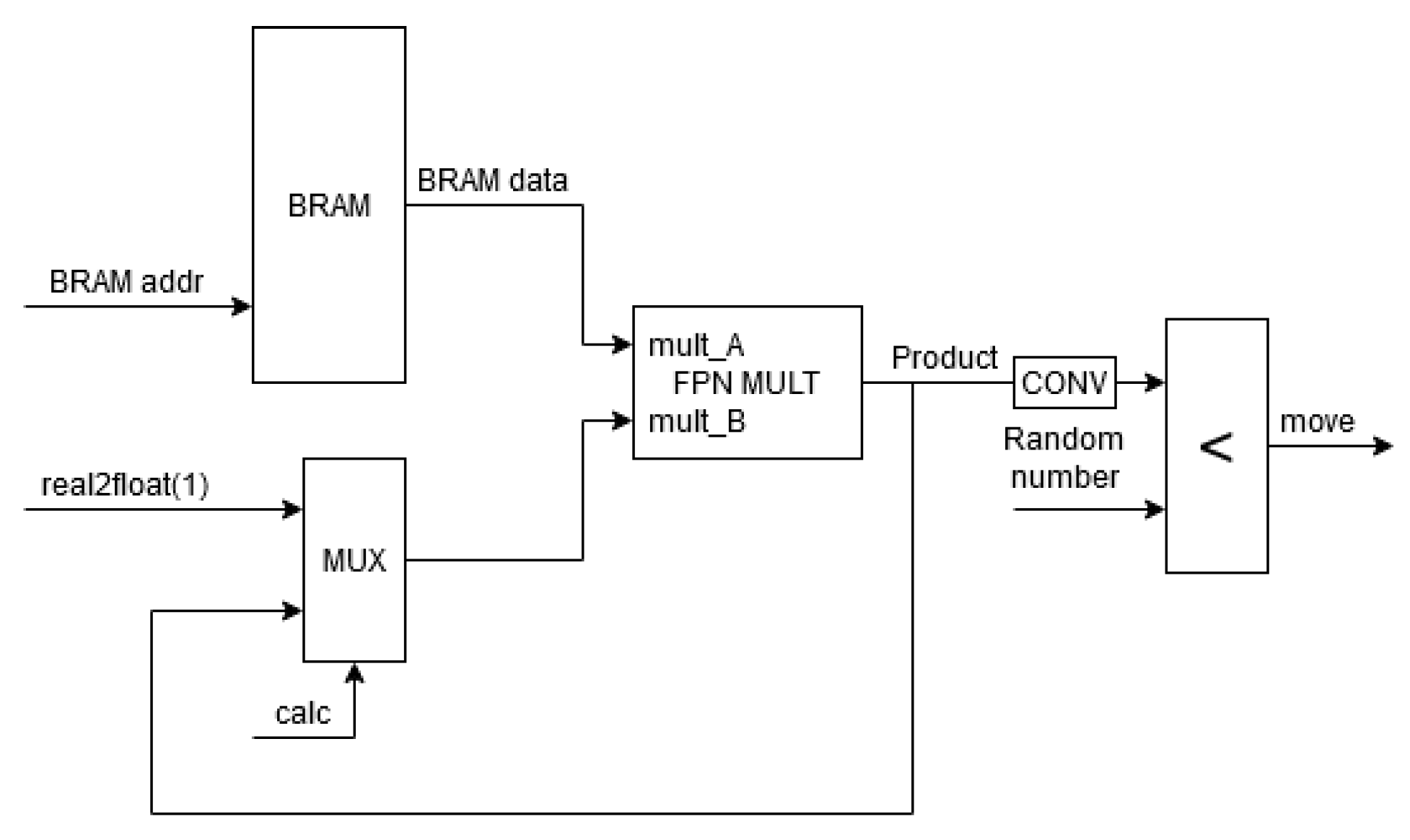
5. Implementation on FPGA

As the number of simulation nodes in DSlave (Artix XC7A200T) is limited to ca. 300, the optimization of the amount of hardware resources used by each node becomes a crucial factor. As can be seen in Figure 16 in [10], the most limiting resources are look-up tables (LUTs). Therefore, implementation using other available FPGA resources is desirable. The kinetic Monte Carlo test requires Z + 1 multiplications of ε w and ε e , as presented in Equation (6). This can be performed effectively by employing specialized hardware resources available in DSlave instead of configurable logic blocks (CLBs) [25], such as block random access memory (BRAM) [26] to store coefficients ε w and ε e and digital signal processing (DSP) slices [27] to perform multiplications.
Artix XC7A200T has 13,140 kb of BRAM [28] and 740 DSP slices, each containing a 25 × 18 multiplier. To implement multiplications in Equation (6), a single Xilinx Floating-Point Operator IP core [29] was used. This multiplier needs two DSP slices, limiting the number of nodes that can be implemented in one DSlave to 370. The block diagram of a module implementing the kinetic Monte Carlo test is presented in Figure 4.
To reduce the number of CLBs, a special method for addressing BRAM is used which allows the concatenation of address vectors instead of employing more complicated calculations. The memory address is a concatenation of the following (see Table 1):
  • An “e_offset” bit indicating parts of the memory storing ε w and ε e ;
  • A vector representing the type of a neighbor element “other_type”;
  • A vector representing the type of the considered element “my_type” (occupying the right-most bits).
The coefficient memory is divided into two sections. The first section of the memory stores ε w coefficients and requires M 2 memory locations (assuming that ε w occupies one location), where M is the number of types rounded up to the nearest power of two. The second section of the memory stores ε e coefficients and requires M memory locations (assuming that ε e occupies one location). Therefore, the total number of memory locations is M 2 + M .
In Table 1 an example of memory addressing is presented:
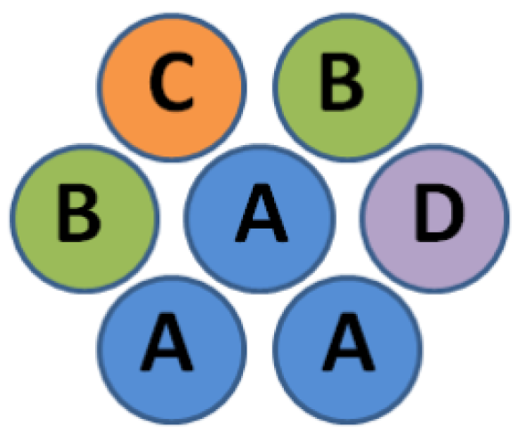
  • Example 1: Four element types are used (types A, B, C, and D coded by a two-bit vector: A = 00, B = 01, C = 10, and D = 11). The address of an appropriate ε w is a concatenation of the ”e_offset” bit set to 0, and two two-bit vectors (representing the type of the considered element and a neighbor, respectively). The address of ε e is the concatenation of a constant M 2 coded by a three-bit vector (taking bits of ”e_offset” and ”other_type” vectors) and a two-bit vector representing the type of element considered. In this example, all memory locations are used, and 16 of them are needed for ε w and 4 for ε e , leading to a total of 20.
  • Example 2: Three element types are used (types A, B, and C coded by a two-bit vector: A = 00, B = 01, and C = 10). The addresses of the appropriate coefficients ε w and ε e are determined in the same way as in the previous example. Only gray-colored memory locations are used, but the required number of memory locations is still 20.
As the presented example shows, some parts of the memory are unused in some scenarios, and the memory utilization is higher than would be expected based on the number of types, but calculation of the memory address is kept very simple, and its implementation costs less CLBs for one node.
The FPN MULT block (see Figure 4) is 27 × 27 (1 bit for the sign, 10 bits for the exponent, and 16 bits for the mantissa) floating-point multiplier. The BRAM data are fed to the mult_A input of the multiplier. The data on the mult_B input are multiplexed. During the first cycle of calculations, the value of one represented in the floating-point format, and during the following cycles, the current product is fed. In this way, the result accumulates, giving Equation (6) after Z + 1 = 13 multiplication cycles.
Figure 5 presents the results of an example simulation that shows the module’s operation. Its settings are as follows: a single type A surrounded by a homogeneous mixture of types B and C, ε A B / k B T = 0.2 , and ε A C / k B T = 0.01 . Thus, e ( 1 2 · k = 1 Z 2 0.2 1 2 · k = 1 Z 2 0.01 ) = k = 1 Z 2 e ( 1 2 · 0.2 ) · k = 1 Z 2 e ( 1 2 · 0.01 ) = k = 1 Z 2 0.90483 · k = 1 Z 2 0.99501 = 0.53255
In this simulation, one floating-point multiplication takes 4 clock cycles, so the whole operation takes 12 · 4 = 48 clock cycles. The clock period is 8 ns.
In the example, the neighbor nodes are placed evenly (homogeneous mixture). Thus, the BRAM address takes two values: four (0100), where ε w ( B , A ) is stored, and eight (1000), where ε w ( C , A ) is stored. The values read from BRAM are 0.90483 and 0.99501 , respectively. The result is 0.5325469 , which is correct.
The output of “FPN MULT” is compared with a random number. This random number is a 32 bit vector generated by a dedicated linear feedback shift register (LSFR). To make this comparison possible, the product is converted to a 32 bit fixed-point number. Both numbers being compared are treated as numbers in the range [ 0 , 1 ) . The flag “move” is set to one when the “product” is greater than the generated random number.
There are two parameters of the floating-point multiplier core affecting the resource utilization and timing closure that can be adjusted: latency and DSP usage. Latency can be configured to between 0 and 8 clock cycles. The multiplier can use zero (“no DSP”), one (“full DSP” setting), or two (“max DSP”) DSP48 blocks per instance.
Table 2 summarizes the results of exploration of a design space and shows the overhead of adding the ENERGY mechanism to the simulation. The results for the maximum number of nodes that can be placed in a single FPGA that can be successfully implemented without timing issues are presented in the table.
The maximum number of simulation nodes that can be placed in a DSlave is limited by the number of LUTs. It is typically not possible to route a design with more than 80% LUT utilization. Increasing the latency of the multiplier improves the timing closure but also slightly increases resource utilization. The timing closure is not possible with the multiplier latency set to one. Setting it to two results in successful implementation only for three out of all eight DSlaves on the board. It is possible to obtain consistently positive results for the synthesis with the latency set to at least three. At the “max DSP” setting, over half of the DSPs are used. As the only other mechanism that is able to use DSPs is the WAYS mechanism [22], and it uses only one DSP48 block per node, this is not a limiting factor. However, halving DSP usage by applying the “full DSP” setting does not cause a significant increase in LUTs. On the other hand, using the “no DSP” setting increases the LUT usage, enormously reducing the maximum number of nodes per chip to 128.
The inclusion of the ENERGY mechanism consumes ca. 20% of the LUTs in fully utilized FPGA. As a result, it decreases the maximum number of nodes per chip to 200 (4,608,000 in the entire machine) compared with 288 for the simulation using only LOOPS.

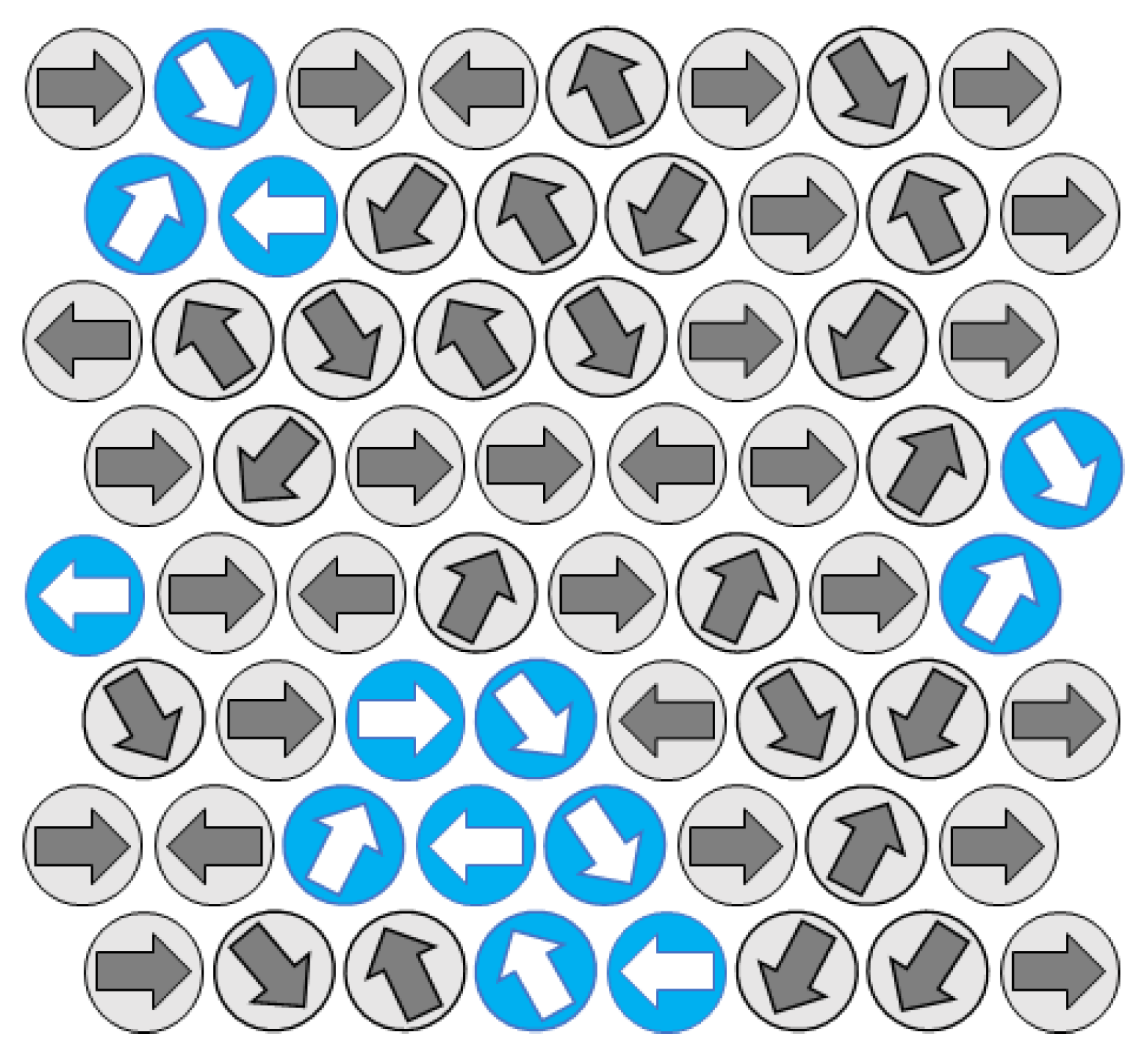
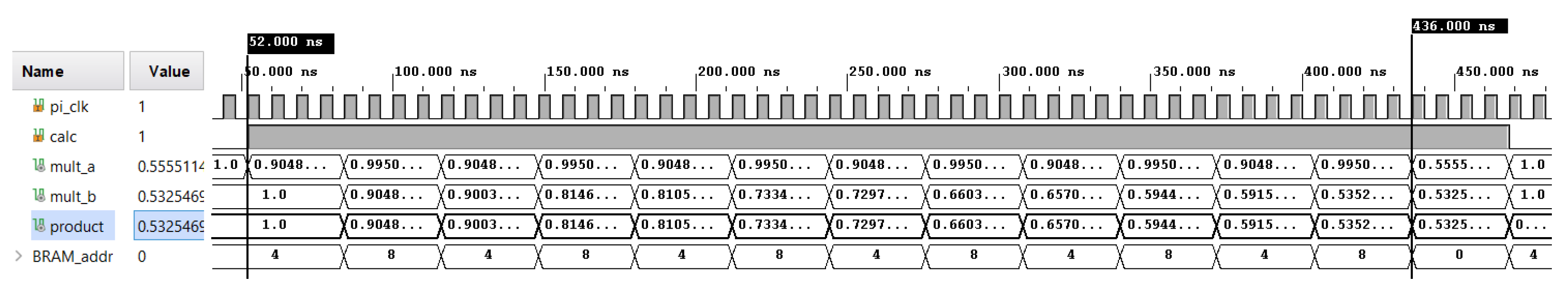
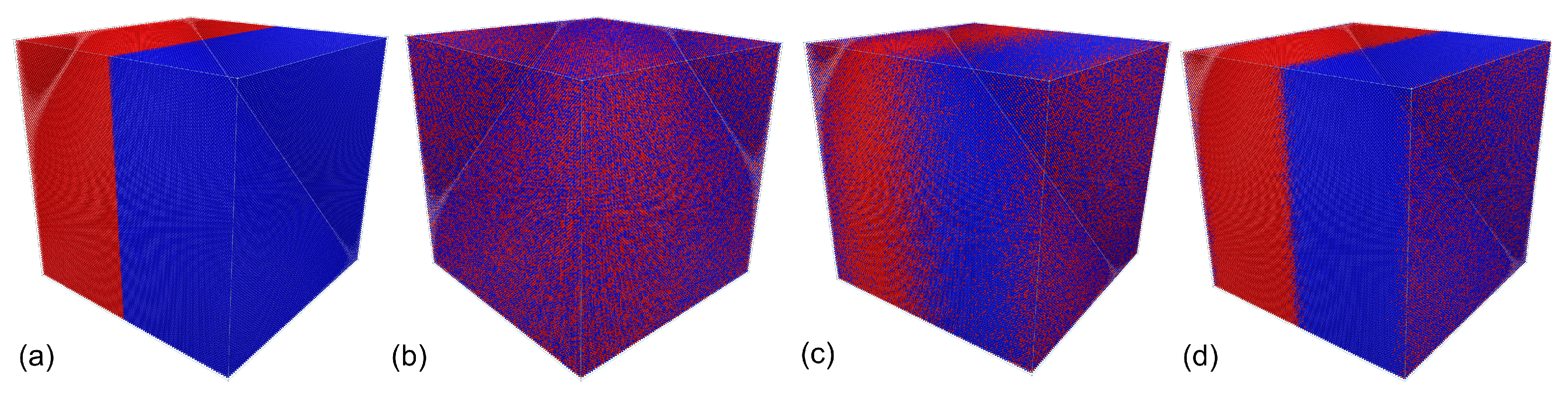
6. Example Simulation

The Hamiltonian in Equation (1) can model a kind of system called the conserved-order parameter [30] Ising model [31], or model B in the Hohenberg–Halperin classification [32]. The model assumes that the diffusion can be suppressed in X(Y)-type-rich regions ( ε X X ( Y Y ) / k B T > 0 ) or at the X-Y interfaces [33] ( ε X Y / k B T > 0 ) as a result of nearest-neighbor interactions.
As the probability of any state in equilibrium is given by the Boltzmann distribution, the interaction ε X Y causes configurations where particles are clustered together to be low in energy and therefore more likely at low temperatures. The critical interaction value for the FCC lattice (defined with a critical temperature T C ) after which the systems undergo the order-disorder transition (second-order phase transition) is ε / 2 k B T C = 0.204...[34,35].
This kind of system was used to study many physical problems for which the kinetics of mixing or demixing matters (i.e., where diffusivity of elements is highly related to their neighborhood), such as for binary alloys [36,37], liquid mixtures [38,39], and polymer blends [40,41]. Obviously, if more than two types with many more pairs of interactions are defined, then the modeled system possesses much higher complexity than the simple Ising model, and its properties strictly depend on the defined conditions.
Figure 6 presents simulation snapshots for a box initially filled with two interacting types: X = A and Y = B (50%:50%). The system consisted of 3,538,944 nodes with periodic boundary conditions. In the first simulation step, the types were fully separated (see Figure 6a in all cases). Figure 6b presents the box configuration after t = 10 5 cycles of the algorithm and ε A B / 2 k B T = 0 (no interaction). The box was mixed by diffusive motion of the elements (by the LOOPS mechanism [10,22]), ending with the totally random configuration. When the interaction was set to ε A B / 2 k B T = 0.1 (Figure 6c), the mixing process was slowed because diffusive motion was limited in the areas where A and B were in contact. However, after t = 10 6 , in this case, the system was again random. The application of ε A B / 2 k B T = 0.5 (Figure 6d) resulted in a stable separation in time because the critical value of the interaction for the FCC lattice was exceeded, and the system remained ordered. The introduction of ε A B / 2 k B T does not restrict movement within regions rich in A or B ( ε A A / 2 k B T and ε B B / 2 k B T were set to zero). In the investigated cases, ARUZ achieved a performance of 5260 cycles/s ( 18.6 × 10 9 lattice updates per second (LUPS) [10]) for ε A B / 2 k B T = 0.01 and up to 7300 cycles/s ( 25.8 × 10 9 LUPS) for ε A B / 2 k B T = 0.1 with a completely random initial configuration because the energy tests excluded 4 6 % of all elements from the diffusive motion analysis in this case.

7. Conclusions

An efficient approach to FPGA-based simulation of Boltzmann’s thermally activated diffusion was developed. It avoids the expensive exponentiation operation in the FPGA fabric by using precomputed values of the Boltzmann weights. A special method for BRAM addressing was used, eliminating complicated calculations thanks to address vector concatenation. Application of the described model increased the performance of the simulation measured in LUPS, as the energy tests excluded a large portion of all elements from diffusive motion. The simulations performed confirmed that the implementation gives exact results compared with the theoretically calculated values.
The presented implementation is applicable to other lattice algorithms where Boltzmann weights need to be used.

Author Contributions

Conceptualization, K.H.; methodology, G.J., P.A. and K.H.; software, G.J. and P.A.; validation, P.A. and K.H.; formal analysis, G.J.; investigation, G.J., P.A. and K.H.; data curation, K.H.; writing—original draft preparation, G.J.; writing—review and editing, G.J., P.A. and K.H.; visualization, K.H.; supervision, G.J. All authors have read and agreed to the published version of the manuscript.

Funding

This research was funded by Polish National Science Centre grant UMO-2017/25/B/ST5/01110.

Data Availability Statement

Not avaliable.

Conflicts of Interest

The authors declare no conflict of interest.

Abbreviations

The following abbreviations are used in this manuscript:
ARUZAnalyzer of Real Complex Systems
(in Polish: Analizator Rzeczywistych Układów Złożonych)
BRAMBlock random access memory
DLLDynamic Lattice Liquid
FCCFace-centered cubic
FPGAField-programmable gate array
LUPSLatice updates per second
TAURTechnology of Real Word Analyzers
(in Polish: Technologia Analizatorów Układów Rzeczywistych)

References

  1. Cahn, J.W.; Hilliard, J.E. Free energy of a nonuniform system. I. Interfacial free energy. J. Chem. Phys. 1958, 28, 258–267. [Google Scholar] [CrossRef]
  2. Cahn, J.W. On Spinodal Decomposition. Acta Metall. 1961, 9, 795–801. [Google Scholar] [CrossRef]
  3. Binder, K.; Ciccotti, G. Monte Carlo and Molecular Dynamics of Condensed Matter; Società Italiana di Fisica: Bologna, Italy, 1996. [Google Scholar]
  4. Metropolis, N.; Rosenbluth, A.W.; Rosenbluth, M.N.; Teller, A.H.; Teller, E. Equations of State Calculations by Fast Computing Machines. J. Chem. Phys. 1953, 21, 1087–1092. [Google Scholar] [CrossRef] [Green Version]
  5. Binder, K.; Heerman, D.W. Monte Carlo Simulation in Statistical Physics. An Introduction, 4th ed.; Springer: Berlin, Germany, 2002. [Google Scholar]
  6. Pakuła, T.; Teichmann, J. Model for Relaxation in Supercooled Liquids and Polymer Melts; MRS Online Proceedings Library: Berlin/Heidelberg, Germany, 1996; Volume 455, p. 211. [Google Scholar] [CrossRef]
  7. Polanowski, P.; Jeszka, J.K.; Matyjaszewski, K. Polymer brushes in pores by ATRP: Monte Carlo simulations. Polymer 2020, 211, 123124. [Google Scholar] [CrossRef]
  8. Kozanecki, M.; Halagan, K.; Saramak, J.; Matyjaszewski, K. Diffusive properties of solvent molecules in the neighborhood of a polymer chain as seen by Monte-Carlo simulations. Soft Matter 2016, 12, 5519–5528. [Google Scholar] [CrossRef] [Green Version]
  9. Pakula, T. Simulation on the completely occupied lattices. In Simulation Methods for Polymers; Marcel Dekker: New York, NY, USA; Basel, Switzerland, 2004. [Google Scholar]
  10. Kiełbik, R.; Hałagan, K.; Zatorski, W.; Jung, J.; Ulański, J.; Napieralski, A.; Rudnicki, K.; Amrozik, P.; Jabłoński, G.; Stożek, D.; et al. ARUZ—Large-scale, massively parallel FPGA-based analyzer of real complex systems. Comput. Phys. Commun. 2018, 232, 22–34. [Google Scholar] [CrossRef]
  11. Jabłoński, G.; Amrozik, P.; Hałagan, K. Molecular Simulations Using Boltzmann’s Thermally Activated Diffusion—Implementation on ARUZ—Massively-parallel FPGA-based Machine. In Proceedings of the 2021 28th International Conference on Mixed Design of Integrated Circuits and System, Lodz, Poland, 24–26 June 2021; pp. 128–131. [Google Scholar] [CrossRef]
  12. Kawasaki, K.; Ohta, T. Theory of Early Stage Spinodal Decomposition in Fluids near the Critical Point. II. Prog. Theor. Phys. 1978, 59, 362–374. [Google Scholar] [CrossRef] [Green Version]
  13. Yaldram, K.; Binder, K. Spinodal decomposition of a two-dimensional model alloy with mobile vacancies. Acta Metall. Mater. 1991, 39, 707–717. [Google Scholar] [CrossRef]
  14. Jung, J.; Kiełbik, R.; Hałagan, K.; Polanowski, P.; Sikorski, A. Technology of Real-World Analyzers (TAUR) and its practical application. Comput. Methods Sci. Technol. 2020, 26, 69–75. [Google Scholar]
  15. Polanowski, P.; Jung, J.; Kielbik, R. Special Purpose Parallel Computer for Modelling Supramolecular Systems based on the Dynamic Lattice Liquid Model. Comput. Methods Sci. Technol. 2010, 16, 147–153. [Google Scholar] [CrossRef]
  16. Pakula, T.; Cervinka, L. Modeling of medium-range order in glasses. J. Non-Cryst. Solids 1998, 232–234, 619–626. [Google Scholar] [CrossRef]
  17. Halagan, K.; Polanowski, P. Kinetics of spinodal decomposition in the Ising model with Dynamic Lattice Liquid (DLL) dynamics. J. Non-Cryst. Solids 2009, 355, 1318–1324. [Google Scholar] [CrossRef]
  18. Halagan, K.; Polanowski, P. Order-disorder transition in 2D conserved spin system with cooperative dynamics. J. Non-Cryst. Solids 2015, 127, 585–587. [Google Scholar] [CrossRef]
  19. Glauber, R.J. Time-Dependent Statistics of the Ising Model. J. Math. Phys. 1963, 4, 294–307. [Google Scholar] [CrossRef]
  20. Pakula, T. Collective dynamics in simple supercooled and polymer liquids. J. Mol. Liq. 2000, 86, 109–121. [Google Scholar] [CrossRef]
  21. Hałagan, K. Investigation of Phase Separation and Spinodal Decomposition Phenomena with Cooperative Dynamics. Ph.D. Thesis, Lodz University of Technology, Łódź, Poland, 2013. [Google Scholar]
  22. Kiełbik, R.; Hałagan, K.; Rudnicki, K.; Jabłoński, G.; Polanowski, P.; Jung, J. Simulation of diffusion in dense molecular systems on ARUZ—Massively-parallel FPGA-based machine. Comput. Phys. Commun. 2023, 283, 108591. [Google Scholar] [CrossRef]
  23. Polanowski, P.; Pakula, T. Studies of mobility, interdiffusion, and self-diffusion in two-component mixtures using the dynamic lattice liquid model. J. Chem. Phys. 2003, 118, 11139–11146. [Google Scholar] [CrossRef]
  24. Migacz, S.; Dutka, K.; Gumienny, P.; Marchwiany, M.; Gront, D.; Rudnicki, W.R. Parallel Implementation of a Sequential Markov Chain in Monte Carlo Simulations of Physical Systems with Pairwise Interactions. J. Chem. Theory Comput. 2019, 15, 2797–2806. [Google Scholar] [CrossRef]
  25. 7 Series FPGAs Configurable Logic Block. Available online: https://docs.xilinx.com/v/u/en-US/ug474_7Series_CLB (accessed on 17 January 2023).
  26. 7 Series FPGA Memory Resources User Guide. Available online: https://docs.xilinx.com/v/u/en-US/ug473_7Series_Memory_Resources (accessed on 17 January 2023).
  27. 7 Series DSP48E1 Slice User Guide. Available online: https://docs.xilinx.com/v/u/en-US/ug479_7Series_DSP48E1 (accessed on 17 January 2023).
  28. 7 Series Product Selection Guide. Available online: https://www.xilinx.com/content/dam/xilinx/support/documents/selection-guides/7-series-product-selection-guide.pdf (accessed on 17 January 2023).
  29. Floating–Point Operator v7.1 LogiCore IP Product Guide. Available online: https://www.xilinx.com/content/dam/xilinx/support/documents/ip_documentation/floating_point/v7_1/pg060-floating-point.pdf (accessed on 17 January 2023).
  30. Newman, M.E.J.; Barkema, G.T. Monte Carlo Methods in Statistical Physics; Clarendon Press: Oxford, UK, 1999. [Google Scholar]
  31. Ising, E. Beitrag zur Theorie des Ferromagnetismus. Z. Physik 1924, 31, 253. [Google Scholar] [CrossRef]
  32. Hohenberg, P.C.; Halperin, B.I. Theory of dynamic critical phenomena. Rev. Mod. Phys. 1877, 49, 435. [Google Scholar] [CrossRef]
  33. Marko, J.F.; Barkema, G.T. Phase ordering in the Ising model with conserved spin. Phys. Rev. E 1995, 52, 2522. [Google Scholar] [CrossRef] [PubMed]
  34. Liu, A.J.; Fisher, M.E. The three-dimensional Ising model revisited numerically. Physica A 1989, 156, 35–76. [Google Scholar] [CrossRef]
  35. Yu, U. Critical temperature of the Ising ferromagnet on the FCC, HCP, and DHCP lattices. Physica A 2015, 419, 75–79. [Google Scholar] [CrossRef]
  36. Gaulin, B.; Spooner, S.; Morii, Y. Kinetics of phase separation in Mn0.67Cu0.33. Phys. Rev. Lett. 1987, 59, 668. [Google Scholar] [CrossRef]
  37. Wagner, R. Chapter 5 in Phase Transformations in Materials; Wiley-VCH: Weinheimd, Germany, 2001. [Google Scholar]
  38. Wong, N.; Knobler, C. Light-Scattering Studies of Phase Separation in Isobutyric Acid + Water Mixtures. 2. Test of Scaling. J. Phys. Chem. 1981, 85, 1972–1976. [Google Scholar]
  39. Mauri, R.; Shinnar, R.; Triantafyllou, G. Spinodal decomposition in binary mixtures. Phys. Rev. E 1996, 53, 2613. [Google Scholar] [CrossRef]
  40. Bates, F.; Wiltzius, P. Spinodal decomposition of a symmetric critical mixture of deuterated and protonated polymer. J. Chem. Phys. 1989, 91, 3258–3274. [Google Scholar] [CrossRef]
  41. Demyanchuk, I.; Wieczorek, A.; Hołyst, R. Percolation-to-droplets transition during spinodal decomposition in polymer blends, morphology analysis. J. Chem. Phys. 2004, 121, 1141–1147. [Google Scholar] [CrossRef]
Figure 1. Attempts of movement in the DLL algorithm. Successful ones are marked as empty arrows in blue. A 2D case with Z = 6 is shown for clarity.
Electronics 12 01198 g001
Figure 2. Inside ARUZ. DBoards on interconnected panels.
Electronics 12 01198 g002
Figure 3. Example local configuration of interacting types shown in 2D.
Electronics 12 01198 g003
Figure 4. Block diagram of a module that implements the kinetic Monte Carlo test.
Electronics 12 01198 g004
Figure 5. Result of the simulation.
Electronics 12 01198 g005
Figure 6. Example of simulation snapshots for (a) t = 0, (b) ε A B / 2 k B T = 0 and t = 10 5 , (c) ε A B / 2 k B T = 0.1 and t = 10 5 , and (d) ε A B / 2 k B T = 0.5 and t = 10 6 . Types A and B are marked with different colors.
Electronics 12 01198 g006
Table 1. Example of BRAM utilization. White background denotes entries that are unused when only three element types are present.
AddressData
(e_offset & other_type & my_type)
0 & 00 & 00 ε w ( A , A )
0 & 00 & 01 ε w ( A , B )
0 & 00 & 10 ε w ( A , C )
0 & 00 & 11 ε w ( A , D )
0 & 01 & 00 ε w ( B , A )
0 & 01 & 01 ε w ( B , B )
0 & 01 & 10 ε w ( B , C )
0 & 01 & 11 ε w ( B , D )
0 & 10 & 00 ε w ( C , A )
0 & 10 & 01 ε w ( C , B )
0 & 10 & 10 ε w ( C , C )
0 & 10 & 11 ε w ( C , D )
0 & 11 & 00 ε w ( D , A )
0 & 11 & 01 ε w ( D , B )
0 & 11 & 10 ε w ( D , C )
0 & 11 & 11 ε w ( D , D )
1 & 00 & 00 ε e ( A )
1 & 00 & 01 ε e ( B )
1 & 00 & 10 ε e ( C )
1 & 00 & 11 ε e ( D )
Table 2. Exploration of a design space.
Nodes per ChipMechanismsMultiplier ParametersLUTs (%)FFs (%)BRAMs (%)DSPs (%)
200LOOPSN/A58.0129.210.000.00
288LOOPSN/A81.5240.980.000.00
128LOOPS, ENERGYlatency 3, no DSP80.0934.930.0035.07
200LOOPS, ENERGYlatency 3, full DSP79.1747.9027.0354.79
200LOOPS, ENERGYlatency 3, max DSP76.5648.0554.0554.79
200LOOPS, ENERGYlatency 4, max DSP77.5848.9554.0554.79
200LOOPS, ENERGYlatency 8, max DSP78.2450.8754.0554.79
Disclaimer/Publisher’s Note: The statements, opinions and data contained in all publications are solely those of the individual author(s) and contributor(s) and not of MDPI and/or the editor(s). MDPI and/or the editor(s) disclaim responsibility for any injury to people or property resulting from any ideas, methods, instructions or products referred to in the content.

