NT-GNN: Network Traffic Graph for 5G Mobile IoT Android Malware Detection

Abstract

IoT Android application is the most common implementation system in the mobile ecosystem. As assaults have increased over time, malware attacks will likely happen on 5G mobile IoT Android applications. The huge threat posed by malware to communication systems security has made it one of the main focuses of information security research. Therefore, this paper proposes a new graph neural network model based on a network traffic graph for Android malware detection (NT-GNN). While some current malware detection systems use network traffic data for detection, they ignore the complex structural relationships of network traffic, focusing exclusively on network traffic between pairs of endpoints. Additionally, our suggested network traffic graph neural network model (NT-GNN) considers the graph node and edge aspects, capturing the connection between various traffic flows and individual traffic attributes. We first extract the network traffic graph and then detect it using a novel graph neural network architecture. Finally, we experimented with the proposed NT-GNN model on the well-known Android malware CICAndMal2017 and AAGM datasets and achieved 97% accuracy. The results reflect the sophisticated nature of our methodology. Furthermore, we want to provide a new method for malicious code detection.

1. Introduction

With the increasing expansion of the Android system, it has become the most popular mobile-operating platform globally. Unfortunately, due to its reputation, it becomes linked to and thus is a potential candidate for, assaults [1]. Adversaries have launched millions of malicious applications. Victims have been exposing their personal information or performing nefarious activities, such as spying on what users do, spreading malicious attacks, or putting up annoying ad campaigns. As a result, reliable virus identification is critical in ensuring such systems’ security. Numerous researchers have suggested using a number of machine learning-based malware analysis approaches to lessen the severity of the situation [2,3,4,5]. Although great efforts have been made to detect android malware using deep learning approaches [6,7,8], only a few attempts have been made to classify and describe it using static characteristics [9,10,11,12,13]. Detecting android malware on mobile devices is a crucial objective for the cyber community to eliminate hazardous malware samples [14]. Existing studies have investigated machine learning (ML) in Android malware detection to alleviate the strain of human analysis with varying degrees of effectiveness [15,16,17]. However, machine learning is built as black boxes and cannot supply relevant data for a further research projects.

One of the newest and quickest subfields of machine learning is Graph Neural Network (GNN) [18]. Their capacity to recognize morphological topologies in graph-based data can be used in various real-world scenarios, such as social networking sites, biology, telecommunications, etc. A series of program information and the transfer of their data clipping make up the network traffic generated by Android malware, which may be extracted from the malware pcap packages and visualized as a graph. Based on learning graph representations, Android malware may be identified by the utilization of suitable graph topologies.

In addition to not considering the relationship between network traffic, deep learning methods require extracting many features, which is a complicated and time-consuming process. Consequently, this research accomplishes Android malware detection and classification by employing graph neural networks based solely on network traffic characteristics, with no other hand-crafted characteristics.

This paper suggests a graph neural network model based on network traffic characteristics. It can identify malware on Android. In a nutshell, we first extract information about network traffic from pcap packets and express it as vectors. After training a classifier to differentiate between good and bad applications, we feed the graph-embedded vectors to identify Android malware families. We assess our method on the CICAndMal2017 and AAGM datasets and demonstrate that it surpasses the majority of current frameworks as we gain 97.4% and 97.3% accuracy in malware detection. We evaluate our method on different datasets and show that it outperforms most existing frameworks.

In conclusion, we contribute the following key findings:

(1)

A GNN model is used to construct an Android malware detection system to extract the topological data in network traffic. The method’s utilization of network traffic characteristics discovered by dynamic analysis, which enables a more thorough examination of its structure, is one of its main advantages.

(2)

The thorough assessment of the suggested framework using actual datasets shows its superiority compared to state-of-the-art techniques.

The rest of the paper is organized as follows. Section 2 presents related works of Android malware detection. In Section 3, we present the methods used in this paper which consist of network traffic graph extractions, graph neural networks with network traffic graphs. Section 4 describes the experiment and results which consist of the experimental setup, datasets, and evaluation metrics. Lastly, Section 5 summarizes our research, highlighting the limitation of the study and future research work.

2. Related Work

The primary source of numerous internet security issues is the unprecedented threat posed by Android malware. Few attempts are made to categorize and define android malware using deep learning, despite the impressive efforts in its detection and classification using machine learning techniques. The cyber community must identify android smartphone malware to eliminate dangerous malware samples.

2.1. Android Malware Detection Based on Deep Learning

Rahali et al. [19] suggested an image-based deep neural network technique (DI-Droid) to identify and describe Android malware samples in 2020 to classify and characterize Android malware samples. The accuracy of the CNN modules that make up the DIDroid framework, which employs system characteristics such as permissions and intent to act, is 93.6%, which is far from sufficient for malware detection accuracy. For this purpose, a deep learning system called DL-Droid was created by Alzaylaee et al. [20] to identify malicious Android applications through dynamic analysis and stateful input production. Studies have revealed that this approach has a 97.8% detection success rate when employing dynamic characteristics. The model itself is excessively complicated and overloaded with parameters for applications that merely need to perform detection duties since this system compares stateful input generation techniques with stateless ways for code coverage in addition to applying malware detection. Therefore, Lotfollahi et al. [21] used stacked autoencoders and 1D-CNN for traffic features to process traffic characteristics and identify Android malware. This system incorporates stacked autoencoders and convolutional neural networks and is scalable enough to tackle both malware detection and classification tasks. However, this framework’s detection accuracy is 0.94, and there is still an opportunity for development. Feng et al. [22] introduced a deep learning model with a novel cascaded two-layer classification structure (CACNN) for Android malware identification, which is also based on self-encoders and convolutional neural networks. With a detection rate of 95.22%, this model combines fully linked layers and static characteristics to identify malware. Although the detection rate is greater than [21], it may be improved. Guo [23] et al. proposed a convolutional neural network-based application traffic classification algorithm, improved in terms of network structure, hyperparameter space, and parameter optimization, tested on the datasets CICAndMal2017 [24] with a malware traffic detection rate of 95.58%. From the above, it is clear that deep learning models using network traffic features for detection generally perform better than static features. In 2022, Gohari et al. [25] achieved a 99.79% detection rate by using 1D CNN to glean information about network traffic and LSTM to detect the sequential relationship of features and finally detect Android malware. However, the preprocessing part of the deep learning framework is time-consuming and requires high device performance.

All of the above studies on deep learning methods using malware-related features have one thing in common: they ignore the topology of samples and focus only on which neural network to use to process it.

2.2. Android Malware Detection Based on Graph Representation Learning

Back in 2019, Abuthawabeh et al. [26] recommended a supervised model for identifying malware using conversation-level traffic features. This model used ensemble learning techniques to study the traffic subgraph structural relationships and, finally, malware detection, which had a detection efficiency of 87.75% but did not reach the industry-required efficiency. In 2020, John et al. [27] recognized the structural relations between system calls. For malware detection, they deployed a graph convolutional network model, which was the initial deployment of GCN for Android dynamic malware detection. This study successfully represented malware in four dimensions and achieved 92.3% detection efficiency in the datasets. However, system call graph processing is relatively time-consuming, and this model needs to be improved. In 2021, Han et al. [28] developed a prototype system called GDroid based on previous ideas. GDroid organizes Android applications and APIs into a vast heterogeneous graph, feeds the graph into a GCN model, iteratively generates node embeddings, and finally completes the malware detection task. In addition, this is the first research to investigate the use of graph neural networks in categorising malware. GDroid is capable of detecting 99.99% of Android malware. However, the heterogeneous graph mapping process is time-consuming and cannot meet many detection needs.

Hei [29] et al. propose HAWK, a novel malware detection framework for evolving Android apps. They created an incremental learning model to handle dynamically be-having applications without reconstructing the entire HIN and subsequent embedding models, greatly saving runtime, with a detection time of only 3.5 ms and detection efficiency of up to 98%. However, graph convolutional models can also be more advanced to prevent evolution when the model decays. Lo [30] et al. propose a revolutionary Android malware detection method (GraphSAGE-JK) based on graph neural networks (GNNs) and jump knowledge (JK). It forms an Android function call graph (FCG) by recording significant call route patterns throughout programs and utilizes jump knowledge to reduce over-smoothing. GraphSAGE-JK detection accuracy is 97.8%, but the model only uses static features and needs to be improved. Xu [31] et al. introduced the hybrid-Falcon model, which combines the dynamic and static features for the detection task using a graph neural network structure. The malware detection rate of this model is 97.16%, which is different from the previous one. In [32], their strategy is to extract and classify traffic graphs using a cutting-edge graphical neural network model. Three variations of the underlying model are also put forth; each one enables the detection and classification of malware in both supervised and unsupervised situations. Finally, they can achieve 99% accuracy. NF-GNN has the best classification performance out of all the methods. If the model comes across network traffic data and not in the training set, it must be completely retrained.

The literature above demonstrates the GNN technique’s potential for Android malware detection. At the same time, the dependency on network traffic data structure can also provide a basis for feature graphs for detection. Based on this, we suggest an Android malware detection model based on network traffic graphs, and this framework uses an inductive learning approach that is not limited by these issues.

3. Methods

In the paper, we suggest a new graphical neural network model Network Traffic Graph Network Neural (NT-GNN), for malware detection that incorporates network traffic. Since graph neural networks are now the de facto norm for problems involving machine learning with graph data, most current models only consider node characteristics; however, our model also concentrates on edge attributes. It is more thorough and precise at identifying Android malware.

Figure 1 depicts the whole NT-GNN workflow. Given a collection of applications with and without labels, the following actions are taken: (1) Collecting the apps’ network traffic data. (2) Extracting network traffic creates a heterogeneous graph from the hosts and traffic, with the hosts’ edges determined by the traffic. (3) Updating the hidden state of each node and combining adjacency data with node attributes to construct the GNN model with the network traffic graph. (4) Determining untagged programs are malicious or benign based on their ultimate concealed state.

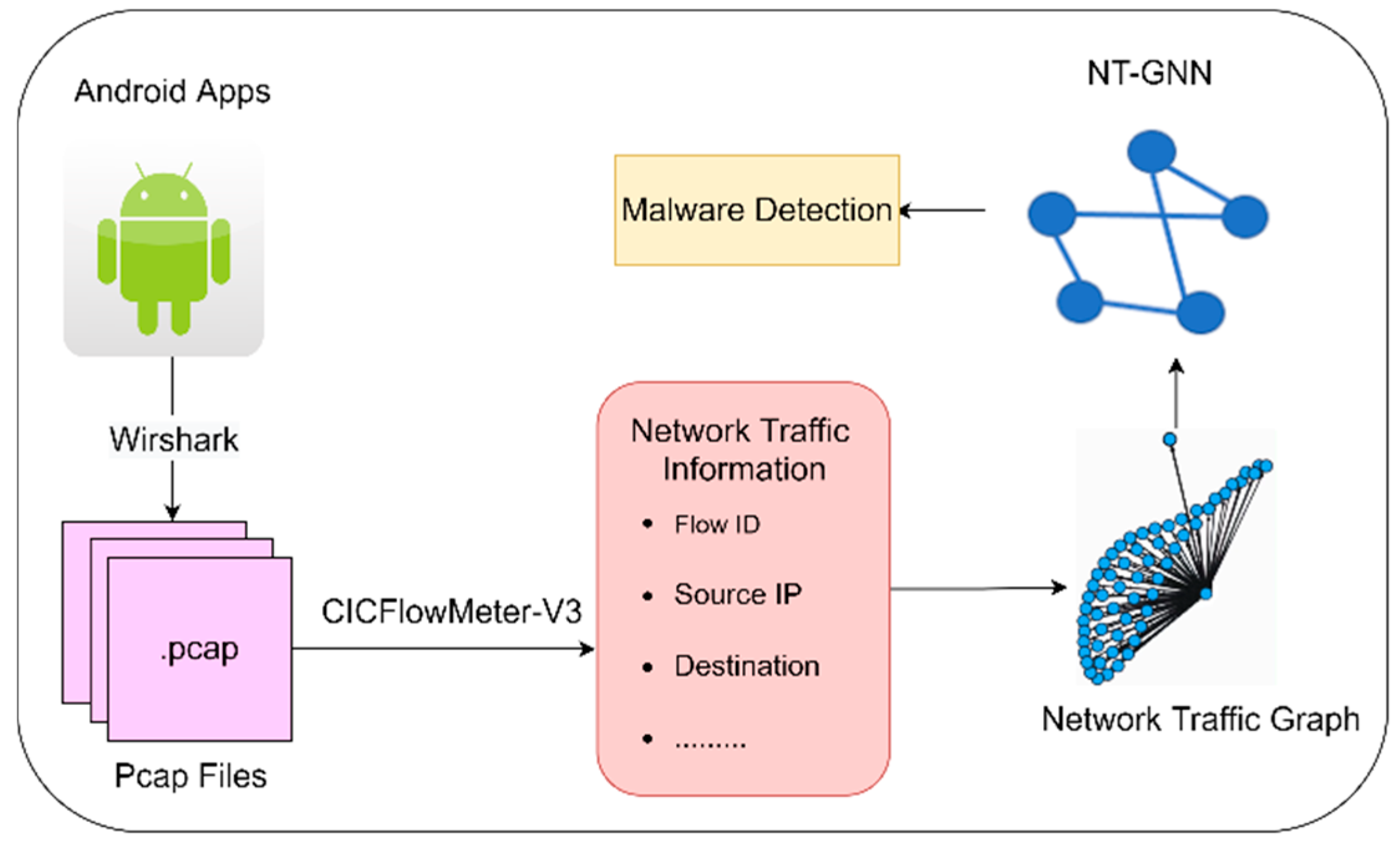
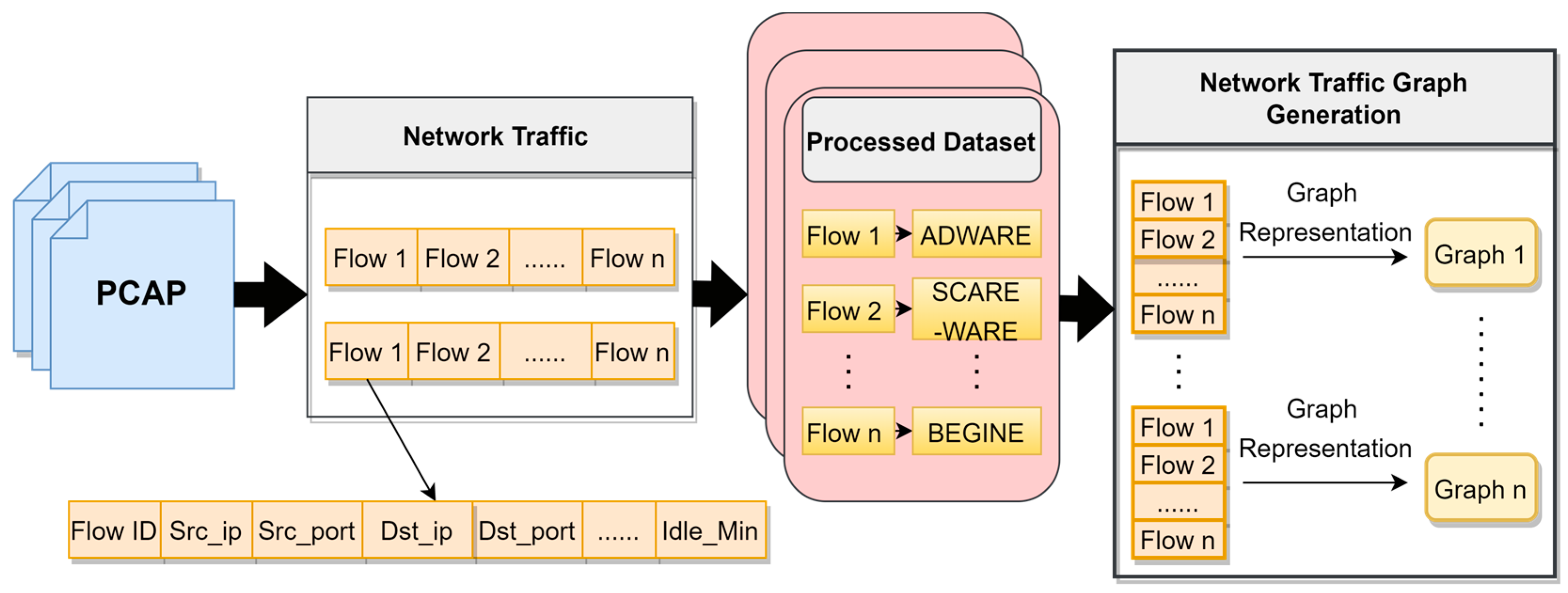
3.1. Extraction of Network Traffic Graph

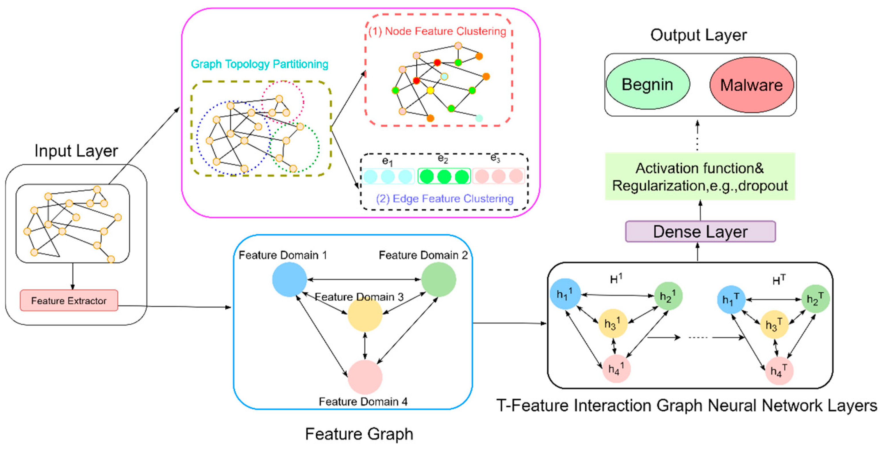
To collect the network traffic created by the execution of the malicious program, we install and execute the Apk application in a real environment and capture the network traffic it creates over time. With programs such as CICFlowMeter-V3 [33], a set of network flows characterized by feature vectors can be retrieved from pcap files. Each flow F has a feature vector $f\in R^m$ attached to it that describes the network traffic between two endpoints over time. After cleaning the data by removing null and zero values, we choose the entire data set to input into the model. From the set of flows that are produced, we let $V=\left\{V_1,\dots ,V_n\right\}$ denotes the set of IP endpoints. We disregard port information and take IP endpoints into account for the main reason; aside from standard ports, port selection is frequently arbitrary, leading to arbitrary and potentially misleading graph structures.

Each pcap traffic packet comprises numerous pieces of traffic $F$ from which the traffic graph can be extracted when the edges represent the methods of communication between these endpoints, and the nodes of the traffic graph represent the network endpoints. Based on our prior research of the expressiveness necessary to accurately capture the traffic patterns of an attack, we construct the expression technique employing each traffic as a node and IP addresses as endpoints of the network traffic graph. This method uses IP addresses as host IDs for two reasons: (1) IP addresses can distinguish between the upstream and downstream properties of flows and may graphically depict the flow relationships between various flows. (2) IP addresses are not randomly selected and contain sufficient data to create a suitable graph structure based on the flows. Figure 2 shows a model graph made from actual data. In more detail, we build a network traffic graph $G=(V,E)$ from a set of flows $F$, where the nodes represent the endpoints engaged in any one of the flows in $F$ and a directed edge is added for all pairs $(s_i,d_i)$ for which a flow $F_i$ exists with source and destination IP $s_i$ and $d_i$, respectively. The feature vector of all flows is combined into the feature vector allocated to this edge $f_i\in {\mathbb{R}}^m$. The mean and standard deviation are used to aggregate the data along this edge, and the 2d-dim feature vector is used to connect the aggregated values for each edge.

The resulting graph depicts the flow of network traffic between the monitored network’s hosts over a specified time period, as well as a clear representation of its structural properties. This graphic shows the monitored network’s structural elements and traffic flow between the hosts over a predetermined time period. It is possible to discern the upstream and downstream properties of the flows, offering a more thorough representation of the linkages in the graphs for individual flows than if the traffic data were treated independently. Consequently, we anticipate that models learning from these graphs will perform considerably better than models identifying individual flows at detection tasks. Our experimental results validate this point.

It should be noted that the IP addresses and traffic in this graph representation are heterogeneous, and the usual GNN model does not support this graph drive well. We redesigned a graph neural network model structure for processing and learning the network traffic graphs retrieved in this section to achieve this goal.

3.2. NT-GNN Model

This section presents the NT-GNN model, a non-standard graph neural network method that takes the network traffic graph and the presence or absence of Android malware as input. NT-GNN model can classify fresh graphs with binary class labels after training in a supervised anomaly detection environment and learning pertinent concepts from the training data (normal vs. abnormal). The traffic graph network model is adapted from the fundamental framework of Message–passing Neural Network (MPNN) [34], which covers most contemporary GNN models.

The entire computation process is carried out along the graph’s structure by the graph neural network, which effectively preserves the graph’s structural information before learning it. Gilmer et al. [34] introduced the universal graph processing architecture known as MPNN, which comprises two primary phases: message–passing and reading. The messaging–passing phase creates information based on the node’s unique properties and transmits it according to the network’s structure. Aggregating neighbor information and updating state information are the next two tasks in this phase. The formula for updating the node’s information and concealed state is as follows.

$$m_{v,i}=m(h_v^t,h_i^t,e_{v,i})$$

(1)

where every node in a graph $G=\left(V,E\right)$ that MPNN operates on has an initial set of features $X_v$ that it uses to encode the first hidden state $h_v^0$ (which is shown as a vector with n elements). Each message–passing iteration is denoted by t, and each node v gets one message $m_{v,i}$, i from each of its neighbors $i=N\left(v\right)$. The edge characteristics of nodes v and i are represented by $e_{v,i}$, while $h_i^t$ is node i’s feature vector at iteration t. After the information has been generated, the node must be modified. Here is the formula for updating nodes.

$$M_v^{t+1}=w\left(\left\{\left\{m_{v,i}|i\in N\left(v\right)\right\}\right.\right)$$

(2)

$$h_v^{t+1}=U\left(h_v^t,M_v^{t+1}\right)$$

(3)

where $w(·)$ is an aggregate function that produces a predetermined output regardless of the number of messages received (i.e., the number of nodes connected). $U(·)$ is the node update function, and it uses the information from $M_v^{t+1}$ and the previous node state $h_v^t$ as input to produce the new node state $h_v^{t+1}$.

The GNN performs a readout phase based on the final hidden states attained after T message–passing iterations. In this situation, the output of the GNN model is generated by passing a subset of hidden states through a programmable readout function, which relies on the particular GNN model. Therefore, the read function’s primary goal is to include the hidden-state embeddings of the final nodes into the model’s output labels. It has the following formula.

$$\widehat{y}=R\left(\right\{h_v^T|v\in G\})$$

(4)

where $\widehat{y}$ is the final output vector, and $R(·)$ is the read function, which has two requirements: (1) to be derivable. (2) to satisfy permutation invariance (the input order of the nodes does not change the final result, which is also to ensure that MPNN has invariance to the graph isomorphism).

The input to our model is a multiple-directed graph $G=(V,E)$, whose nodes can be represented by a host or a flow. Assuming that the initial attributes are $X_j=[x_0,\dots ,x_n]$, the prospective state characteristics of the nodes in the graph often rely on the monitoring data available in the network and require features of a varied kind for initialization. Our model’s representation learning component computes the hidden state features of the graph’s edges and nodes and then generates a hidden state feature vector for each node. $h_j^t$ is the hidden state feature vector of node j at iteration t, and $X_j$ is the initial feature of the node’s hidden state. In this scenario, the initial hidden state of flow j is formed as follows:

$$h_j^0=[x_0,\dots ,x_n,0,0,0\dots ,0]$$

(5)

where the length of the hidden state vector is frequently more than the number of items in the initial feature vector. It should be emphasized that while the possible feature vectors above intuitively explain how the associated endpoints are related to other endpoints in the network, our model is more focused on the network traffic structure, allowing for end-to-end training and improved experimentation. Figure 3 depicts the whole NT-GNN process.

Based on the picture above, we apply the following iterative operations in each messaging $t\in \left[T\right]$:

$$w_j^t=\frac{1}{\left|N\left(j\right)\right|}{\sum }_{i\in N\left(j\right)}{\alpha }_{type}(h_j^t||h_i^t)$$

(6)

In the above equation, ${\alpha }_{type}$ denotes a learnable information function applied on the connection of the hidden states of two linked nodes of the model, i.e., an input graph edge of the NT-GNN model. According to the explanation in the network traffic graph’s extraction section, ${\alpha }_{type}$ automatically comprises two distinct learnable functions: ${\alpha }_s$ for edges ($s\to f$), and ${\alpha }_d$ for edges ($f\to d$). The purpose of the entire formula is to combine the messages calculated on each node using an aggregation function. Since element averaging improves data normalization across numerous messaging rounds, we select it as the message application function.

The node hidden status must be updated after the node information aggregation has been completed. The updated formula is shown here.

$$h_j^{t+1}={\beta }_{type}(h_j^t||w_j^t)$$

(7)

where ${\beta }_{type}$ is the update function applied to the current concealed states of aggregated nodes and messages. As with the message’s function, ${\delta }_{type}$ consists of two distinct learnable functions (${\beta }_e$ and ${\beta }_f$) that are used to change the hidden states of nodes and flows, respectively.

Consequently, the ${\alpha }_s$, ${\alpha }_d$, ${\beta }_e$, and ${\beta }_f$ functions are all learnable functions that neural networks may approximate during training. ${\alpha }_s$ and ${\alpha }_d$ are implemented as two-layer fully connected neural networks in our model, whereas ${\beta }_e$ and ${\beta }_f$ are represented as gated recurrent units (GRUs [35]). To activate all of the layers between the various NNs stated above, we utilize the ReLU activation function. We define the function as follows:

$$ReLU\left(x\right)=max(0,x)$$

(8)

After aggregating node information and updating the hidden state, the final step is to read the function definition.

$$y_j=R\left(h_j^T\right)$$

(9)

The function $R(·)$ accepts the final concealed state of each flow as its argument and returns the anticipated category for that flow (either malicious or benign flows). This component is constructed with a three-layer fully connected neural networks, and one hot encoding is used to produce the potential output volume classes. We employ the softmax activation function for the $R(·)$ function in the last layer instead of the ReLU activation function previously discussed. Here is the softmax function formula.

$${softmax\left(x\right)}_j=\frac{exp\left(x_j\right)}{{\sum }_{k}exp\left(x_k\right)}$$

(10)

To prevent gradient dispersion, which lowers the learning rate during gradient descent computations, the NT-GNN model in the article utilizes a cross-entropy loss function. It has the following formula.

$$Loss=-[y\mathit{log}\widehat{y}+(1-y\left)\mathit{log}(1-\widehat{y})\right]$$

(11)

Here, $y$ is the true label value (Positive class values are 1, whereas negative class values are 0.) and $\widehat{y}$ is the predicted rate value ($\widehat{y}\in \left(\mathrm{0,1}\right)$). It characterizes the distinction between the actual sample label and the predicted probability.

4. Experiment and Results

In this part, we describe the datasets and the experimental setup in detail. Then, the evaluation metrics are introduced, and finally, we compare the detection results of the NT-GNN model using network traffic graphs and the detection results of deep learning models with other feature extraction methods.

4.1. Experimental Setup

We used a Windows 10-based operating system with Intel(R) i7-11700 CPU with 32 GB of RAM, GeForce RTXTM 3090 Ti GPU to deploy NT-GNN. GPU is used to speed up the neural network model’s training process because the model contains a lot of data. We use several packages for Python to implement the proposed method: CICFlowMeter-V3, NetworkX, TensorFlow, and Matplotlib. On top of this equipment setup, the NT-GNN model takes 36 h to run the entire data. The same data imported into the DT model takes 42 h to run, the RF model takes 38 h, and the CNN takes 37.5 h.

4.2. Datasets

We utilized two openly accessible datasets, CICAndMal2017 [24] and AAGM [36], to evaluate our method realistically and accurately. The CICAndMal2017 dataset was created by running malicious and benign apps on smartphones, avoiding the behavior of more sophisticated malware samples that alter their behavior to generate erroneous results when they recognize the emulator environment at runtime. On actual devices, the researchers installed 5000 symptoms (426 malicious and 5065 benign samples), gathered data for each sample in three states (overcoming the invisibility of sophisticated malware), and documented network traffic characteristics to construct the datasets. Currently, the full datasets comprise 2126 samples and 2,583,878 network traffic, each representing an instance of an Android application loaded on a mobile device. During the run, network flows for each sample are collected. A total of 84 characteristics were captured for each network flow. Each of these samples contains three labels: (1) a binary label stating whether the sample is dangerous or not, (2) a category label with five potential values indicating the specific type of malware, and (3) a family label with 42 possible values identifying the specific family of malware. The precise categories of the CICAndMal2017 datasets are detailed in

Table 1. CICAndMal2017 datasets specific categories.

Category	Family Tree
Benign	Benign2015		Benign2016		Benign2017
Malware	Adware	Dowgin	Ewind	Feiwo	Gooligan	Kemoge
		koodous	Mobidash	Selfmite	Shuanet	Youmi
	Ransomware	Charger	Jisut	Koler	LockerPin	Simplocker
		Pletor	PornDroid	RansomBO	Svpeng	WannaLocker
	Scareware	FakeAV	AndroidSpy	AVpass	AVAndroid	FakeApp
		Penetho	VirusShield	FakeJobOffer	FakeTaoBao	FakeAppAL
		AndroidDefender
	SMSMalware	BeanBot	Biige	FakeInst	FakeMart	FakeNotify
		Jifake	Mazarbot	Zsone	Plankton	SMSsniffer
		Nandrobox

. Since this is a detection job, only binary labels are employed.

We also carried out malware detection tasks on the AAGM dataset to more accurately reflect the performance of the methods in this paper. The AAGM dataset also installs Android apps on actual devices and records sample traffic while they are in use, avoiding the behavior of sophisticated Android malware that would otherwise recognize the emulator and react. There are 1900 samples total in this collection, 1500 of which are good software and 400 malware. CICFlowMeter-V3 with 84 features was used to extract network traffic for each sample. Each sample has three labels, similar to the previous datasets, and

Table 2. AAGM datasets specific categories.

Category	Family Tree
Benign	Benign2015		Benign2016
Malware	Adware	Airpush	Dowgin	Kemoge
		Mobidash	Shuanet
	General Malware	AVpass	FakeAV	FakeFlash
		GGtracker	Penetho

lists their precise classifications.

In the paper, each sample needs to be cleaned before entering the network traffic graph extraction by removing the null and outlier values. Then, the cleaned data set is normalized by converting the timestamp and IP address into the numerical format, and finally, each sample enters the network traffic graph extraction session. There are 4026 samples and 3,445,000 flows, and the data size is about 40 GB.

We adhere to a rigid evaluation procedure to provide a fair and unbiased comparison. First, we divide the datasets into training, test, and validation sets, and evaluate our model on them. Then the model is trained on the training data set, hyperparameters are selected based on the performance of grid search for the validation set, and the outcomes are given on the test set utilizing the best hyperparameters. Finally, our experiments show the average results of the 10-fold cross-validation.

4.3. Evaluation Metrics

The NT-GNN model is an ML model in which malware detection is a classification issue. This research uses the following assessment measures to analyze the ML model’s performance. We determined the values for True Negatives (TN), True Positives (TP), False Negatives (FN), and False Positives (FP). True Negatives (TN) indicate the right classification of benign applications as benign. True Positives (TP) are the number of malware programs that have been accurately recognized as harmful. False Negatives (FN) are the number of malware samples that have been incorrectly categorized as benign. False Positives (FP) represent the number of benign apps that were wrongly identified as malicious software.

Accuracy is the proportion of samples properly categorized by the model relative to the overall sample count of a given test data set. This is how the formula is displayed:

$$Accuracy=\frac{TP+TN}{TP+TN+FN+FP}$$

(12)

Precision is the percentage of samples with positive prediction results that are right. The equation reads as follows:

$$Precision=\frac{TP}{TP+FP}$$

(13)

Recall that relates to the fraction of projected positive samples among the total positive samples. The formula for calculating is:

$$Recall=\frac{TP}{TP+TN}$$

(14)

F1-Score is a mix of accuracy and memory. When one variable rises, the other must decrease proportionally. To harmonize the 2 metrics, F1-Score is made available:

$$F-measure=\frac{2\times precision\times recall}{precision+recall}$$

(15)

The receiver-operating characteristic (ROC) curve is sometimes referred to as the curve of receptivity. The curve’s vertices represent the reaction to the identical signal stimulus, but the results are derived using various evaluative standards. They create the curve by fusing the points using the rate of erroneous positives (FPR) as the X coordinate and the true positive rate (TPR) as the Y coordinate.

$$FPR=\raisebox{1ex}{$FP$}\!\left/ \!\raisebox{-1ex}{$FP+TN$}\right.$$

(16)

$$TPR=\raisebox{1ex}{$TP$}\!\left/ \!\raisebox{-1ex}{$TP+FN$}\right.$$

(17)

The precision-recall (PR) curve is the line generated by joining Recall as the X coordinate and Precision as the Y coordinate are two points. It serves to assess the classification performance of ML algorithms for given datasets. It correlates ROC curves spatially when the recall is greater than 0, and their confusion matrices are the same.

The area under the curve (AUC) is a crucial gauge of how well a classifier performs and is regarded as the region beneath the ROC curve. When the value is closer to 1, the detection method’s authenticity is greater; when it reaches 0.5, its veracity is at its smallest and it is useless. The calculation formula is given below.

$$AUC=\frac{\sum _{iϵpositiveClass}{rank}_i-\frac{M(1+M)}{2}}{M\times N}$$

(18)

The Kappa coefficient is a statistic for assessing the accuracy of the categorization as well as its consistency. This coefficient may be used to determine if the classification results obtained and the model predictions for the classification issue are consistent. The confusion matrix, which accepts values between −1 and 1 and is typically larger than 0, is used to determine the kappa coefficient. The formula for calculating is

$$kappa=\frac{p_0-p_e}{1-p_e}$$

(19)

where $p_e$ stands for the chance of consistency errors and $p_0$ stands for the overall classification accuracy.

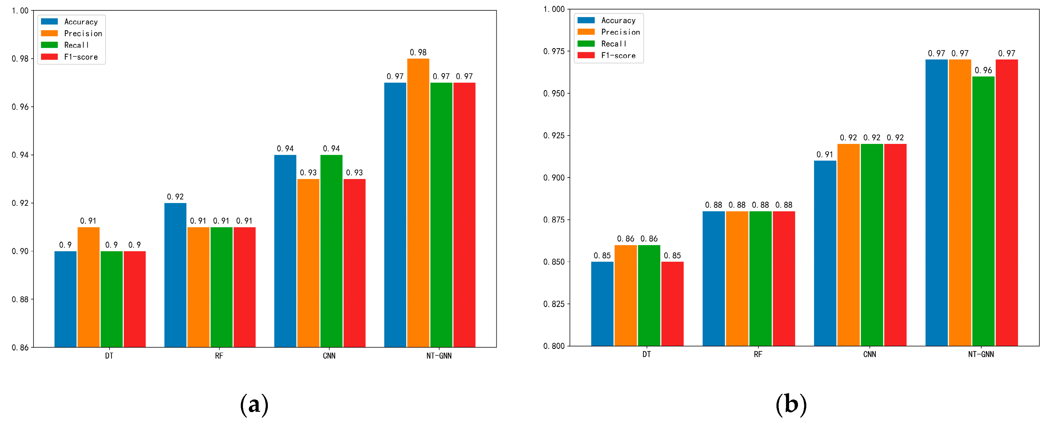
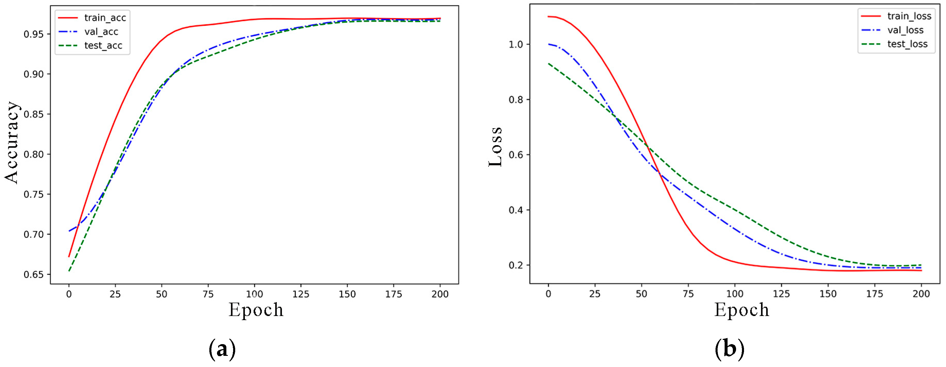
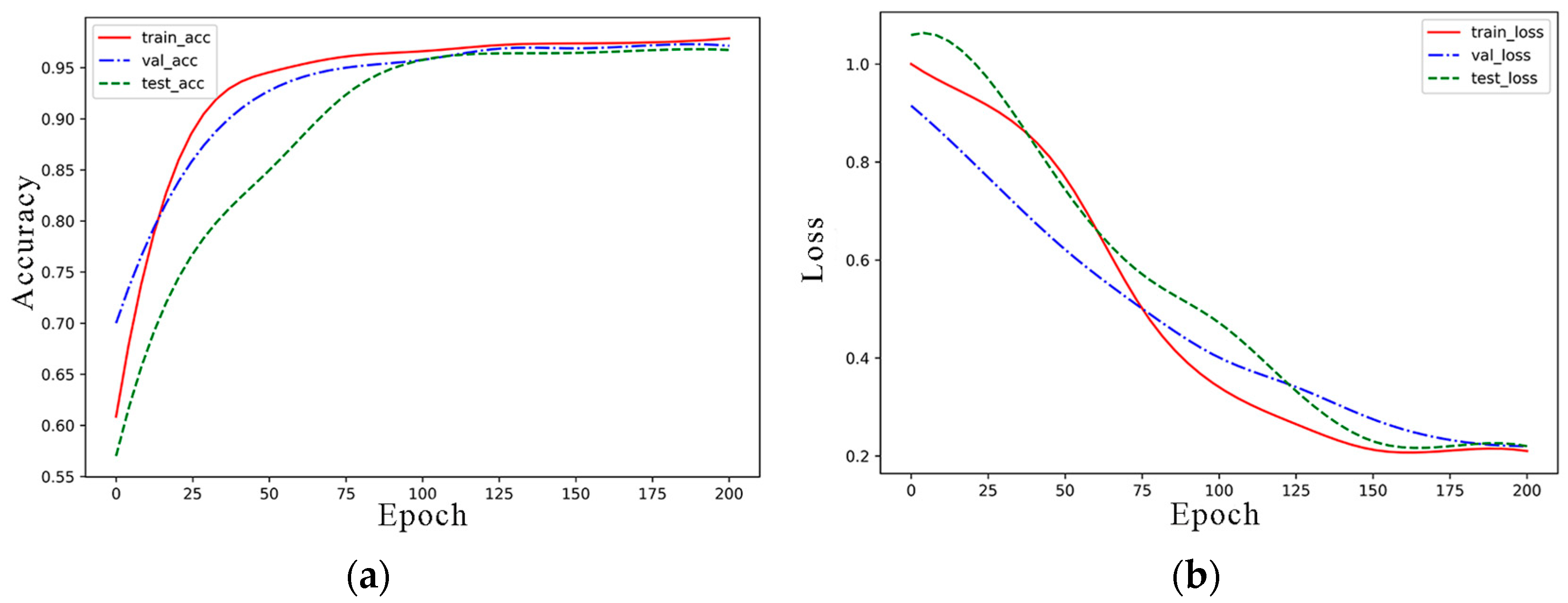
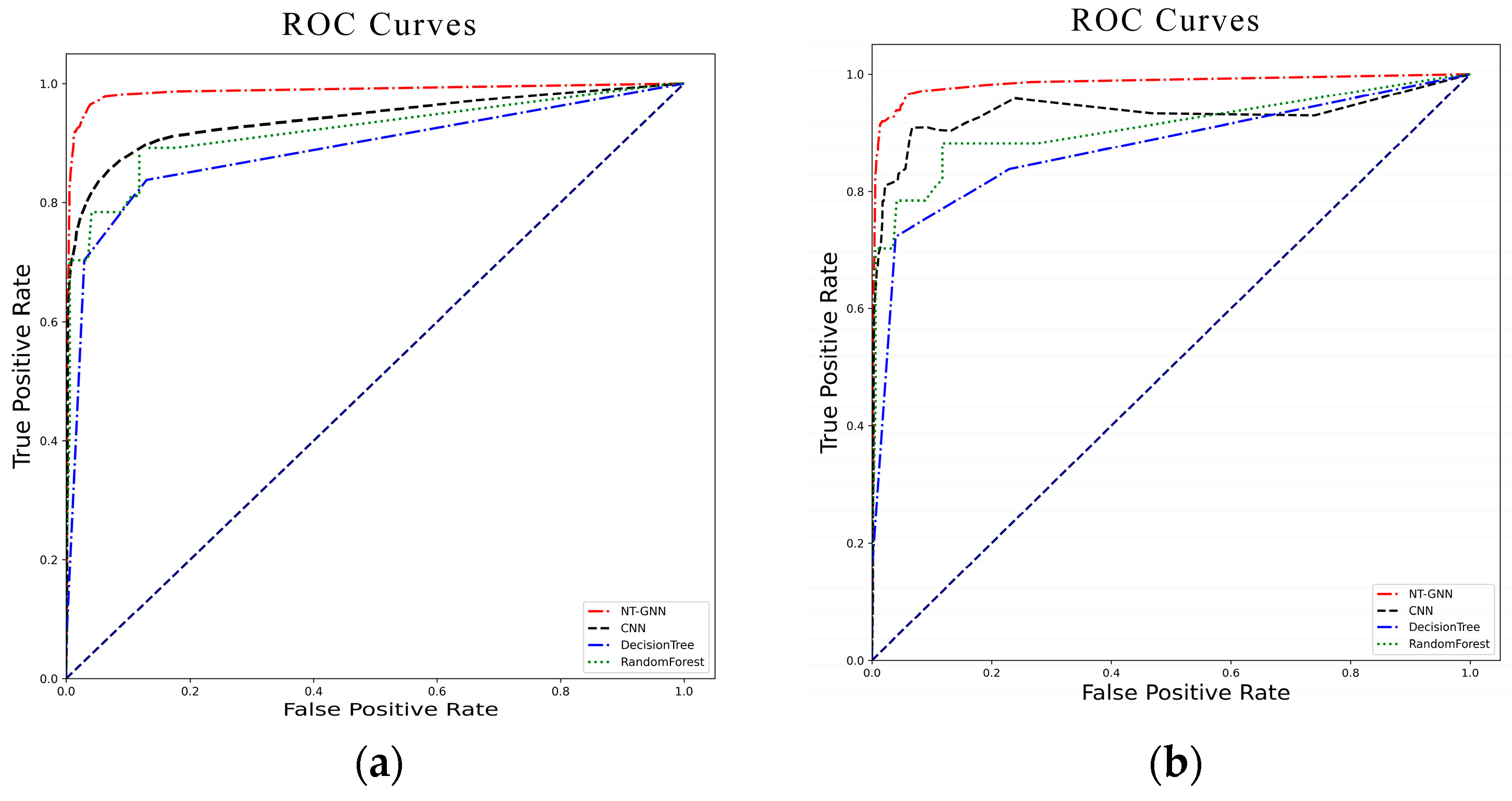
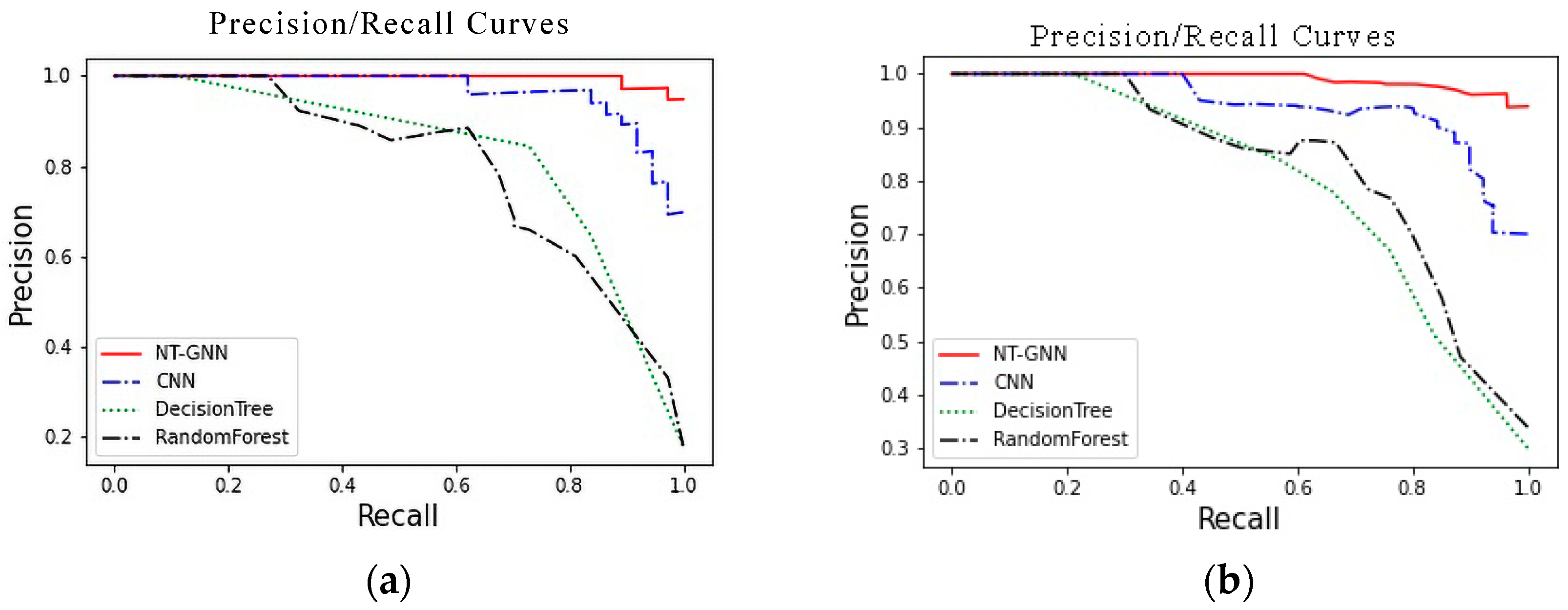
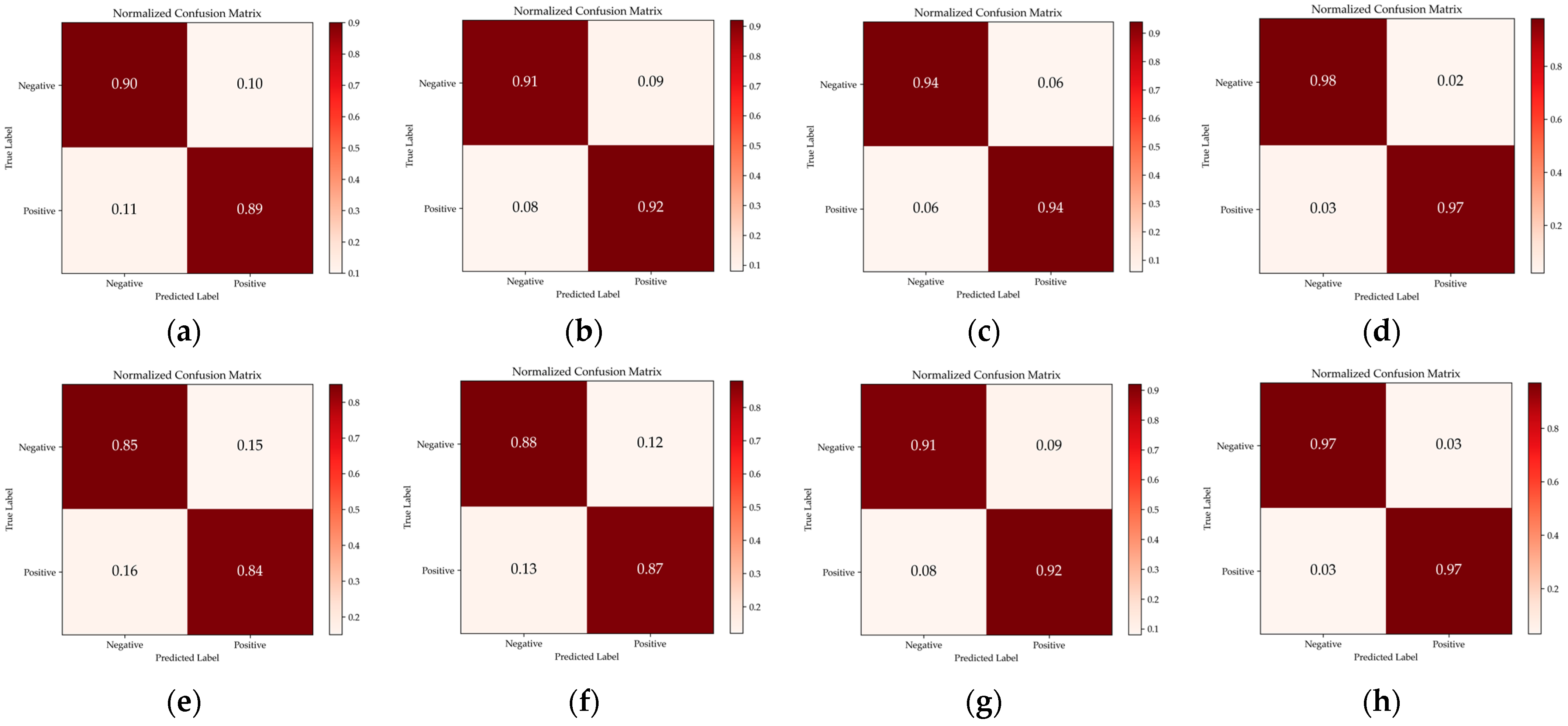
4.4. Experimental Results

This section focuses on the model’s performance in this paper and compares it to the DecisionTree (DT), Random Forest (RF), Convolutional Neural Network (CNN) models. DT is a widely used classifier with a simple structure and fast efficiency. RF is a type of integrated learning in which numerous poor classifiers are combined to get good results. CNN is a typical deep neural network model, which can be tuned by parameters to train a huge amount of data and get good performance. The better the model performs, the higher the accuracy, precision, recall, and F1 score values.

Table 3. Performances of five models in CICAndMal2017.

Model	Accuracy	Precision	Recall	F1-Score
DT	0.90	0.91	0.90	0.90
RF	0.92	0.91	0.91	0.91
CNN	0.94	0.93	0.94	0.93
NT-GNN	0.97	0.98	0.97	0.97

shows each ML model’s two-classifier performance on the CICAndMal2017 test datasets. The findings show that the proposed model performs greater overall than the ML and CNN models that are more often used. The four assessment indicators showed that the NT-GNN model performed the best. For example, while traditional ML techniques and CNN can achieve accuracy and precision values of 0.90 and higher, the NT-GNN described in this research can achieve accuracy and precision values of 0.97 and 0.98.

Table 4. Performances of five models in AAGM.

Model	Accuracy	Precision	Recall	F1-Score
DT	0.85	0.86	0.86	0.85
RF	0.88	0.88	0.88	0.88
CNN	0.91	0.92	0.92	0.92
NT-GNN	0.97	0.97	0.96	0.97

displays the performance of two classifiers using the NT-GNN, DT, RF, and CNN models on the test datasets of AAGM. It is clear from this table that the NT-GNN model had a recall and accuracy of 0.96 and 0.97, respectively.

In contrast, the recall value (0.86) and accuracy (0.85) of DT; and the accuracy, precision, recall, and F1-score values (0.88) of RF were compared. In summary, the NT-GNN model outperforms the other three models on the CICAndMal2017 dataset as well as the other three models on the AAGM dataset. Because of their power to digest raw data formats and capacity to learn characteristics, graph neural networks are increasingly being employed for malware detection.

The performance of the DT, RF, CNN, and NT-GNN models is more clearly reflected in their result distributions, shown in Figure 4.

To better demonstrate the model’s advantages in this paper, we assess the effectiveness of the NT-GNN model compared to other cutting-edge approaches. It is important to note that these articles use either the CICAndMal2017 datasets or the AAGM datasets. The NT-GNN model classified malware binary files with the best accuracy (0.97) and precision (0.98), as shown in

Table 5. Performance of the proposed method in CICAndMal2017.

Prediction Method	Model	Accuracy	Precision	Recall	F1-Score
Guo [23]	CNN	0.94	0.91	0.95	-
Gohari [25]	CNN-LSTM	0.95	0.97	0.93	0.95
Xu [31]	Hybrid-Falcon	0.96	0.96	0.96	0.96
Zhu [37]	MSerNetDroid	0.96	0.98	0.97	0.96
Our Model	NT-GNN	0.97	0.98	0.97	0.97

. This graph neural network model with network traffic graph displays superior performance than CNN or other deep learning techniques. NT-GNN achieves an accuracy of 0.97; other research [23,25,31,37] obtained precisions of 0.94, 0.95, 0.96, and 0.96, respectively. As seen from

Table 6. Performance of the proposed method in AAGM.

Prediction Method	Model	Accuracy	Precision	Recall	F1-Score
Lashkari [36]	AE	0.57	0.41	0.66	0.51
Xu [31]	Hybrid-Falcon	0.96	0.95	0.97	0.96
Zhu [37]	MSerNetDroid	0.94	0.94	0.94	0.94
Our Model	NT-GNN	0.97	0.97	0.96	0.97

, the precision of the NT-GNN model for malware detection in the AAGM datasets reached 0.97, while other studies [31,36,37] achieved 0.96, 0.57, and 0.94, respectively. It can be seen that NT-GNN is very effective on the AAGM datasets.

To more visually demonstrate the efficiency of the NT-GNN model in malware classification, Figure 5 and Figure 6 show the accuracy and loss curves of NT-GNN on the training, testing, and validation datasets. In binary classification (2 classifiers), NT-GNN achieves an impressive accuracy of 97.44%, 97.36%, and 97.38% in the training, testing, and validation samples of CICAndMal2017, respectively (Figure 5a); the loss of binary classification is 1.230789423~0.200601578 in the training sample, 0.934191~0.208033 in the testing sample and the validation sample is 1.052714944~0.202082589 (Figure 5b).

The above figures show the current model’s performance on the public datasets of CICAndMal2017. To better verify the performance of the model in this research, we will show the accuracy and loss curves on the AAGM datasets. In the detector, NT-GNN achieves 97.18%, 97.13%, and 97.15% accuracy in the training, testing, and validation samples, respectively (Figure 6a); its loss is 1.089524388~0.216055843 in the training sample, 1.059389~0.2207491 in the testing sample, and 0. 915076~ 0.219921 in the validation sample (Figure 6b).

Figure 7 and Figure 8 display the ROC and PR curves to illustrate the benefits of NT-GNN. The ROC curves of the four models are displayed in Figure 7. Where Figure 7a depicts the ROC curves of the four models on the CICAndMal2017 datasets, and Figure 7b shows the ROCcurves of the four methods on the AAGM datasets. AUC is the area underneath the ROC curve. The classification is more effective the bigger the AUC. The AUC value of NT-GNN in Figure 7a is 0.97, which is much higher than DT, RF, and CNN. In Figure 7b, the AUC value of DT is 0.85, while the AUC score of NT-GNN is 0.97. Consequently, NT-GNN will be a valuable classification device for malware, or at the very least, a supplement to existing approaches. Figure 8 illustrates the link between accuracy and recall through the PR curves of the four ML models on the CICAndMal2017 and AAGM datasets. Precision and recall curve plots were utilized to evaluate categorization performance. When there is little difference between positive and negative samples, the trends of the ROC curve and the PR curve are similar; nevertheless, when several samples are negative, both curves diverge significantly. The ROC impact still appears favorable, but the PR reflects the overall effect. Figure 7 and Figure 8 demonstrate that the NT-GNN model provides the optimum performance.

The TP and FN rates of malware categorization form the confusion matrix value. The anticipated categorization by the NN is shown along the axis horizontal of the matrix of perplexity. The number on the diagonal line denotes the number of accurate classifications made by the neural network, while the vertical coordinate denotes the actual detection. The number that is shown outside of the diagonal indicates some discrepancies that exist between the projected and observed classifications. This number also represents the number of inaccurate classifications produced by the neural network. The results of the confusion matrix analysis performed for the malware detector (NT-GNN) as well as the DT, RF, and CNN models on the CICAndMal2017 and AAGM datasets are redisplayed in Figure 9. The findings of the confusion matrix indicate that the NT-GNN model does a good job on the datasets. According to the confusion matrix, we also computed the coefficient of Kappa to assess the method’s influence on binary classification, which will help better illustrate the model outcomes. The Kappa coefficient value for malware detection is 0.97 on both the CICAndMal2017 datasets and the AAGM datasets.

5. Discussion and Conclusions

This paper suggests a network traffic graph-based method (NT-GNN) for detecting Android malware. The detection performance of the present model was evaluated and contrasted with other models using the CICAndMal2017 and AAGM datasets. Additionally, we analyze our graph neural network model using a ten-rule cross-validation method to reflect the model performance in this research accurately. Ten-fold in cross-validation, the dataset is split into 10 equal parts, with each part being used alternately as training data and test data for experiments. The results of each experiment are averaged to get the proper rate for the datasets. The goal of cross-validation is to improve the accuracy and reliability of the tested models. Cross-validation is used to check the predicted performance of models, particularly trained models on new data, to develop trustworthy and stable models. By using cross-validation, overfitting can be minimized to some extent.

Compared to other DL approaches, NT-GNN has a detection accuracy, precision, recall, and F1 score of 0.97, 0.98, 0.97, and 0.97 for most malware, as shown in Table 3, Table 4, Table 5 and Table 6. In this study, the CICAndMal2017 and AAGM datasets were utilized to verify the detection performance of the NT-GNN model, and positive experimental findings were achieved.

The graph representation module of the traffic network graph describes the attack patterns of network traffic data more precisely, accurately captures the structural features of malware network traffic, and illustrates the variety and specificity of the malware detection challenge. Regularization is also used to accelerate the convergence of the training of the deep model, which occurs in around 200 epochs. In conclusion, the NT-GNN model suggested in this article successfully detects Android malware.

Following this, we shall perform experiments on the following lines of inquiry. One of our goals for the future is to use the NT-GNN model to classify Android malware and determine their malware classes and families. Another direction is to extract the dataset’s static and dynamic features, use different graph representation models for malware dataset detection, and compare them with the proposed NT-GNN model to prove its advancement.

References

1. Guan, X.H.; Liu, T.; Liu, J.; Yu, L. Android malware detection: A survey. Sci. Sin. Inform. 2020, 50, 1148–1177. [Google Scholar]
2. Fiky, A.H.E.; Elshenawy, A.; Madkour, M.A. Detection of Android Malware using Machine Learning. In Proceedings of the 2021 International Mobile, Intelligent, and Ubiquitous Computing Conference, Cairo, Egypt, 26–27 May 2021. [Google Scholar]
3. Almahmoud, M.; Alzu’bi, D.; Yaseen, Q. ReDroidDet: Android malware detection based on recurrent neural network. Proc. Comp. Sci. 2021, 184, 841–846. [Google Scholar] [CrossRef]
4. Arvind, M.; Sangal, A.L. MLDroid—Framework for Android malware detection using machine learning techniques. Neural. Comput. Appl. 2021, 33, 5183–5240. [Google Scholar]
5. Liu, K.J.; Xu, S.W.; Xu, G.A.; Zhang, M.; Sun, D.W.; Liu, H.F. A review of android malware detection approaches based on machine learning. IEEE Access 2020, 8, 124579–124607. [Google Scholar] [CrossRef]
6. Kabakus, A.T. DroidMalwareDetector: A novel Android malware detection framework based on convolutional neural network. Expert Syst. Appl. 2022, 206, 117833. [Google Scholar] [CrossRef]
7. Musikawan, P.; Kongsorot, Y.; You, I.; So-In, C. An enhanced deep learning neural network for the detection and identification of Android malware. IEEE Internet Things J. 2022, 1, 1. [Google Scholar] [CrossRef]
8. Kim, T.G.; Kang, B.J.; Mina, R.; Sezer, S.; Im, E.G. A multimodal deep learning method for android malware detection using various features. IEEE Trans. Inf. Forensics Secur. 2018, 14, 773–788. [Google Scholar] [CrossRef]
9. Li, J.; Sun, L.C.; Yan, Q.B.; Li, Z.Q.; Srisa-An, W.; Ye, H. Significant permission identification for machine-learning-based android malware detection. IEEE Trans. Industr. Inform. 2018, 14, 3216–3225. [Google Scholar] [CrossRef]
10. Karbab, E.B.; Debbabi, M.; Derhab, A.; Mouheb, D. MalDozer: Automatic framework for android malware detection using deep learning. Digit. Investig. 2018, 24, S48–S59. [Google Scholar] [CrossRef]
11. Abdurrahman, P.; Acarman, T. Deep learning for effective Android malware detection using API call graph embeddings. Soft Comput. 2020, 24, 1027–1043. [Google Scholar]
12. Vasileios, S.; Geneiatakis, D. On machine learning effectiveness for malware detection in Android OS using static analysis data. J. Inf. Secur. Appl. 2021, 59, 102794. [Google Scholar]
13. Molina-Coronado, B.; Mori, U.; Mendiburu, A.; Miguel-Alonso, J. Towards a fair comparison and realistic evaluation framework of android malware detectors based on static analysis and machine learning. Comput. Secur. 2023, 124, 102996. [Google Scholar] [CrossRef]
14. Bai, H.P.; Xie, N.N.; Di, X.Q.; Ye, Q. Famd: A fast multifeature android malware detection framework, design, and implementation. IEEE Access 2020, 8, 194729–194740. [Google Scholar] [CrossRef]
15. He, K.; Kim, D.S. Malware detection with malware images using deep learning techniques. In Proceedings of the 2019 18th IEEE International Conference on Trust, Security And Privacy In Computing And Communications, Rotorua, New Zealand, 5–8 August 2019. [Google Scholar]
16. Xu, K.; Li, Y.J.; Deng, R.; Chen, K.; Xu, J.Y. Droidevolver: Self-evolving android malware detection system. In Proceedings of the 2019 IEEE European Symposium on Security and Privacy, Stockholm, Sweden, 17–19 June 2019. [Google Scholar]
17. Chen, R.; Li, Y.Y.; Fang, W.W. Android malware identification based on traffic analysis. In Proceedings of the International Conference on Artificial Intelligence and Security, New York, NY, USA, 26–28 July 2019. [Google Scholar]
18. Wu, Z.H.; Pan, S.R.; Chen, F.W.; Long, G.D.; Zhang, C.Q.; Yuphilip, S. A comprehensive survey on graph neural networks. IEEE Trans. Neural Netw. Learn. Syst. 2020, 32, 4–24. [Google Scholar] [CrossRef] [Green Version]
19. Rahali, A.; Lashkari, A.H.; Kaur, G.; Taheri, L.; Gagnon, F.; Massicotte, F. Didroid: Android malware classification and characterization using deep image learning. In Proceedings of the 2020 The 10th International Conference on Communication and Network Security, New York, NY, USA, 27–29 November 2020. [Google Scholar]
20. Alzaylaee, M.K.; Suleiman, Y.Y.; Sakir, S. DL-Droid: Deep learning based android malware detection using real devices. Comput. Secur. 2020, 101663. [Google Scholar] [CrossRef]
21. Lotfollahi, M.; Siavoshani, M.J.; Zade, R.S.H.; Saberian, M. Deep packet: A novel approach for encrypted traffic classification using deep learning. Soft Comput. 2019, 24, 1999–2012. [Google Scholar] [CrossRef]
22. Feng, J.Y.; Shen, L.M.; Chen, Z.; Wang, Y.Y.; Li, H. A two-layer deep learning method for android malware detection using network traffic. IEEE Access 2020, 8, 125786–125796. [Google Scholar] [CrossRef]
23. Guo, Y.M.; Zhang, A.X. Classification Method of Android Traffic based on Convolutional Neural Network. Comm. Technol. 2020, 53, 432–437. [Google Scholar]
24. Lashkari, A.H.; Kadir, A.F.A.; Laya, T.; Ghorbani, A.A. Toward developing a systematic approach to generate benchmark android malware datasets and classification. In Proceedings of the 2018 International Carnahan Conference on Security Technology, Montreal, QC, Canada, 22–25 October 2018. [Google Scholar]
25. Mahshid, G.; Hashemi, S.; Abdi, L. Android malware detection and classification based on network traffic using deep learning. In Proceedings of the 2021 7th International Conference on Web Research, Tehran, Iran, 19–20 May 2021. [Google Scholar]
26. Abuthawabeh, M.; Kamel, A.; Khaled, W.M. Android malware detection and categorization based on conversation-level network traffic features. In Proceedings of the 2019 International Arab Conference on Information Technology, Al Ain, United Arab Emirates, 3–5 December 2019. [Google Scholar]
27. John, T.S.; Thomas, T.; Emmanuel, S. Graph convolutional networks for android malware detection with system call graphs. In Proceedings of the 2020 Third ISEA Conference on Security and Privacy, Guwahati, India, 27 February 2020–1 March 2020. [Google Scholar]
28. Gao, H.; Cheng, S.Y.; Zhang, W.M. GDroid: Android malware detection and classification with graph convolutional network. Comput. Secur. 2021, 106, 102264. [Google Scholar] [CrossRef]
29. Hei, Y.M.; Yang, R.Y.; Peng, H.; Wang, L.H.; Xu, J.W.; Liu, H.; Xu, J.; Sun, L.C. Hawk: Rapid android malware detection through heterogeneous graph attention networks. IEEE Trans. Neural Netw. Learn. Syst. 2021, 1–15. [Google Scholar] [CrossRef]
30. Lo, W.W.; Layeghy, S.; Sarhan, M.; Gallagher, M.; Portmann, M. Graph Neural Network-based Android Malware Classification with Jumping Knowledge. In Proceedings of the 2022 IEEE Conference on Dependable and Secure Computing (DSC), Edinburgh, UK, 22–24 June 2022. [Google Scholar]
31. Xu, P.; Eckert, C.; Zarras, A. hybrid-Flacon: Hybrid Pattern Malware Detection and Categorization with Network Traffic andProgram Code. arXiv 2021, arXiv:2112.100352112. [Google Scholar]
32. Busch, J.; Kocheturov, A.; Tresp, V.; Seidl, T. NF-GNN: Network flow graph neural networks for malware detection and classification. In Proceedings of the 33rd International Conference on Scientific and Statistical Database Management, New York, NY, USA, 11 August 2021. [Google Scholar]
33. Lashkari, A.H.; Draper-Gil, G.; Mamun, M.; Ghorbani, A.A. Characterization of encrypted and vpn traffic using time-related. In Proceedings of the 2nd International Conference on Information Systems Security and Privacy, Rome, Italy, 19–21 February 2016. [Google Scholar]
34. Gilmer, J.; Schoenholz, S.S.; Riley, P.F.; Vinyals, O.; Dahl, G.E. Neural message passing for quantum chemistry. In Proceedings of the 34th International Conference on Machine Learning, Sydney, Australia, 6–11 August 2017; Volume 70, pp. 1263–1272. [Google Scholar]
35. Chung, J.Y.; Gulcehre, C.; Cho, K.H.; Bengio, Y. Empirical evaluation of gated recurrent neural networks on sequence modeling. arXiv 2014, arXiv:1412.35551412. [Google Scholar]
36. Lashkari, A.H.; Kadir, A.F.A.; Gonzalez, H.; Mbah, K.F.; Ghorbani, A.A. Towards a network-based framework for android malware detection and characterization. In Proceedings of the 2017 15th Annual Conference on Privacy, Security and Trust, Calgary, AB, Canada, 28–30 August 2017. [Google Scholar]
37. Zhu, H.J.; Gu, W.; Wang, L.M.; Xu, Z.C.; Sheng, V.S. Android malware detection based on multi-head squeeze-and-excitation residual network. Expert Syst. Appl. 2023, 212, 118705. [Google Scholar] [CrossRef]
Figure 1. The overall architecture of the proposed model.
Electronics 12 00789 g001
Figure 2. Network traffic graph extraction process.
Electronics 12 00789 g002
Figure 3. The schematic depiction of the NT-GNN model.
Electronics 12 00789 g003
Figure 4. The results of the ten-fold cross-test for the DT, RF, CNN, and NT-GNN models. (a) Performances of four models on CICAndMal2017. (b) Performance of the four models on AAGM.
Electronics 12 00789 g004
Figure 5. (a) Accuracy and (b) loss curves of the NT-GNN model in CICAndMal2017.
Electronics 12 00789 g005
Figure 6. (a) Accuracy and (b) loss curves of the NT-GNN model in AAGM.
Electronics 12 00789 g006
Figure 7. ROC curves for the four models to detect malicious software. (a) ROC curves of the four models on CICAndMal2017. (b) ROC curves of the four models on AAGM.
Electronics 12 00789 g007
Figure 8. PR curves for the four models to detect malware. (a) PR curves of the four models on CICAndMal2017. (b) PR curves of the four models on AAGM.
Electronics 12 00789 g008
Figure 9. Confusion matrix performance. (ad) are the confusion matrices of DT, RF, CNN, and NT-GNN models on CICAndMal2017. (eh) are the confusion matrices of DT, RF, CNN, and NT-GNN models on AAGM.
Electronics 12 00789 g009