An Approach for Classification of Alzheimer’s Disease Using Deep Neural Network and Brain Magnetic Resonance Imaging (MRI)

Abstract

Alzheimer’s disease (AD) is a deadly cognitive condition in which people develop severe dementia symptoms. Neurologists commonly use a series of physical and mental tests to diagnose AD that may not always be effective. Damage to brain cells is the most significant physical change in AD. Proper analysis of brain images may assist in the identification of crucial bio-markers for the disease. Because the development of brain cells is so intricate, traditional image processing algorithms sometimes fail to perceive important bio-markers. The deep neural network (DNN) is a machine learning technique that helps specialists in making appropriate decisions. In this work, we used brain magnetic resonance scans to implement some commonly used DNN models for AD classification. According to the classification results, where the average of multiple metrics is observed, which includes accuracy, precision, recall, and an F1 score, it is found that the DenseNet-121 model achieved the best performance (86.55%). Since DenseNet-121 is a computationally expensive model, we proposed a hybrid technique incorporating LeNet and AlexNet that is light weight and also capable of outperforming DenseNet. To extract important features, we replaced the traditional convolution Layers with three parallel small filters ($1\times 1,3\times 3$, and $5\times 5$). The model functions effectively, with an overall performance rate of 93.58%. Mathematically, it is observed that the proposed model generates significantly fewer convolutional parameters, resulting in a lightweight model that is computationally effective.

1. Introduction

Alzheimer’s disease (AD) is a severe neurological syndrome that renders a patient incapable of making decisions, memorising, speaking, learning, and so on [1,2]. The majority of Alzheimer’s patients are in their early 60s or older. Damage to brain cells is the most devastating of all the physical changes. The hippocampus, amygdala, and certain other brain regions that regulate the majority of AD symptoms are the ones to suffer the most damage [3,4,5]. Learning cells are first impacted, and subsequently, other grey matter cells are destroyed, rendering the patient incapable of performing even the most basic tasks. As a consequence, individuals with Alzheimer’s disease have severe behavioural and cognitive difficulties, as well as memory loss [6]. Beginning in the early 1960s, the impacts of AD could be seen. According to a poll conducted in 2019 by the “National Institute on Aging, U.S.A.”, there are around 6 million Americans who suffer from AD [7]. “Alzheimer’s and Dementia Resources” found that more than 4 million individuals in India have AD [8]. AD patients are increasing dramatically and alarmingly over the globe.

The majority of people who experience AD have progressed through an early stage of dementia known as mild cognitive impairment (MCI) [9,10]. MCI symptoms are almost identical to those of AD, although in a milder form. MCI is sometimes referred to as the early stage of AD. As per an investigation, eight out of ten persons with MCI develop AD after seven years [10].

Traditionally, neuro-experts conduct a series of physical and mental tests with the support of psychologists, such as a health history inspection [11], a physical assessment and screening tests [12], a neurophysiological evaluation [13], a Mini-Mental State Exam (MMSE) [14], a depression analysis [15], and so on. Various tools are required to accomplish all of these activities, which is a time-consuming and ineffective process.

Magnetic resonance imaging (MRI) is a widely used technique for obtaining tissue-by-tissue details about the nervous system [16]. MRI is often used to successfully diagnose a variety of disorders, including cancer, tumours, and others [17]. The discrepancy in brain cells between AD, MCI, and cognitively normal (CN) individuals can be determined with appropriate image processing tools. The traditional AD diagnosing system includes a variety of tests such as physical examination, memory test, genetic information, etc. The utilization of brain images for AD classification may take lesser time than the traditional diagnosing system and needs fewer instruments. Furthermore, optimal brain image processing may reveal significant bio-markers long before a person develops Alzheimer’s disease [18]. Traditional image processing tools, on the other hand, fail to diagnose AD by examining tissue changes due to the intricate pixel formations [19]. Figure 1 shows sample brain MR images for patients with CN, MCI, and AD.

From Figure 1, it can be observed that the hippocampus region (in the centre of the brain images) in AD patients is much smaller than in CN and MCI individuals. Similarly, the hippocampal size of MCI patients is smaller than that of CN patients.

Amongst all the ML approaches, the artificial neural network (ANN) is one of the most widely used technique, especially in the field of medical image processing [20]. ANN works by building multiple interlinked artificial neurons that simulate the biological functions of a human brain in order to interpret information from the environment [21,22]. The deep neural network (DNN) is an ANN component in which a collection of hidden layers are interpreted between input and output to aid in absorbing crucial characteristics for improved model training [23]. DNN is a commonly utilised machine learning approach that has been successful in a variety of healthcare applications [24]. Another reason for the popularity of the DNN is that it can handle even the most complex data, such as brain images [20].

Deep learning has many medical applications. In recent studies, it was revealed that DL can effectively detect K-complexes in EEG signals that help in identifying biomarkers of various diseases [25,26]. DL can also classify X-ray images effectively. In a recent article, it was shown that DL can be used in the detection of developmental dysplasia of the hip using X-ray images [27]. Artificial intelligence is also being utilized in the veterinary medicine field. Recent research discussed how artificial intelligence could effectively predict survivability likelihood and need for surgery in horses presented with acute abdomen (Colic) [28].

Research is going on to develop a reliable DNN-based image classifier. Different effective models have been created to date. DNN has been widely used in the classification of AD and has shown highly compelling findings [29]. Still, as far as we are aware, DNN algorithms are used relatively rarely in the diagnosis of AD. In order to test the efficacy of DNN models in AD classification, we deployed a collection of existing models and evaluated their overall performance in this study. The models we have implemented are LeNet [30], AlexNet [31], VGG-16 and VGG-19 [32], Inception-V1/V2/V3 [33], ResNet-50 [34], MobileNet-V1 [35], EfficientNet-B0 [36], Xception [37], and DenseNet-121 [38]. The motivation behind considering these DNN models includes the following: (a) LeNet has the one of the most simplest architectures that works effectively. (b) The 1st-ImageNet Large Scale Visual Recognition Challenge was won by AlexNet. (c) Except LeNet and AlexNet, all other models are recognized and are available in the Keras library for transfer learning. The main contributions to this work can be summarized as follows:

• According to the results of the performance evaluation, all of the existing models performed at a percentage of less than 90. It has also been observed that amongst all the models, because of the simple and effective architecture, LeNet and AlexNet can perform faster in training and testing.
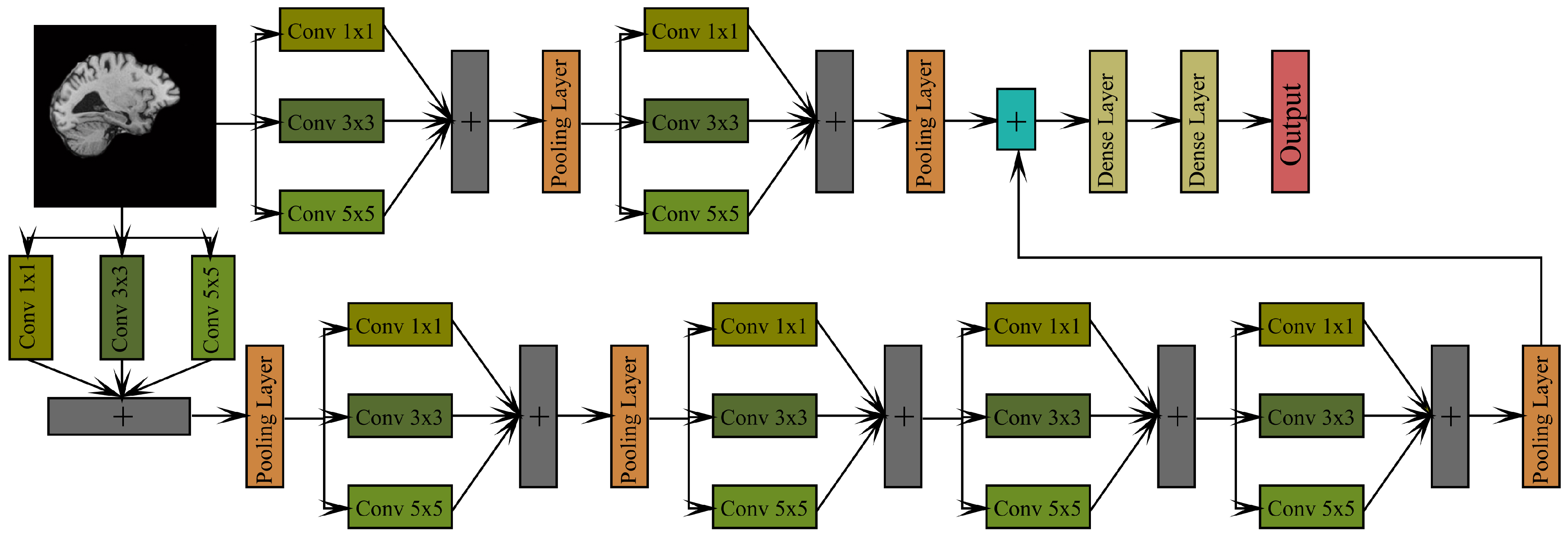
• The main aim of this work is to develop a light weighted hybrid model that can perform faster and better. We combined LeNet and AlexNet in parallel and proposed a new hybrid DNN architecture.
• Different convolutional kernel sizes may help a network to learn more crucial aspects, and mixing several features can improve feature representations [39]. Hence, in the proposed hybrid model, we replaced all the traditional large convolutional filters with a set of three small filters ($1\times 1,3\times 3$, and $5\times 5$).
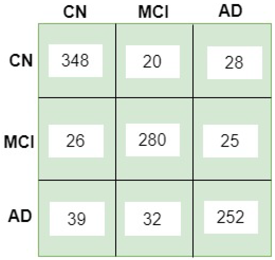
• Better feature extraction improves the model’s performance, and the model’s average performance improved to 93.58%. Mathematically, it is shown that the proposed hybrid model retrieved much fewer convolutional parameters (even significantly fewer than the regular AlexNet model), making it a computationally faster model.
• In comparison to all other deployed models, as well as the discussed state of the art, it is observed that the proposed hybrid model achieved the most convincing performance.

The organization of the paper is as follows: (a) In Section 2, we discussed some of the recently published related state of the art. (b) In Section 3, we discussed and evaluated the performance of some existing DNN models for AD classification. (c) In Section 4, the proposed hybrid model is discussed and evaluated using the same data set. (d) In Section 5, Results, a discussion is given. (e) In Section 6, we concluded the paper along with a discussion about some future scopes of work.

2. Related Study

In the diagnosis of Alzheimer’s disease, ANN methods are becoming increasingly popular. One of the key reasons for its popularity is the ability to learn about the best features from the surroundings to improve its forecasting accuracy over time [40]. Some of the recently published state-of-the-art works are discussed in this section.

A ResNet-based model for brain shrinkage identification that further helps in AD classification is proposed in ref. [41]. Initially, a DNN of residual self-attention is developed to increase the classification efficiency by integrating local–global along with spatial features from brain scans. For enhancing the intelligible characteristics, a gradient-based localisation class activation mapping (g-LCAM) based intelligibility procedure is developed. Finally, the authors propose an automatic classification approach which is based on the sub-sequential training. The proposed 3D model is inspired from the original ResNet model. In order to achieve the most convincing results, the 3D g-LCAM is used in the model. The proposed model can classify AD/CN, and progressive MCI (pMCI)/ stable MCI (sMCI).

In a related work, a new broad learning system (BroLeS) based model for the categorization of AD is proposed in ref. [42]. The diagnosis method employs brain MRIs and leverages BroLeS and its convolutional advances to categorize several stages of Alzheimer’s disease. The computational anatomy toolbox (CAT-12) is used to perform various pre-processing tasks. A new model is developed, known as the convolution feature-based cascade of enhancement nodes BroLeS (CCEBroLeS) based on processed data that aid in merging BroLeS variants. As a result, a new version is offered that incorporates both the CCEBroLeS and the BroLeS. For feature extraction, a multi-layer CNN is utilised. The model is based on the well-known VGG model.

An artificial neural network-based AD diagnosing model that can also predict the progression of the disease is proposed in ref. [43]. A 3d multi-information generative adversarial network (MulGAN) is used in order to determine brain changes as age progresses. A DenseNet-based model is built to classify the disease that fundamentally optimises the localized degradation of brain to predict Alzheimer stages. The model incorporates a variety of factors, including age, gender, and so on. The Voxel-based morphometry (VoBM) toolkit is used in pre-processing to conduct skull removal and the splitting of brain images into 3 sections (grey matter, white matter, and cerebrospinal fluid). The presented method can differentiate various phases of cognition, such as MCI vs. AD, MCI vs. CN, pMCI vs. sMCI, and so on. The model was also tested as a multiclass classifier and came out with a positive result.

Taking brain atrophy as an important bio-marker, a new AD classification approach is introduced in ref. [44]. The model can be used for both atrophy identification and classification. For determining the most discriminatory regions, a cluster-based CNN is designed. Crucial characteristics are retrieved from the detected locations and utilised for training the model. Information from regional brain MRI slices is also used in the training of the model. A cell-based anatomy with each of the axially aligned images is created to obtain the approximated positions for extracting the features. A composite loss function is used to improve the results.

A CNN-based AD diagnostic system is proposed in ref. [45]. A CNN model is designed that incorporates the most relevant characteristics of the hippocampal lobes utilizing T1-MR and FDG-PET data. No splitting procedures are carried out. All image data are converted as the identical spatial space to prepare data in training and testing. Rigid normalization is used to ensure that the cells from same brain areas from both sources are the same. The concept of original VGG model is taken as reference while building the proposed model. CN vs. AD, CN vs. pMCI, and sMCI vs. pMCI individuals are classified using the proposed model.

A novel DNN model that can classify AD from DT images is proposed in ref. [46]. Pre-processing, such as normalisation, RoI separation, etc., is performed utilising the statistical parametric mapping software. After performing the segmentation, a separate volumetric measurement is performed for GM and WM. The proposed model is the combination of an input, convolution, batch-normalization, activation, pooling, dense, and the final classifying layer. Five-cross validation enhanced the training/testing performance of the model.

An AD classifier is developed using a fusion of CNN with the recurrent neural networks in a research work [47]. All 3D brain images are processed into a series of 2D slices. A mixture of convolutional and recurrent neural networks is used to fit the classifier appropriately on intra–inter characteristics. Slice-wise characteristics are adopted using CNNs, and multi-characteristics are adopted using RNNs’ gated recurrent unit.

A DenseNet-based strategy for AD detection is proposed in ref. [48]. Some of the effective slices are used for further analysis from 3D MR data. In the proposed model, the concept of the DenseNet’s Bottleneck is used. A channel factor is also used that takes into account three specific channels (RGB) from monocular MRIs. The M3d-Cam toolkit is combined with a guided gradient weighted class activation mapping (Grad-CAM) technique to improve imaging feature extraction. The procedure is known as attention mapping, and it aids in the discovery of undesired characteristics. All undesirable pixels are therefore eliminated using the proper processing methods.

An artificial neural network model for AD diagnosing using the brain MR data is proposed in the research work of [49]. The 3D Slicer toolkit is used to separate the hippocampal lobes from brain data. The surface of voxels is then processed using an uniformity rectifying analysis based on Local-Entropy-Minimization-bi cubic Spline. Eventually, the diagnoses are carried out using a CNN-based predictor. The input layer, convolutional layers, pooling layers, flatten layers, fully connected layers, and output class label make up the proposed CNN.

By using the concept of extreme learning, a novel CNN model for AD classification is proposed in ref. [50]. Cognitive control networks are classified using two distinct networks. Additionally, the concept of an enhanced extreme learning machine is also used.

Employing extreme learning, the model is trained on elements of deep regional connectivity. Extreme learning is also used to assist the network in learning more about characteristics in the area. The Pearson correlation (PC) coefficient is used to construct the brain network. The suggested DNN is made up of convolutional layers, the ReLu activation function, pooling layers, fully linked layers, and decision layers.

For staging the AD spectrum, a RoI-CNN based classifier is proposed in a research article [51]. Patches of three orthogonal views of selected RoIs from cerebral regions are used to train a CNN model. From the brain images, the hippocampus, amygdala and insulae regions are chosen as RoIs. Softmax activation function is used to predict the probability of the AD stages. The Gwangju Alzheimer and Related Dementia (GARD) data set is used. RoI-basd data are used in a CNN for binary classifications. Then classifiers are grouped together for staging the AD. A permutation test is performed to choose the specific 3 pairs of ROIs from 101 different ROIs in the data set.

From the discussion about various recently published state-of-the-art works, it is observed that the majority of the papers did not give a high priority to computational time. Moreover, the highest performance is reported as 90%. So to enhance both the computational and classification performance results, we propose a hybrid approach that generates fewer parameters to make it a light-weight model (discussed in Section 4).

3. Experimental Analysis of Different DNN Models

3.1. Data and Tools

T1-weighted, MPRAGE MRI data are acquired from the online data set ADNI [52]. During the acquisition of data, a total of 150 subjects (CN: 50, MCI: 50, AD: 50) are considered.

Throughout ageing, the thickness and biological structures of the human brain changes [53,54]. Our earlier studies [55,56] showed that the hippocampal size as well as the volume of grey matter (GM) varies with the individual’s ageing. It is observed that the average hippocampal and GM size/volume is higher in participants in a certain category (CN, MCI, or AD) aged 60–69 years than any other ages (70+ years). Similarly, individuals in their 70s and 80s have greater hippocampal/GM areas than those in their 80s and 90s. As a consequence, all training and testing data are separated into multiple subgroups depending on patient age (60–69/70–79/80+ years) for better evaluation of the algorithms.

The actual number of training images was 5000. We used the Data-Gen process to generate a large amount of training data with several variables, such as rotation, mirror reflection, and so on. The total number of images surpassed 11,000.

Table 1. Data distributions.

Classes	Subjects	Age (Years)	Training Images	Testing Images	Total No. Images
CN	50	60–69	900	350	3750
		70–79	900	350
		80+	900	350
MCI	50	60–69	900	350	3750
		70–79	900	350
		80+	900	350
AD	50	60–69	900	350	3750
		70–79	900	350
		80+	900	350
Total	150	8100		3150	11,250

shows how all of the data are organized.

3.2. Experimental Setup

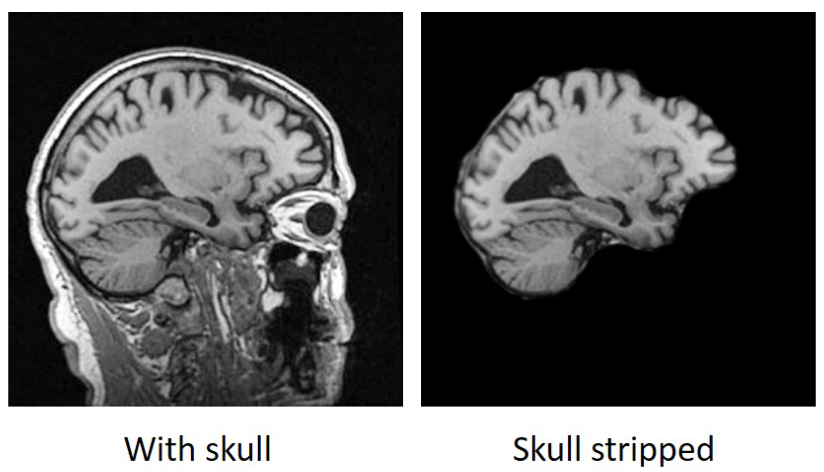
The CPU used in this work is configured with (a) 12 GB of RAM (b) 500 GB of SSD storage, (c) 2 GB graphics, and (d) i7 processor. For implementations, we used the Python 3.0 toolkit. We employed the “softmax” activation function, the “StochasticGradientDescent (SGD)” optimizer, and the “SparseCategoricalCrossEntropy (SCCE)” loss function for all of the models. The data are split into 32 batches and trained across 40 epochs.

3.3. Pre-Processing

With the help of a radiologist from the North Eastern Indira Gandhi Regional Institute of Health and Medical Sciences (NEIGRIHMS), we performed a pre-processing step for selecting an appropriate slice from the 3D images. By utilizing 3D slicer software, we selected a slice of the image where the hippocampus region can be visualised properly. The reason behind taking the hippocampus as a region of visual interest is that, in AD, the hippocampus is the primarily affected region in the brain. After obtaining the 2D images, we applied the skull-stripping operation.

All data acquired from the data set ADNI are not skull-free. In our study, the skull is unnecessary; hence, we performed the skull-stripping operation before training the models. Five frequently utilized segmentation strategies, including region-growing, region splitting–merging, K-means clustering, histogram-based thresholding, and the fuzzy c means method, are examined to separate the skulls more precisely [57]. As shown in

Table 2. Performance analysis of various skull-stripping approaches.

Algorithm	Accuracy	Sensitivity
Region growing	0.62	0.68
Histogram based	0.85	0.90
Fuzzy C means	0.53	0.77
K-Means	0.64	0.75
Region Splitting and Merging	0.61	0.74

, it is observed that the histogram-based thresholding technique can deliver a reasonable outcome [57]. As a result, a histogram-based technique is used to remove the skull. Figure 2 shows an example of an input and the corresponding output result (skull stripping).

3.4. Discussion about the Implemented DNN Models

Below is a brief overview of all the models that have been implemented.

3.4.1. LeNet

In 1989, Yann LeCun presented one of the most simplest and effective DNN architectures with only 7 layers [30]. The arrangement of the layers can be summarized after the input as (1) conv layer, (2) pooling layer, (3) conv layer, (4) pooling layer, (5) fully connected layer, (6) fully connected layer, and (7) the output layer. In CNN, the convolution layer has the responsibility for extracting the important features from the input data. By learning attributes with smaller sections of input data, convolution maintains the correlation among pixels. It is a computational process with two variables: image matrix as well as a filter/kernel. A sample convolutional operation can be presented as Equation (1).

$$C_{xy}=C(m,n)=b+{(A·B)}_{mn}=b+\sum _x\sum _y{A}_{m-x,n-y}·B_{x,y}$$

(1)

In Equation (1), ‘C’ stands for convolution, ‘A’ stands for input, and ‘B’ stands for kernel function, and ‘b’ is bias value. The matrices’ rows and columns are denoted by ‘x’ and ‘y’.

The pooling operation implies rolling a 2D kernel across each channel of the feature space and aggregating the features that fall inside the filter’s coverage zone. Data maps’ dimensionalities are reduced by using pooling layers. As a result, the set of variables to train as well as the cost of processing in the networks are both reduced. There are three types of pooling layers used by different DNN models, which are max pooling, average pooling, and global pooling.

3.4.2. AlexNet

AlexNet was first introduced by Krizhevesky in 2012 [58]. AlexNet, which uses an 8-layer network, blew away the competition in the ILSVRC 2012 [59]. AlexNet and LeNet have nearly identical design ideas, yet they also have substantial variances. Firstly, AlexNet is substantially larger than LeNet, which is comparably smaller. AlexNet has 8 layers, including 5 convolutional layers and 2 dense layers, followed by an output layer. Secondly, AlexNet adopts the ReLu activation function instead of sigmoid. This model demonstrates that learning-based features can outperform manually designed features, shattering the old paradigm in machine vision.

3.4.3. VGG-16 and VGG-19

The VGG-16 architecture, often known as VGGNet-16, is a CNN model introduced by A. Zisserman and K. Simonyan of Oxford university in 2014 [32]. VGG-16, which has a total of 16 deep layers, was designed for the Visual Geometry Group (VGG) Lab. In ILSVRC-2014, VGG 16 won the competition for localisation, finishing 2nd for classifications [60]. VGG-16 consists of 13 convolutional, 5 pooling, and a set of dense layers. VGG-19 follows a similar architecture as VGG-16 with a sum of 47 layers (having 19 deep layers) [61].

3.4.4. Inception—V1 and V2 and V3

Although architectures of deep CNN, such as VGG-16 and VGG-19, can convincingly perform classification tasks, but they sacrifice computation time [62]. Furthermore, over-fitting difficulties have an impact on such networks, and it is difficult to propagate gradient modifications across the entire network. Lin et al. developed the notion of the inception module in 2014 to address these challenges [33]. The main goal of the inception block is to estimate an ideal local sparse organization. It lets us employ many sorts of filter sizes in a single image block, rather than being limited to a single filter size, and finally the combination of all will be forwarded to the next layer. Szegedy et al. then developed the architecture of Inception-V1 (which is also known as GoogleNet) by borrowing the concept of the inception module [63]. Inception-V1 was chosen the winner of the ILSVRC 2014. Including several inception modules, this model is designed with a total of 22 layers and in each module, a set of $1\times 1$, $3\times 3$, and $5\times 5$ filters is used.

Although the achievement of Inception-V1 is adequate, the topology has a flaw. The utilization of larger filters, such as $5\times 5$, can cause the input parameters to diminish by a large factor, possibly resulting in the loss of vital information [64]. To address this problem, the Inception-V2 framework is created, in which each of the $5\times 5$ convolutions is modified with 2 $3\times 3$ [65]. Additional modification to this approach is the replacement of the $n\times n$ computation with $n\times 1$ and $1\times n$, which improves the method to be operationally quicker.

Inception V3 is introduced by upgrading and adding some new concepts, including label filtering, uses of $7\times 7$ filters, use of the RMSprop estimator, and so on [65]. Inception-V3 came in second place in the ILSVRC contest in 2015 [66].

3.4.5. ResNet-50

Although deep models, such as Inception, produce impressive findings, as the network grows deeper, it becomes saturated and loses accuracy quickly [34,67]. The notion of a residual block is developed to overcome the problem. The fundamental idea is to create a bridging that enables to bypass 1 or even more layers. The concept of residual blocks worked successfully, as ResNet won the ILSVRC 2015 championship [68]. The ResNet-50 can be divided into five blocks, each block owning a collection of convolution and residual blocks.

3.4.6. MobileNet-V1

MobileNet is well known for its use in lightweight apps [69]. The notion of depth-wise convolutions is applied in this framework, which aids in the reduction of less significant parameters [35]. Convolutional function is divided into two parts: initially, a depth-wise convolutional layer which is used to filter the input, and then an $1\times 1$ (also known as point-wise convolution) convolutional layer merges the processed information to form new features.

3.4.7. EfficientNet-B0

Tan et al. introduced a novel prototype scaling strategy in 2019 that is built on a basic compounded coefficient that helps in scaling up the networks in a more ordered manner [36]. Traditionally, dimension scaling is performed by taking the width/depth/resolution as a factor, but EfficientNet uses a vector of scaling coefficients [70]. This technique is also called compound scaling (CS). If, for a particular input channel, the depth, width, and resolution are given by $m=a^{\varphi }$, $n=b^{\varphi }$, and $o=c^{\varphi }$ correspondingly, where $\varphi$ represents the compound coefficient, then the mathematical expression of CS can be defined as (2):

$$CS=a·b^2·c^2\approx 2,a\ge 1,b\ge 1,c\ge 1$$

(2)

3.4.8. Xception

Google team designed this new CNN architecture based on the Inception network topologies with the introduction of a new idea termed depth-wise separable convolution [37]. This new idea of the convolution technique is simply a revised form of the depth-wise convolution. The operation starts with a $1\times 1$ convolution and then proceeds to channel-wise spatial convolutional procedures. The non-linearity of the inception model is removed in Xception by applying the depth-wise separable convolution.

3.4.9. DenseNet-121

In deeper models, the communication route from the origin to destination, as well as the gradient that traverses in the opposite direction, can become so long that certain information gets lost even before it achieves the given target [71]. DenseNet changed the way the layers communicate with one another. All layers in the network are intrinsically linked, and the idea of feature reuse is used to lower the overall amount of parameters. Another difficulty with DNN models is that they follow knowledge transfer and also gradients during learning. To address this problem, DenseNets provides all layers with the ability to directly acquire gradients by matching loss functions [38].

We evaluated several of the most common parameters, including accuracy, precision, recall, and F1-score, to evaluate performance. The aggregate of all of these key metrics is computed. The overall evaluation is presented in

Table 3. Performance comparison of different DNN models for AD classification.

Models	Performance (Average)	p-Value	Average Time Required per Epoch
LeNet	0.8025	0.025	68 s
AlexNet	0.7150	0.033	79 s
VGG-16	0.7900	0.027	142 s
VGG-19	0.8525	0.041	248 s
Inception-V1	0.8280	0.035	228 s
Inception-V2	0.8275	0.042	188 s
Inception-V3	0.8360	0.031	212 s
ResNet-50	0.7125	0.022	552 s
MobileNet-V1	0.8640	0.192	532 s
EfficientNet-B0	0.7360	0.022	0842 s
Xception	0.86	0.027	774 s
DenseNet-121	0.8655	0.018	812 s

.

From Table 3, it can be noticed that the highest average performance is achieved by the DenseNet-121 model. However, the model compromises with the execution complexity. LeNet and AlexNet, on the other hand, have the fastest execution times because of their simple and effective architectures. Our major goal is to design an effective architecture that can perform better and faster. We propose a hybrid architecture where LeNet and AlexNet combined together. A detailed discussion of the architecture is given in Section 4.

4. Proposed Model for AD Classification

The ensemble of different DL models is a popular way to enhance classification performance results. Effective examples of ensembles of different ML models for automatic sleep–arousal detection, attention classification, etc., can be observed in refs. [72,73]. By taking the original LeNet and AlexNet architectures as a reference, we propose a new model, where all the layers of both models are combined parallelly. Apart from that, since our region of interest is the brain, which is not very large, and since different convolutional kernel sizes help a model to learn better [39], we replaced the large convolutional filters from the original architectures with a set of three small parallel filters ($1\times 1,3\times 3,5\times 5$). The architecture of the proposed model is presented in Figure 3.

In Figure 3, the symbol ‘+’ represents the concatenation of different layers. The average performance of the model is presented in

Table 4. Performance evaluation table of the proposed hybrid model.

Model	Classes	Age (Years)	Accuracy	Precision	Recall	F1 Score	Average Performance	Average Time per Epoch
Proposed Hybrid Model	CN/MCI	60–69	0.95	0.93	0.95	0.94	0.9358	72 s
		70–79	0.93	0.94	0.95	0.94
		80+	0.95	0.94	0.92	0.94
	MCI/AD	60–69	0.93	0.93	0.92	0.96
		70–79	0.96	0.93	0.93	0.96
		80+	0.92	0.92	0.95	0.92
	CN/AD	60–69	0.96	0.96	0.94	0.93
		70–79	0.92	0.93	0.92	0.93
		80+	0.91	0.92	0.93	0.93

.

One of the primary motivations for substituting normal convolution layers is to accelerate up the model by extracting fewer but more diverse parameters. Instead of employing a large number of kernels with the same enormous filter size, we broke it down into three separate filter sizes. This phase not only assisted us in obtaining multiple features, but it also resulted in fewer parameters, allowing the model to run more efficiently. The mathematical advantages of adopting a set of small kernel sized convolution layers are addressed in the next paragraph.

Considering no padding and 1 stride, if we use ‘M’ number of ’$K_h\times K_w$’ kernels in a convolution layer followed by a prior layer with ‘N’ number of kernels, the total number of parameters ‘P’ generated in the current convolution layer can be represented by Equation (3):

$$P=((K_h\times K_w\times N)+1)\times M$$

(3)

where 1 is added as the bias term in each filter. In the original LeNet architecture, it has a total of two convolution layers with $6,5\times 5$, and $16,5\times 5$, filters. If the input dimension is $256\times 256\times 3$, the number of parameters generated by each of the convolution layers can be calculated as follows:

• No. of parameters generated by first convolution layer = $\left(\right(5\times 5\times 3)+1)\times 6)=456$.
• No. of parameters generated by second convolution layer = $\left(\right(5\times 5\times 6)+1)\times 16)=2416$.
• Total parameters generated in LeNet by the two convolution layers = 2872.

Similarly, the parameters generated by all the five convolution layers in standard AlexNet architecture with ($96,11\times 11$), ($256,5\times 5$), ($384,3\times 3$), ($384,3\times 3$), and ($256,3\times 3$) filters can be calculated as follows:

• No. of parameters generated by first convolution layer = $\left(\right(11\times 11\times 3)+1)\times 96)=34,944$.
• No. of parameters generated by second convolution layer = $\left(\right(5\times 5\times 96)+1)\times 256)=614,656$.
• No. of parameters generated by third convolution layer = $\left(\right(3\times 3\times 256)+1)\times 384)=885,120$.
• No. of parameters generated by fourth convolution layer = $\left(\right(3\times 3\times 384)+1)\times 384)=1,327,488$.
• No. of parameters generated by fifth convolution layer = $\left(\right(3\times 3\times 384)+1)\times 256)=884,992$.
• Total parameters generated in LeNet by the two convolution layers = 3,747,200.

If we add the original LeNet and AlexNet architectures together, then we will get a total number of 3,750,072 convolutional numbers. Since the number of parameters is huge, it will make the hybrid model slower in execution. Hence, we introduced the concept of multiple small sized kernels in the original convolution layers to gain a variety of features that can also reduce the total number of parameters significantly. In the modified LeNet architecture, we divided the total number of kernels in three parts in each of the convolution layers. In the modified convolution layers of LeNet, we have $\left[\right(2,1\times 1),(2,3\times 3),(2,5\times 5\left)\right]$, and $\left[\right(6,1\times 1),(6,3\times 3),(6,5\times 5\left)\right]$, filters. The number of parameters generated by each of the modified convolution layers can be calculated as follows:

• No. of parameters generated by first convolution layer = $\left[\right((1\times 1\times 3)+1)\times 2)+\left(\right(3\times 3\times 3)+1\times 2)+\left(\right(5\times 5\times 3)+1\times 2)]=214$.
• No. of parameters generated by second convolution layer = $\left[\right((1\times 1\times 2)+1)\times 6)+\left(\right(3\times 3\times 2)+1\times 6)+\left(\right(5\times 5\times 2)+1\times 6)]=438$.
• Total parameters generated in LeNet by the two convolution layers = 652.

Similarly, the parameters generated by all the five convolution layers in standard AlexNet architecture with $\left[\right(32,1\times 1),(32,3\times 3),(32,5\times 5\left)\right]$, $\left[\right(86,1\times 1),(86,3\times 3),(86,5\times 5\left)\right]$, $\left[\right(128,1\times 1),(128,3\times 3),(128,5\times 5\left)\right]$, and $\left[\right(128,1\times 1),(128,3\times 3),(128,5\times 5\left)\right]$, and $\left[\right(86,1\times 1),(86,3\times 3),(86,5\times 5\left)\right]$ filters can be calculated as follows:

• No. of parameters generated by first convolution layer = $\left[\right((1\times 1\times 3)+1)\times 32)+\left(\right(3\times 3\times 3)+1\times 32)+\left(\right(5\times 5\times 3)+1\times 32)]=3776$.
• No. of parameters generated by second convolution layer = $\left[\right((1\times 1\times 32)+1)\times 86)+\left(\right(3\times 3\times 32)+1\times 86)+\left(\right(5\times 5\times 32)+1\times 86)]=96,578$.
• No. of parameters generated by third convolution layer = $\left[\right((1\times 1\times 86)+1)\times 128)+\left(\right(3\times 3\times 86)+1\times 128)+\left(\right(5\times 5\times 86)+1\times 128)]=385,664$.
• No. of parameters generated by fourth convolution layer = $\left[\right((1\times 1\times 128)+1)\times 128)+\left(\right(3\times 3\times 128)+1\times 128)+\left(\right(5\times 5\times 128)+1\times 128)]=573,824$.
• No. of parameters generated by fifth convolution layer = $\left[\right((1\times 1\times 128)+1)\times 86)+\left(\right(3\times 3\times 128)+1\times 86)+\left(\right(5\times 5\times 128)+1\times 86)]=385,538$.
• Total parameters generated in LeNet by the two convolution layers = 1,445,380.

The proposed hybrid model (modified LeNet + modified AlexNet) generates 1,446,032 convolutional parameters, which is 2,304,040 lesser than the original architecture. It can be clearly observe that the proposed model generates significantly fewer convolutional parameters, resulting in a model that is lighter in weight and faster.

It is also worth noting that the number of convolutional parameters in the hybrid model is even much lower than the original AlexNet (parameters difference is 2,301,168), which makes the hybrid model even faster than the original AlexNet model. The hybrid model not only outperforms all other models in terms of execution time, but it also has a better ability to classify AD. In Table 4, the average performance of the proposed hybrid model is presented.

All the performances evaluated in this work are examined over test images. The performance evaluation metrics used in this work are accuracy, precision, recall, and F1 score. The percentage of correct forecasts (true positive + true negative) among all guesses is known as accuracy. The number of correctly predicted positive outcomes (true positive) is measured by precision. The percentage of positive cases the classifier accurately predicted out of all the positive instances in the data is known as recall. The F1-score is a measurement that combines recall and precision. Overall, it is referred to as the mean of the two.

From Table 4, it can be observed that the average performance of the proposed hybrid model, which is around 93.58%, is the maximum among all the implemented models. Moreover, the average time required per epoch in the proposed model is lower than most of the discussed models.

The proposed model is also tested for multi-class classification (CN vs. MCI vs. A) using 5-fold cross validation. The dataset is split into 5 folds, where examples are assigned randomly to each fold. For each one of the ith runs (where i = 1 to 5), assign examples in the ith fold for testing with the remaining examples in the other folds for training. Then, perform predictions on the ith testing fold. The performance observed is presented in

Table 5. Multi-class performance evaluation table of the improved LeNet model.

Model	Age (Years)	Accuracy	Precision	Recall	F1 Score
Proposed Hybrid model	60–69	0.88	0.92	0.90	0.91
	70–79	0.83	0.88	0.89	0.89
	80+	0.83	0.85	0.84	0.85

.

The best-performing confusion matrix for multi-class classification is shown in Figure 4.

From Table 5, the standard deviation ($\sigma$) is determined as Equation (4):

$$\sigma =\sqrt{\frac{1}{T}\sum _{i=1}^T{(x_i-\mu )}^2}$$

(4)

In Equation (4), T is the population size (3). Mean Performance = 0.87; Sum of difference (s) = $(x_i-\mu )$ =0.002; Variance (${\sigma }^2$) = s/T = 0.0027/3 = 0.001; Deviation ($\sigma$) = $\sqrt{0.0013}$ = 0.032.

5. Results and Discussion

Some of the most commonly used DL models are implemented for AD classification using the same dataset and the same experimental setup. As presented in Table 3, the average performance results of all implemented models are observed. It is observed from Table 3 that LeNet and AlexNet are computationally faster (68 s/epoch, and 79 s/epoch) than all other implemented models. The idea of this work is to design a hybrid approach that can classify AD efficiently with less computational time. Hence, we combined LeNet and AlexNet with certain modifications.

After combining LeNet and AlexNet with certain modifications, the hybrid model is tested for binary class classifications. As presented in Table 4, we observed the performance with some widely used evaluation matrices, such as accuracy, precision, recall, and F1 score. According to the average value shown in Table 4, it is observed that the hybrid model can outperform all implemented DL models (except the original LeNet) in terms of performance (93.58%) and computational time (72 s/epoch).

The same hybrid model is also tested for multi-class classifications. For better performance analysis, we used a 5-fold cross-validation approach. The multi-class classification performance is presented in Table 5. Table 5 shows that the proposed hybrid approach can be utilized effectively for multi-class categorization as well.

As some of the recently published related state-of-the-art works are discussed, we made a performance comparison of all the discussed state-of-the-art work with the proposed approach (in the referred similar works, authors mentioned the performance of their models). It is observed from

Table 6. Performance comparison amongst the discussed AD classification approaches.

Sl No.	Authors	Dataset	Average Performance
01	Zhang et al. [41]	ADNI	86.34%
02	Han et al. [42]	ADNI	89.6%
03	Zhao et al. [43]	ADNI	77.39%
04	Lian et al. [44]	ADNI	82.63%
05	Huang et al. [45]	ADNI	84.82%
06	Marzban et al. [46]	ADNI	86.15%
07	Liu et al. [47]	ADNI	89.6%
08	Rojas et al. [48]	ADNI	88.6%
09	Choi et al. [49]	ADNI	85.34%
10	Xin Bi, et al. [50]	ADNI	83.27
11	Ahmed, et al. [51]	Gwangju Alzheimer Research Data (GARD)	90%
Proposed Hybrid model		ADNI	93.58%

that the proposed hybrid approach can outperform all the discussed state-of-the-art works convincingly.

As compared in Table 3 and Table 6, it can be observed that amongst all the discussed models and state-of-arts, the proposed hybrid approach can classify AD more convincingly.

From Table 6, it can be observed that, amongst all the implemented models, EfficientNet requires the maximum time for execution. The proposed hybrid approach requires approximately 72 s per epoch, which is the minimum among all implemented models (except the original LeNet).

6. Conclusions and Future Work

In this experimental work, we took 12 of the most commonly used DNN models for implementation. We tested the models using the same data which were acquired from the online database ADNI. There are three classes considered for classification (CN, MCI, and AD). All data were further distributed separately for different age groups. From the implementation results, it was observed that the DenseNet performed most convincingly but took much computational time. Although the LeNet and AlexNet performance results are not as good as that of DenseNet, their simple and effective architecture allows them to run significantly faster. Given the importance of computing time, we presented a new hybrid DNN model in which we integrated LeNet and AlexNet in parallel. However, the proposed model would take longer time to implement due to its complicated architecture and high convolutional operations. We replaced all of the typical convolution layers with a series of three small parallel convolution layers having $1\times 1,3\times 3$, and $5\times 5$ filters to fix this issue, which also allowed the model to extract more significant features. Mathematically, the proposed hybrid model extracted much fewer convolutional parameters than all of the other models (except LeNet) presented, revealing that it is one of the most light-weight models. We discussed some of the recently published state-of-the-art work to compare our work. From the experimental evaluation, it was observed that the average performance of the proposed hybrid model not only outperformed all the implemented models but also all the discussed state-of-the-art works. The proposed model’s average performance is approximately 93.58%, and training takes around 72 s per epoch, which is faster than all the discussed models (except the original LeNet model).

This work demonstrates that large convolutional filters are not necessarily required to extract features for image classification using DNN. More relevant features can be extracted by combining more than two small-sized kernels, which results in significantly fewer parameters and reduces computing time.

Although the proposed DNN model can classify AD convincingly, the model can be further improved in future work. The performance of the model may be further improved by adopting advanced DNN concepts, such as the Dense-block notion, that can help the model with gradient losses. For better feature extraction, GA based approach may be utilized in the proposed model. Since lower-intensity valued pixels may also contain important information, a hybrid pooling layer (Min + Max pooling) may help the model in adopting more relevant features. In this work, only one data-set ADNI is used. In the future, more data from different databases can be acquired to compare and improve the results. The performance of the model can be compared with some more advanced DNN-based approaches. Only MRI is used in this work; in the future, more modalities of images, such as CT images, PET, etc., can be acquired and tested in the model.

References

1. Alzheimer’s Association. 2018 Alzheimer’s disease facts and figures. Alzheimer’s Dement. 2018, 14, 367–429. [Google Scholar] [CrossRef]
2. Korolev, I.O. Alzheimer’s disease: A clinical and basic science review. Med. Stud. Res. J. 2014, 4, 24–33. [Google Scholar]
3. Donev, R.; Kolev, M.; Millet, B.; Thome, J. Neuronal death in Alzheimer’s disease and therapeutic opportunities. J. Cell. Mol. Med. 2009, 13, 4329–4348. [Google Scholar] [CrossRef] [PubMed] [Green Version]
4. Moon, S.W.; Lee, B.; Choi, Y.C. Changes in the hippocampal volume and shape in early-onset mild cognitive impairment. Psychiatry Investig. 2018, 15, 531. [Google Scholar] [CrossRef] [Green Version]
5. Barnes, J.; Whitwell, J.L.; Frost, C.; Josephs, K.A.; Rossor, M.; Fox, N.C. Measurements of the amygdala and hippocampus in pathologically confirmed Alzheimer disease and frontotemporal lobar degeneration. Arch. Neurol. 2006, 63, 1434–1439. [Google Scholar] [CrossRef] [Green Version]
6. Hazarika, R.A.; Maji, A.K.; Sur, S.N.; Paul, B.S.; Kandar, D. A Survey on Classification Algorithms of Brain Images in Alzheimer’s Disease Based on Feature Extraction Techniques. IEEE Access 2021, 9, 58503–58536. [Google Scholar] [CrossRef]
7. NIH. Alzheimer’s Disease: A Clinical and Basic Science Review. Available online: https://www.nia.nih.gov/health/alzheimers-disease-fact-sheet (accessed on 13 July 2020).
8. Alzheimer’s Association. Alzheimer’s Disease Fact Sheet. Available online: https://www.alz.org/in/dementia-alzheimers-en.asp#diagnosis (accessed on 13 July 2020).
9. Varatharajah, Y.; Ramanan, V.K.; Iyer, R.; Vemuri, P. Predicting short-term MCI-to-AD progression using imaging, CSF, genetic factors, cognitive resilience, and demographics. Sci. Rep. 2019, 9, 1–15. [Google Scholar] [CrossRef] [Green Version]
10. National Institute on Aging(NIH). What Is Mild Cognitive Impairment? Available online: https://www.nia.nih.gov/health/what-mild-cognitive-impairment (accessed on 23 June 2021).
11. Burns, A.; Iliffe, S. Clinical review: Alzheimer’s disease. Br. Med. J. 2009, 338, b158–b163. [Google Scholar] [CrossRef] [Green Version]
12. Mayo Clinic Staff. Learn How Alzheimer’s Is Diagnosed. 2019. Available online: https://www.mayoclinic.org/diseases-conditions/alzheimers-disease/in-depth/alzheimers/art-20048075 (accessed on 23 June 2021).
13. Huff, F.J.; Boller, F.; Lucchelli, F.; Querriera, R.; Beyer, J.; Belle, S. The neurologic examination in patients with probable Alzheimer’s disease. Arch. Neurol. 1987, 44, 929–932. [Google Scholar] [CrossRef]
14. Arevalo-Rodriguez, I.; Smailagic, N.; i Figuls, M.R.; Ciapponi, A.; Sanchez-Perez, E.; Giannakou, A.; Pedraza, O.L.; Cosp, X.B.; Cullum, S. Mini-Mental State Examination (MMSE) for the detection of Alzheimer’s disease and other dementias in people with mild cognitive impairment (MCI). Cochrane Database Syst. Rev. 2015, 23, 107–120. [Google Scholar] [CrossRef]
15. Cummings, J.L.; Ross, W.; Absher, J.; Gornbein, J.; Hadjiaghai, L. Depressive symptoms in Alzheimer disease: Assessment and determinants. Alzheimer Dis. Assoc. Disord. 1995, 9, 87–93. [Google Scholar] [CrossRef] [PubMed]
16. Symms, M.; Jäger, H.; Schmierer, K.; Yousry, T. A review of structural magnetic resonance neuroimaging. J. Neurol. Neurosurg. Psychiatry 2004, 75, 1235–1244. [Google Scholar] [CrossRef] [PubMed]
17. Ijaz, M.F.; Attique, M.; Son, Y. Data-driven cervical cancer prediction model with outlier detection and over-sampling methods. Sensors 2020, 20, 2809. [Google Scholar] [CrossRef]
18. Ledig, C.; Schuh, A.; Guerrero, R.; Heckemann, R.A.; Rueckert, D. Structural brain imaging in Alzheimer’s disease and mild cognitive impairment: Biomarker analysis and shared morphometry database. Sci. Rep. 2018, 8, 1–16. [Google Scholar] [CrossRef] [Green Version]
19. Fung, Y.R.; Guan, Z.; Kumar, R.; Wu, J.Y.; Fiterau, M. Alzheimer’s disease brain mri classification: Challenges and insights. arXiv 2019, arXiv:1906.04231. [Google Scholar]
20. Lundervold, A.S.; Lundervold, A. An overview of deep learning in medical imaging focusing on MRI. Z. Med. Phys. 2019, 29, 102–127. [Google Scholar] [CrossRef]
21. Wang, S.C. Artificial neural network. In Interdisciplinary Computing in JAVA Programming; Springer: Berlin/Heidelberg, Germany, 2003; pp. 81–100. [Google Scholar]
22. Pagel, J.F.; Kirshtein, P. Machine Dreaming and Consciousness; Academic Press: Cambridge, MA, USA, 2017. [Google Scholar]
23. Raghavan, V.V.; Gudivada, V.N.; Govindaraju, V.; Rao, C.R. Cognitive Computing: Theory and Applications; Elsevier: Amsterdam, The Netherlands, 2016. [Google Scholar]
24. Esteva, A.; Robicquet, A.; Ramsundar, B.; Kuleshov, V.; DePristo, M.; Chou, K.; Cui, C.; Corrado, G.; Thrun, S.; Dean, J. A guide to deep learning in healthcare. Nat. Med. 2019, 25, 24–29. [Google Scholar] [CrossRef] [PubMed]
25. Khasawneh, N.; Fraiwan, M.; Fraiwan, L. Detection of K-complexes in EEG signals using deep transfer learning and YOLOv3. Clust. Comput. 2022, 1–11. [Google Scholar] [CrossRef]
26. Khasawneh, N.; Fraiwan, M.; Fraiwan, L. Detection of K-complexes in EEG waveform images using faster R-CNN and deep transfer learning. BMC Med. Inform. Decis. Mak. 2022, 22, 1–14. [Google Scholar] [CrossRef]
27. Fraiwan, M.; Al-Kofahi, N.; Ibnian, A.; Hanatleh, O. Detection of developmental dysplasia of the hip in X-ray images using deep transfer learning. BMC Med. Inform. Decis. Mak. 2022, 22, 1–11. [Google Scholar] [CrossRef] [PubMed]
28. Fraiwan, M.A.; Abutarbush, S.M. Using artificial intelligence to predict survivability likelihood and need for surgery in horses presented with acute abdomen (colic). J. Equine Vet. Sci. 2020, 90, 102973. [Google Scholar] [CrossRef] [PubMed]
29. Altinkaya, E.; Polat, K.; Barakli, B. Detection of Alzheimer’s Disease and Dementia States Based on Deep Learning from MRI Images: A Comprehensive Review. J. Inst. Electron. Comput. 2020, 1, 39–53. [Google Scholar] [CrossRef]
30. Albawi, S.; Mohammed, T.A.; Al-Zawi, S. Understanding of a convolutional neural network. In Proceedings of the 2017 International Conference on Engineering and Technology (ICET), Antalya, Turkey, 21–23 August 2017; pp. 1–6. [Google Scholar]
31. Krizhevsky, A.; Sutskever, I.; Hinton, G.E. Imagenet classification with deep convolutional neural networks. Adv. Neural Inf. Process. Syst. 2012, 25, 1097–1105. [Google Scholar] [CrossRef] [Green Version]
32. Simonyan, K.; Zisserman, A. Very deep convolutional networks for large-scale image recognition. arXiv 2014, arXiv:1409.1556. [Google Scholar]
33. Lin, M.; Chen, Q.; Yan, S. Network in network. arXiv 2013, arXiv:1312.4400. [Google Scholar]
34. He, K.; Zhang, X.; Ren, S.; Sun, J. Deep residual learning for image recognition. In Proceedings of the IEEE Conference on Computer Vision and Pattern Recognition, Las Vegas, NV, USA, 27–30 June 2016; pp. 770–778. [Google Scholar]
35. Howard, A.G.; Zhu, M.; Chen, B.; Kalenichenko, D.; Wang, W.; Weyand, T.; Andreetto, M.; Adam, H. Mobilenets: Efficient convolutional neural networks for mobile vision applications. arXiv 2017, arXiv:1704.04861. [Google Scholar]
36. Tan, M.; Le, Q.V. Efficientnet: Improving accuracy and efficiency through automl and model scaling. arXiv 2019, arXiv:1905.11946. [Google Scholar]
37. Chollet, F. Xception: Deep learning with depthwise separable convolutions. In Proceedings of the IEEE Conference on Computer Vision and Pattern Recognition, Honolulu, HI, USA, 21–26 July 2017; pp. 1251–1258. [Google Scholar]
38. Huang, G.; Liu, Z.; Van Der Maaten, L.; Weinberger, K.Q. Densely connected convolutional networks. In Proceedings of the IEEE Conference on Computer Vision and Pattern Recognition, Honolulu, HI, USA, 21–26 July 2017; pp. 4700–4708. [Google Scholar]
39. Murugesan, B.; Ravichandran, V.; Ram, K.; Preejith, S.; Joseph, J.; Shankaranarayana, S.M.; Sivaprakasam, M. Ecgnet: Deep network for arrhythmia classification. In Proceedings of the 2018 IEEE International Symposium on Medical Measurements and Applications (MeMeA), Rome, Italy, 11–13 July 2018; pp. 1–6. [Google Scholar]
40. Dumitru, C.; Maria, V. Advantages and Disadvantages of Using Neural Networks for Predictions. Ovidius Univ. Ann. Ser. Econ. Sci. 2013, 13, 444–449. [Google Scholar]
41. Zhang, X.; Han, L.; Zhu, W.; Sun, L.; Zhang, D. An Explainable 3D Residual Self-Attention Deep Neural Network For Joint Atrophy Localization and Alzheimer’s Disease Diagnosis using Structural MRI. IEEE J. Biomed. Health Inform. 2021, 26, 5289–5297. [Google Scholar] [CrossRef] [PubMed]
42. Han, R.; Chen, C.P.; Liu, Z. A Novel Convolutional Variation of Broad Learning System for Alzheimer’s Disease Diagnosis by Using MRI Images. IEEE Access 2020, 8, 214646–214657. [Google Scholar] [CrossRef]
43. Zhao, Y.; Ma, B.; Jiang, P.; Zeng, D.; Wang, X.; Li, S. Prediction of Alzheimer’s Disease Progression with Multi-Information Generative Adversarial Network. IEEE J. Biomed. Health Inform. 2020, 25, 711–719. [Google Scholar] [CrossRef] [PubMed]
44. Lian, C.; Liu, M.; Zhang, J.; Shen, D. Hierarchical fully convolutional network for joint atrophy localization and Alzheimer’s disease diagnosis using structural MRI. IEEE Trans. Pattern Anal. Mach. Intell. 2018, 42, 880–893. [Google Scholar] [CrossRef]
45. Huang, Y.; Xu, J.; Zhou, Y.; Tong, T.; Zhuang, X.; ADNI. Diagnosis of Alzheimer’s disease via multi-modality 3D convolutional neural network. Front. Neurosci. 2019, 13, 509. [Google Scholar] [CrossRef] [PubMed]
46. Marzban, E.N.; Eldeib, A.M.; Yassine, I.A.; Kadah, Y.M.; Initiative, A.D.N. Alzheimer’s disease diagnosis from diffusion tensor images using convolutional neural networks. PLoS ONE 2020, 15, e0230409. [Google Scholar] [CrossRef] [PubMed]
47. Liu, M.; Cheng, D.; Yan, W. Classification of Alzheimer’s Disease by Combination of Convolutional and Recurrent Neural Networks Using FDG-PET Images. Front. Neuroinform. 2018, 12, 35. [Google Scholar] [CrossRef] [PubMed] [Green Version]
48. Solano-Rojas, B.; Villalón-Fonseca, R. A Low-Cost Three-Dimensional DenseNet Neural Network for Alzheimer’s Disease Early Discovery. Sensors 2021, 21, 1302. [Google Scholar] [CrossRef]
49. Choi, B.K.; Madusanka, N.; Choi, H.K.; So, J.H.; Kim, C.H.; Park, H.G.; Bhattacharjee, S.; Prakash, D. Convolutional neural network-based mr image analysis for Alzheimer’s disease classification. Curr. Med. Imaging 2020, 16, 27–35. [Google Scholar] [CrossRef]
50. Bi, X.; Zhao, X.; Huang, H.; Chen, D.; Ma, Y. Functional brain network classification for Alzheimer’s disease detection with deep features and extreme learning machine. Cogn. Comput. 2020, 12, 513–527. [Google Scholar] [CrossRef]
51. Ahmed, S.; Kim, B.C.; Lee, K.H.; Jung, H.Y.; Initiative, A.D.N. Ensemble of ROI-based convolutional neural network classifiers for staging the Alzheimer disease spectrum from magnetic resonance imaging. PLoS ONE 2020, 15, e0242712. [Google Scholar] [CrossRef]
52. ADNI. Alzheimer’s Disease Neuroimaging Initiative: ADNI. Available online: http://adni.loni.usc.edu/data-samples/access-data (accessed on 21 June 2021).
53. Peters, R. Ageing and the brain. Postgrad. Med. J. 2006, 82, 84–88. [Google Scholar] [CrossRef]
54. Beason-held, L.L.; Horwitz, B. Aging brain. Encycl. Hum. Brain 2002. [Google Scholar] [CrossRef]
55. Hazarika, R.A.; Maji, A.K.; Kandar, D.; Chakrabarti, P.; Chakrabarti, T.; Rao, K.J.; Carvalho, J.; Kateb, B.; Nami, M. An evaluation on changes in Hippocampus size for Cognitively Normal (CN), Mild Cognitive Impairment (MCI), and Alzheimer’s disease (AD) patients using Fuzzy Membership Function. OSF Preprints 2021. [Google Scholar] [CrossRef]
56. Hazarika, R.A.; Maji, A.K.; Sur, S.N.; Olariu, I.; Kandar, D. A Fuzzy Membership based Comparison of the Grey Matter (GM) in Cognitively Normal (CN), Mild Cognitive Impairment (MCI), and Alzheimer’s Disease (AD) Using Brain Images. J. Intell. Fuzzy Syst. 2022; in press. [Google Scholar] [CrossRef]
57. Hazarika, R.A.; Kharkongor, K.; Sanyal, S.; Maji, A.K. A Comparative Study on Different Skull Stripping Techniques from Brain Magnetic Resonance Imaging. In International Conference on Innovative Computing and Communications; Advances in Intelligent Systems and Computing; Springer: Singapore, 2020; Volume 1087, pp. 279–288. [Google Scholar]
58. Alom, M.Z.; Taha, T.M.; Yakopcic, C.; Westberg, S.; Sidike, P.; Nasrin, M.S.; Van Esesn, B.C.; Awwal, A.A.S.; Asari, V.K. The history began from alexnet: A comprehensive survey on deep learning approaches. arXiv 2018, arXiv:1803.01164. [Google Scholar]
59. Nagata, F.; Miki, K.; Imahashi, Y.; Nakashima, K.; Tokuno, K.; Otsuka, A.; Watanabe, K.; Habib, M. Orientation Detection Using a CNN Designed by Transfer Learning of AlexNet. In Proceedings of the 8th IIAE International Conference on Industrial Application Engineering 2020, Matsue, Japan, 26–30 March 2020; Volume 5, pp. 26–30. [Google Scholar] [CrossRef]
60. Mehra, R. Breast cancer histology images classification: Training from scratch or transfer learning? ICT Express 2018, 4, 247–254. [Google Scholar] [CrossRef]
61. Kwasigroch, A.; Mikołajczyk, A.; Grochowski, M. Deep neural networks approach to skin lesions classification—A comparative analysis. In Proceedings of the 2017 22nd International Conference on Methods and Models in Automation and Robotics (MMAR), Międzyzdroje, Poland, 28–31 August 2017; pp. 1069–1074. [Google Scholar]
62. Geeks for Geeks. Available online: https://www.geeksforgeeks.org/ml-inception-network-v1/ (accessed on 28 May 2021).
63. Szegedy, C.; Liu, W.; Jia, Y.; Sermanet, P.; Reed, S.; Anguelov, D.; Erhan, D.; Vanhoucke, V.; Rabinovich, A. Going deeper with convolutions. In Proceedings of the IEEE Conference on Computer Vision and Pattern Recognition, Boston, MA, USA, 7–12 June 2015; pp. 1–9. [Google Scholar]
64. Khan, A.; Sohail, A.; Zahoora, U.; Qureshi, A.S. A survey of the recent architectures of deep convolutional neural networks. Artif. Intell. Rev. 2020, 53, 5455–5516. [Google Scholar] [CrossRef] [Green Version]
65. Szegedy, C.; Vanhoucke, V.; Ioffe, S.; Shlens, J.; Wojna, Z. Rethinking the inception architecture for computer vision. In Proceedings of the IEEE Conference on Computer Vision and Pattern Recognition, Las Vegas, NV, USA, 27–30 June 2016; pp. 2818–2826. [Google Scholar]
66. Tsang, S.H. Review: Inception-v3—1st Runner Up (Image Classification) in ILSVRC 2015. Available online: https://sh-tsang.medium.com/review-inception-v3-1st-runner-up-image-classification-in-ilsvrc-2015-17915421f77c (accessed on 25 January 2023).
67. Jay, P. Understandin and Implementing Architectures of ResNet and ResNeXt for State-of-the-Art Image Classification: From Microsoft to Facebook [Part 1]. 2018. Available online: https://medium.com/@14prakash/understanding-and-implementing-architectures-of-resnet-and-resnext-for-state-of-the-art-image-cf51669e1624 (accessed on 25 January 2023).
68. Patel, S. A Comprehensive Analysis of Convolutional Neural Network Models. Int. J. Adv. Sci. Technol. 2020, 29, 771–777. [Google Scholar]
69. Wang, W.; Li, Y.; Zou, T.; Wang, X.; You, J.; Luo, Y. A novel image classification approach via dense-MobileNet models. Mob. Inf. Syst. 2020, 2020, 7602384. [Google Scholar] [CrossRef]
70. Tan, M.; Le, Q. Efficientnet: Rethinking model scaling for convolutional neural networks. In Proceedings of the International Conference on Machine Learning, Long Beach, CA, USA, 10–15 June 2019; pp. 6105–6114. [Google Scholar]
71. Ruiz, P. Understanding and Visualizing DenseNets. 2018. Available online: https://towardsdatascience.com/understanding-and-visualizing-densenets-7f688092391a (accessed on 25 January 2023).
72. Chien, Y.R.; Wu, C.H.; Tsao, H.W. Automatic sleep-arousal detection with single-lead EEG using stacking ensemble learning. Sensors 2021, 21, 6049. [Google Scholar] [CrossRef]
73. Gamboa, P.; Varandas, R.; Rodrigues, J.; Cepeda, C.; Quaresma, C.; Gamboa, H. Attention Classification Based on Biosignals during Standard Cognitive Tasks for Occupational Domains. Computers 2022, 11, 49. [Google Scholar] [CrossRef]
Figure 1. Sample brain MR image of a CN, MCI, and AD patient.
Electronics 12 00676 g001
Figure 2. Sample brain MR images with skull and without skull.
Electronics 12 00676 g002
Figure 3. Block diagram of the proposed architecture.
Electronics 12 00676 g003
Figure 4. Confusion matrix.
Electronics 12 00676 g004