Simultaneous Pipe Leak Detection and Localization Using Attention-Based Deep Learning Autoencoder

Abstract

Water distribution networks are often susceptible to pipeline leaks caused by mechanical damages, natural hazards, corrosion, and other factors. This paper focuses on the detection of leaks in water distribution networks (WDN) using a data-driven approach based on machine learning. A hybrid autoencoder neural network (AE) is developed, which utilizes unsupervised learning to address the issue of unbalanced data (as anomalies are rare events). The AE consists of a 3DCNN encoder, a ConvLSTM decoder, and a ConvLSTM future predictor, making the anomaly detection robust. Additionally, spatial and temporal attention mechanisms are employed to enhance leak localization. The AE first learns the expected behavior and subsequently detects leaks by identifying deviations from this expected behavior. To evaluate the performance of the proposed method, the Water Network Tool for Resilience (WNTR) simulator is utilized to generate water pressure and flow rate data in a water supply network. Various conditions, such as fluctuating water demands, data noise, and the presence of leaks, are considered using the pressure-driven demand (PDD) method. Datasets with and without pipe leaks are obtained, where the AE is trained using the dataset without leaks and tested using the dataset with simulated pipe leaks. The results, based on a benchmark WDN and a confusion matrix analysis, demonstrate that the proposed method successfully identifies leaks in 96% of cases and a false positive rate of 4% compared to two baselines: a multichannel CNN encoder with LSTM decoder (MC-CNN-LSTM) and a random forest and model based on supervised learning with a false positive rate of 8% and 15%, respectively. Furthermore, a real case study demonstrates the applicability of the developed model for leak detection in the operational conditions of water supply networks using inline sensor data.

1. Introduction

Non-revenue water loss, which goes mostly unnoticed, is a huge problem worldwide due to several factors, such as underground water pipe network aging, material failure, inappropriate installation, and pipe corrosion [1]. Therefore, technologies and strategies for the detection of leaks and their location, as well as methods for predicting water pipe failure, are vital for water managers and agencies to be able to develop countermeasures with the following significant socio-economic benefits [2]:

• Conservation of water: Water is a finite resource, and leaks in distribution networks can lead to significant water loss. Detecting and repairing leaks promptly can help conserve water and ensure its sustainable use.
• Financial savings: Water leaks can result in substantial financial losses for water utilities. By detecting leaks early, utilities can minimize the cost associated with repairing and replacing infrastructure and reduce the amount of treated water that goes to waste.
• Infrastructure integrity: Leaks in water distribution networks can indicate deteriorating infrastructure. By detecting and addressing leaks promptly, utilities can identify areas of concern and prevent further damage or potential failures.
• Environmental impact: Water leaks can have negative environmental consequences. Excessive water loss can deplete local water sources, harm ecosystems, and contribute to water scarcity in regions already facing water stress. Detecting and fixing leaks can mitigate these impacts.
• Public health and safety: Leaks in water distribution networks can lead to contamination of the water supply, posing health risks to consumers. Detecting and resolving leaks promptly helps maintain the quality and safety of drinking water.
• Operational efficiency: Effective leak detection methods can improve the operational efficiency of water utilities. By identifying and addressing leaks quickly, utilities can optimize their resources, reduce energy consumption, and enhance overall system performance.

However, pipe leak detection and localization come with various challenges, such as non-uniformity of pipes, complex network topology, noise interference, limited accessibility, and cost implications.

• Non-uniformity of pipe materials and sizes: Water distribution networks consist of pipes made of various materials and sizes, making it challenging to develop universal leak detection techniques that can be applied to all pipes.
• Complex network topology: Water distribution networks often have complex network topologies with numerous interconnected pipes, valves, and fittings. This complexity poses difficulties in accurately locating leaks and identifying their sources.
• Noise interference: Background noise from traffic, construction, and other activities can interfere with leak detection methods, making it harder to detect and pinpoint leaks accurately.
• Limited accessibility: Some pipes may be buried underground or located in hard-to-reach areas, making it difficult to physically inspect them for leaks.
• Cost implications: Implementing leak detection technologies and repairing leaks can be costly, especially for large-scale water distribution networks. The challenge lies in balancing the cost of leak detection with the potential benefits of reduced water loss.

Overcoming these challenges requires the development of innovative and reliable leak detection techniques, as well as effective strategies for prioritizing and repairing leaks in a cost-effective manner.

There have been several developments in strategies which differ in complexity for leak detection and location. Basically, there exist methods based on sensors, transient signals, physical models, and data [3]. For the first method, mobile optical, electromagnetic, or acoustic sensors are used. These sensors are quite expensive, and their set up and data analysis are either time consuming or require heavy human involvement (e.g., ground penetrating radar). Furthermore, the quality of their measurements largely depends on the type and size of leak, materials used for the pipes, and the type of the soil and soil condition where the pipeline is buried (e.g., sub bottom profiler) [4]. A method for leak detection in water distribution systems using both pressure and acoustic measurements is presented in [5]. It discusses the principles and algorithms used for leak detection and presents case studies to demonstrate the effectiveness of the approach. Furthermore, ref. [6] proposes a modified cepstrum technique for acoustic leak detection in water distribution pipes. It discusses the algorithm and signal processing techniques used and presents experimental results to validate the effectiveness of the method.

Transient signal analysis has been widely used for leak detection in water distribution pipes [7,8,9,10]. Various methods and techniques have been proposed to effectively detect and localize leaks using transient signals [11,12,13,14]. However, there are challenges associated with this approach. Transient signals decay with distance, requiring high spatial and temporal resolution for accurate detection [15]. Additionally, the Negative Pressure Wave (NPW) technique, which is a popular and cost-effective approach, involves analyzing pressure data from multiple transducers to identify and locate leaks [16]. However, the pressure data is often noisy and requires computationally expensive processes for denoising. Furthermore, the initial pressure drop caused by the leak dissipates quickly, and the negative pressure wave decays as the system reaches a new condition of equilibrium. The pressure data is also convoluted with known and spontaneous events, such as multiple pumps and possible leak events.

Strategies based on physical models of the WDN, e.g., EPANET, are frequently used, and they can identify leaks and localize their positions [17,18]. They are based on mathematical models used to analyze system behavior and identify anomalies that may indicate the presence of leaks. These methods utilize hydraulic and/or statistical models to simulate the flow and pressure conditions in the network and compare them with measured data to detect deviations that could be caused by leaks. However, these methods also have limitations, such as the need for accurate network models and calibration, the reliance on accurate input data, and the computational complexity of some modeling approaches. As with all physical models in all domains, detailed information which is difficult to find, such as the user demand, pipe condition, water pressure distribution, etc., is required for a hydraulic model to be implemented. Furthermore, soft sensing approaches using hydraulic modeling are vulnerable to measurement uncertainties, noise, and calibration drifts. This makes physical model-based systems very difficult to implement in real systems [18]. Therefore, there is a clear need for fast models that can tolerate uncertainties and noisy data while minimizing detection time, false-positive alarms, and false-negative alarms.

Two things emerging now are expert knowledge [19] and data-based methods. Usually, these methods require only input–output data which is readily available from data acquisition (SCADA) systems: real-time monitoring data of water pressure and/or flow rate in comparison to the comprehensive data required by the physical-based models. Data-driven methods based on machine learning have been studied, for example, in [20]. The primary challenges of using data-driven methods have been described in [21]. They include problems with unbalanced data when using supervised learning and fluctuating water use patterns [22]. Some authors have attempted to solve these issues, e.g., in [3,21], using prediction-classification methods, or as in [23], by using adaptive methods for predicting water demand at night when water use is low. However, these methods require that the water demand trend is predictable in order to avoid false alarms. Furthermore, water pressure can be affected similarly by a high water demand or by a leak. These influences can be very difficult to differentiate when considering only single nodes for training without considering spatial relationships. For example, an intact water pipeline at a high average water demand ratio can show similar behavior to a leaking pipe with low average water demand ratio. The machine learning model, however, allows us to extract features from the spatial pattern in the pressure data at multiple nodes and therefore allows us to differentiate leaking versus non-leaking conditions. As shown by the authors of [21], with their DenseNet neural network, the spatial relationship between multiple nodes in the water distribution network can be used to mitigate these false alarms. Unfortunately, the authors used spatial information in supervised learning which faced the previously mentioned problem of unbalanced data due to an insufficient amount of data under leaking conditions.

In this paper, we developed a hybrid deep learning framework encoder–decoder neural network for leak detection and localization using data generated by a pressure-driven demand hydraulic simulator based on EPANET and WNTR. The model treats the pipe leaks as anomalies. The hybrid autoencoder network is composed of a 3D convolutional neural network (CNN)-based spatio-temporal encoder and a convolutional Long Short-Term Memory (ConvLSTM) network-based spatio-temporal decoder, as well as a future predictor. A spatial attention mechanism is used to improve the pipe leak localization and interpretability of the results. The complete model is designed to be trained in a truly unsupervised fashion for anomaly detection in non-image spatio-temporal datasets.

As in all anomaly detection methods based on unsupervised learning, it first learns the expected behavior and detects leaks based on deviations from the expected behavior. To overcome the challenges of unbalanced data and the uncertainty of user demand described previously, this novel method based on an autoencoder for leak detection uses both the spatial and temporal information and requires training data from the normal behavior only. The spatial pattern among a group of nodes is used in leak detection and to identify leak conditions. The combination of reconstruction and future prediction makes the system robust for anomaly detection.

The demonstration of our method for pipe leak detection is performed using a benchmark study and a real case study and compared to two baselines. These demonstrations help to evaluate the performance and effectiveness of the method in detecting leaks in water distribution networks.

2. Materials and Methods

Study of Water Distribution Networks

Two water distribution networks were used for the studies in this paper. The first water distribution network for this study is shown in Figure 1. The D-Town network, which was studied in [24], is made up of 399 points, 443 pipes, 7 tanks, 5 valves, and 11 pumps that are divided into 5 pumping stations. This information is illustrated in Figure 2. In accordance with Item 2, all nodes in the network were calibrated to have the same emission coefficient, Ce, which was set to 0.03. This resulted in a water loss of 28%. The initial daily water consumption in the network is 159,617 cubic meters, which, based on an average consumption of 150 L per person per day, corresponds to a population of 1.06 million people.

This network was utilized to evaluate the proposed method for leak detection and classification. To assess the performance of the method, two common evaluation metrics were employed: the confusion matrix and the ROC curve. The confusion matrix is a tabular representation that summarizes the results of a classification model. It provides a detailed breakdown of the number of true positives (TP), true negatives (TN), false positives (FP), and false negatives (FN) predicted by the model. In the context of leak detection, true positives represent correctly identified leaks, true negatives indicate correctly identified non-leak instances, false positives represent instances where non-leaks were incorrectly classified as leaks, and false negatives indicate instances where leaks were missed or not detected. By analyzing the confusion matrix, it is possible to assess the accuracy and performance of the proposed method. The values in the matrix can be used to calculate various evaluation metrics, such as precision, recall, and F1-score, which provide insights into the model’s ability to correctly classify leaks and non-leaks. In addition to the confusion matrix, the Receiver Operating Characteristic (ROC) curve is another commonly used evaluation tool for classification models. The ROC curve plots the true positive rate (sensitivity) against the false positive rate (1-specificity) at different classification thresholds. It visualizes the trade-off between correctly identifying leaks and incorrectly classifying non-leaks as leaks. The area under the ROC curve (AUC) is a metric that quantifies the overall performance of the classification model. A higher AUC indicates a better ability to distinguish between leaks and non-leaks, with values closer to 1 indicating higher accuracy. By utilizing both the confusion matrix and the ROC curve, the study was able to comprehensively evaluate the performance of the proposed method for leak detection and classification in the D-Town water distribution network. These evaluation metrics provide valuable insights into the accuracy, precision, and overall effectiveness of the method in identifying and classifying leaks in the network.

The second case study presented focuses on a real water distribution network (WDN). This network consists of 112 nodes and 126 connection pipelines, with water being supplied by a single reservoir. The elevations of the nodes in the network range from 90 m to 120 m, indicating variations in the terrain. Additionally, the length of the pipes in the network ranges from 90 m to 130 m, suggesting different distances and levels of connectivity between the nodes. The purpose of using this real WDN in the study was to evaluate the practicability and applicability of the proposed model in real-world situations. By utilizing a real network, the study aimed to assess the model’s performance and effectiveness in a realistic setting, where variations in elevations, pipe lengths, and network topology are present. The evaluation of the model in this real WDN involved the application of the proposed method for leak detection and classification. The model was tested on this network to detect and classify leaks accurately, and its performance was evaluated using evaluation metrics such as the confusion matrix. By conducting the evaluation on a real WDN, the study aimed to provide practical insights into the model’s performance and its potential for real-world implementation. The results obtained from this case study would help validate the effectiveness of the model and provide valuable information for decision-makers and practitioners in the field of water distribution network management.

3. Methods

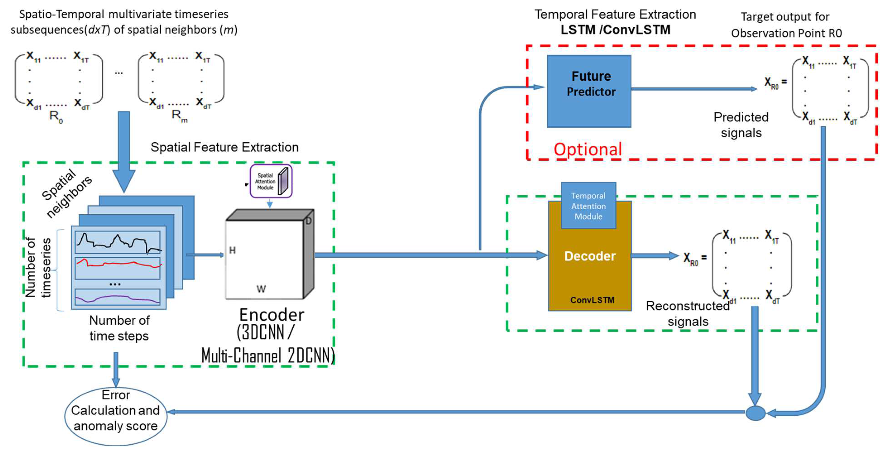
The approach is shown in Figure 1 and is composed of three stages. It starts with the generation of data for the normal case and for cases with pipeline leakages using a hydraulic model for water distribution networks. In this pre-processing stage, a multivariate spatio-temporal dataset is generated so that the deep autoencoder network can exploit the spatial and temporal contexts jointly. The subsequent stage is the data reconstruction and prediction stage, which is executed by a deep hybrid autoencoder network. The autoencoder’s neural network is trained to learn the normal situation using the dataset for the normal case. The third stage is the anomaly detection stage, which is performed based on the reconstruction error. After training, the autoencoder’s neural network can be used to find anomalies (pipeline leaks) in the test dataset. Hereby, a threshold is given on the deviations of the signals from the normal case and violation of the threshold is an indication of an anomaly. These subcomponents will be described in the following sections, starting with data generation.

3.1. Generating Data for Model Training

To accommodate fluctuations in water demand, data noise, and leaks it is necessary to use a hydraulic model for a water distribution system that can consider pressure-driven demand and leakage flow at the pipe level. Various hydraulic models have been developed for this purpose, as mentioned in references [25,26]. The main objective of the standard EPANET implementation, which follows a strict demand-driven approach, is to accurately simulate functioning networks. In this model, water demands are assumed to be predefined inputs. Each node in the model is described by water and energy mass balance equations. The water balance equation (Equation (1)) states that, in the absence of leaks, the inflow of water into a pipe node must be equal to the outflow of water.

$${\sum }_{p\in P_n}{q}_{p,n}-D_n^{act}=0,\forall n\in N$$

(1)

where $P_n$ denotes the set of pipes connected to the node $n$, $q_{p,n}$ is the flow rate of water into node $n$ through pipe p (m³/s), $D_n^{act}$ is the actual water demand at node $n$(m³/s), and $N$ is the number of nodes in the water distribution network.

The total water head, which includes kinetic energy, hydraulic potential energy, and gravitational potential energy, is balanced by the energy. This equation is referenced as [27]. However, when simulating systems with fluctuating water demand, data noise, and pipeline leaks, it is common to have reduced pressures. In these cases, a hydraulic model with Pressure Driven Demand (PDD) consideration is necessary [25]. In a PDD hydraulic model, the values of nodes depend on the local pressure, as shown in Equation (2). The model assumes that each node can be in one of three states: fully served, partially served (with reduced demand), or non-served (with no water withdrawal) when the pressure is zero.

$$D=\left\{\begin{array}{cc}0& p\le P_0\\ D_f{\left(\frac{p-P_0}{P_f-P_0}\right)}^{1/2}& P_0\le p\le P_f\\ D_f& p>P_f\end{array}\right.$$

(2)

where D represents the current demand, $D_f$ represents the desired demand in cubic meters per second (m³/s), p represents the water pressure, $p_f$ represents the pressure at which the desired demand should be met, and $p_0$ represents the minimum water pressure below which no water will be supplied at that location.

The Water Network Tool for Resilience ver. 1.0.0 (WNTR) is a python package that is based on EPANET. It implements the hydraulic network in off-design conditions and is used to construct the water supply network and solve the hydraulic equations [26]. For data collection purposes, the package was utilized to run iteratively with various combinations of random parameters that describe the water supply network in both design and off-design forms. This was achieved by altering the water demand within each range, introducing noise to the data, and simulating leaks in the water distribution network. The leaks are modeled using the orifice Equation (3) [26].

$$d_{leak}=C_{d}A{p}^{\partial }\sqrt{\frac{2}{\rho }}$$

(3)

where $d_{leak}$ is the equivalent water demand due to leak (m³/s), $C_d$ is the discharge coefficient, with a default value 0.75, A is the area of leak, p is the internal water pressure, the exponential $\partial$ is the discharge coefficient, which is 0.5 for steel pipe, and $\rho$ is the water density.

This custom demand described in Equation (3) rapidly increases to a randomized total demand. Such leak demands were placed at random locations and times. The leaks can be either randomly generated or fixed at predefined times and locations. The number and magnitude of leaks can also vary, creating more complex situations. The area values will be chosen randomly between 0.00012 m² and 0.00050 m²; they are the values used in [28]. The ranges for the randomness of water usage, pipe conditions, and data noise were taken from the literature. According to [29], baseline water demand can fluctuate 0.3 times to 1.3 times, depending on the time of the day. The pipe conditions are described with the dimensionless roughness coefficient with values which are uniformly distributed between 100 to 300. Gaussian noise N(0, σ) is added to the water distribution network to account for the uncertainty in the data in general. For the case study, the baseline demand of each service node is taken from the range of 0.008 to 0.012 L/s, assuming a Gaussian distribution with variance σ = 0.01 L/s. Eleven demand ratios from 0.3 to 1.3 are considered during the data generation with the hydraulic model for the WSN. The lower and the upper bounds of the pressure head at the nodes are set to 5 m and 30 m, respectively. Several simulations were conducted for each combination of parameters while recording the water pressure at all nodes. For the test dataset similar simulations were run, but this time some pipelines were cutoff, and data was recorded.

The WNTR simulator needs some improvement in order to avoid memory leaks. The problem is that the simulator saves all intermediate and output data to the RAM, which can easily cause memory overflow. To avoid this, the input data is sliced into segments, saving only the final outputs to the memory. Finally, these outputs are rescaled back to the original timescale.

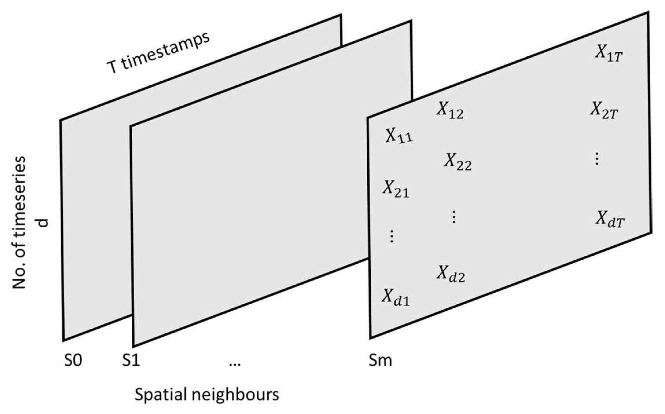
For modelling the individual water networks’ nodes, the nearest neighbor search is applied to each target node to find its nearest neighbors within a given distance, which enables using a limited set of sensors. The distance between nodes is calculated by a Dijkstra path-finding algorithm which finds the closest sensors weighted by their connection length. Using the WNTR simulator, the pressures of the closest nodes are taken as inputs and the target nodes as output. With this data, two modelling approaches can be followed: (1) A model can be created for each target node, or (2) the data of all nodes can be concatenated into a 3D tensor to model all the nodes with one model. The 3D tensor in Figure 2 is built using multivariate time series data from $m$ different spatial sensors $S_i$, where i = 1 … m are the nearest neighbors. The sliding window technique of window size $T$ is used to build the 3-dimensional data. $d$ represents the number of univariate timeseries. The best m can be found empirically for each problem domain.

3.2. Deep Learning Autoencoder

The proposed autoencoder network comprises a 3D convolutional neural network (CNN) and a spatio-temporal decoder component which has a Convolutional Long Short-term Memory (ConvLSTM) network and spatial and temporal attention mechanism. Its structure is shown in Figure 3. The encoder part is based on a 3D CNN, which can capture spatial and temporal features from the input data. It takes in a sequence of 3D volumetric data, which represents the water system condition over time, and extracts relevant features using the convolutional layers. These layers perform convolutions in both the spatial and temporal dimensions, allowing the network to learn spatial and temporal patterns in the data. To effectively use the information related to location and time in the input, we have made modifications to the 3DCNN model by incorporating an attention mechanism. This involves assigning dynamic weights to the input features based on their spatial importance. By utilizing the spatial attention module and temporal attention module, we can dynamically adjust the attention weights, thereby improving the performance of the model.

The decoder part of the network is a Convolutional Long Short-term Memory (ConvLSTM) network. ConvLSTM is an extension of the traditional LSTM architecture that can handle spatio-temporal data. It was introduced in [30] for abnormal event detection and motion estimation in videos, because of its capability to utilize both spatial and temporal information. It uses convolutional operations instead of fully connected layers to process both spatial and temporal information. The ConvLSTM network takes the encoded features from the 3D CNN and decodes them in order to reconstruct the input data.

By combining the 3D CNN and ConvLSTM network, the autoencoder can effectively capture both spatial and temporal dependencies in the input data. This hybrid approach allows for accurate detection of pipe leaks by learning and reconstructing the normal condition of the pipe. Any deviations from the normal condition can be identified as potential leaks.

References [31,32] have shown that combining anomaly detection architectures based on the combination of reconstruction and future prediction make the anomaly detection system robust against noise. Reconstruction methods in autoencoders aim to minimize the reconstruction error for training data, which means they try to reconstruct the input data as accurately as possible. However, this approach may not guarantee large reconstruction errors for abnormal events. Abnormal events may still be reconstructed with relatively low error if they share some similarities with the normal training data. On the other hand, future prediction methods take a different approach. They operate under the assumption that normal events are predictable, meaning that the future instances can be accurately predicted based on past data. In contrast, abnormal events are considered unpredictable, and their future instances cannot be accurately predicted based on the past data. Therefore, in this paper, an approach that combines the methods is developed in order to conduct forecasting and reconstruction sequentially. Forecasting makes the reconstruction errors large enough to facilitate the identification of abnormal events, while reconstruction helps enhance the predicted future from normal events. Specifically, two ConvLSTM network blocks are connected to the decoder part. One block works in the form of forecaster, and the other reconstructs the signals. By focusing on the predictability of future data, this approach can effectively identify abnormal events that are not captured by reconstruction methods.

Overall, the proposed autoencoder network for pipe leak detection combines the strengths of 3D CNN and ConvLSTM to effectively capture and process spatial and temporal information, enabling accurate detection of pipe leaks. Based on 3D convolutional operations on the multivariate spatio-temporal data, the temporal features along with the spatial features can be better preserved. The input data are reconstructed as a 3-dimensional cuboid by stacking multivariate data frames. By applying such an idea, dimensionality reduction, both in a spatial and temporal context, can be achieved for a given input window during the encoding phase.

For each target node, a sample dataset with the water pressure information of its neighborhood generated as previously described is used for training. A total of 70% of the normal non-leaking dataset is normalized and used for training. The remaining 30% of the normal non-leaking dataset is used for validation. For testing the model, the dataset from the leaking conditions is used but normalized based on the mean and variance values of the non-leaking dataset. Hereby, two scenarios were simulated: (1) leak in the target node and (2) leaks in the input pipelines (i.e., leaks in the neighbors).

The 3DCNN-ConvLSTM model is a complex model that requires considerable computational resources to run effectively during inference compared to a Random Forest model or MC-CNN-LSTM. In order to make the model more efficient and suitable for real-time operating conditions, we utilized Dynamic range quantization. Dynamic range quantization is a technique used to reduce the computational complexity of a model by quantizing the weights and activations to a lower precision format. This reduces the memory footprint and computational requirements of the model without significantly sacrificing its performance. By applying dynamic range quantization to the 3DCNN-ConvLSTM model, we were able to achieve a noticeable improvement in computation speed. Specifically, the model’s inference time on a CPU was reduced by 1.28 times compared to running the model without quantization. This means that the model can now process data faster, making it more suitable for real-time applications.

3.3. Anomaly Detection Stage (Leak Detection)

In this stage, the anomalies (leaks) are found by calculating the sum of the reconstruction and forecasting errors as anomaly score. For a model trained by a dataset of only non-leak conditions, a large reconstruction error occurs if data of leaking conditions are supplied at the input, because the relationship described by the trained AE neural network is not valid under such conditions. By setting a threshold in the construction error, the AE model can classify if a set of data corresponds to a leaking situation or a non-leaking situation.

Let $x=\left\{x\right(1),x(2),...,x(T\left)\right\}$ and $y=\left\{y\right(1),y(2),...,y(H\left)\right\}$ be univariate time series data representing one of the reconstructed features and its forecasts, and T and H are the length of the input and prediction windows, respectively. Each data point $x\left(i\right)$ represents a data reading for that feature at time instance $t_i$. The mean absolute error (MAE) is used to calculate the reconstruction and forecast error for the given period (input window + prediction window) for each feature as

$$MAE(x)=1/T{\sum }_T\left|x_i-{\widehat{x}}_i\right|+1/H{\sum }_H\left|x_i-{\widehat{x}}_i\right|$$

(4)

where $x_i$ is the observed value and ${\widehat{x}}_i$ is the reconstructed value at time instance $t_i$.

Dynamic threshold adjustment based on the moving averages is used to continuously update the threshold based on the latest observations.

To deal with exceptions, we used three different methods in the real case. After the initial anomaly detection, a post-processing step is performed to refine the results. We applied statistical tests, considering temporal dependencies, and incorporating domain knowledge to validate and filter out false positives. We also involved human experts to evaluate the end results. They provided domain-specific knowledge to identify and interpret anomalies that may be falsely captured by automated methods. Lastly, we could employ a combination of different anomaly detection algorithms (our model and the two baselines) to increase the chances of detecting anomalies effectively. As will be seen, each algorithm has its strengths and weaknesses, so using multiple approaches can provide a more comprehensive analysis.

3.4. Baselines

Two baselines were considered for comparison with our method. The first baseline MC-CNN-LSTM is also based on unsupervised learning. It consists of two main components: the MC-CNN-Encoder and the LSTM decoder. The MC-CNN-Encoder is responsible for extracting spatial features from the input data, while the LSTM decoder captures temporal dependencies and reconstructs the sequence data. The MC-CNN-Encoder is composed of two convolutional blocks, each containing four layers. The first layer is a 2D convolutional layer with a kernel size of (2 × 2) and 16 filters. This layer applies a set of filters to the input data, extracting spatial features. Zero-padding is used to maintain the spatial dimensions of the input. The output of the convolutional layer is then passed through an activation layer, which introduces non-linearity to the feature maps. This helps in capturing complex patterns and relationships in the data. Next, a 2D max-pooling layer is applied to the feature maps. This layer reduces the spatial dimensions of the input by half, using a pool size of (2 × 2) and strides of (2 × 2). Max-pooling selects the maximum value within each pooling region, further highlighting important features. Finally, a channel-wise batch normalization layer is applied to normalize the feature maps across different channels. This helps in improving the stability and generalization of the model. The second convolutional block follows a structure similar to the first block, but with a larger kernel size of (3 × 3) and 32 filters. This allows for capturing more complex spatial features. The output of the MC-CNN-Encoder is a set of spatial feature maps that are dependent on previous time steps. To capture these temporal dependencies, the LSTM decoder is utilized.

The LSTM decoder takes the feature maps from the MC-CNN-Encoder and processes them through an LSTM block. The LSTM block consists of memory cells that can store and update information over time. This allows the model to capture long-term dependencies in the input sequence. The output of the LSTM block is then passed through a fully connected neural network (FCNN) layer. This layer maps the LSTM output to the desired output sequence, reconstructing the original sequence data.

The second baseline model is based on the random forest (RF) algorithm designed by Leo Breiman, which combines the results of several decision trees. The random forest is an extremely random tree regressor, which is different from the way that standard decision trees (DTs) are built. When looking for the best split to separate the samples of a node into two groups, random splits are drawn for each of the randomly selected features, and the best split among those is chosen. According to the data structure described in the data processing section, the RF model was realized according to how the spatial information was incorporated. Coordinate grids as engineered features were generated and added as extra columns. The RF was implemented and optimized in Python using Bayesian Optimization. A grid of hyperparameter ranges was defined, a random sample was taken from the grid, and a K-Fold CV was performed with each combination of values. The random forest model’s parameters (max_depth, max_features, min_samples_leaf, min_samples_split, and n_estimators) were tuned during cross validation. The following parameters were found: max_depth = 70, min_samples_leaf = 4, min_samples_split = 10, and n_estimators = 100 for the case studies.

3.5. Evaluation

The anomaly score in the proposed method is calculated based on two factors: (1) the difference in gradient between the model (for early detection) and the real values and (2) the mean absolute error. The difference in gradient measures the deviation between the predicted values from the model and the actual values in the water distribution network. A larger difference indicates a higher likelihood of an anomaly or abnormal behavior in the system. The mean absolute error, on the other hand, quantifies the average magnitude of the errors between the predicted and actual values. A higher mean absolute error suggests a higher level of uncertainty or inaccuracy in the model’s predictions. By combining these two factors, the anomaly score provides a comprehensive assessment of the deviation and uncertainty in the system. A higher anomaly score indicates a higher probability of an anomaly or abnormal event occurring in the water distribution network. For anomaly detection, the value of the threshold of the reconstruction and forecast errors for deciding whether values are anomalies need to be determined. Therefore, a statistics histogram of reconstruction and forecast errors in non-leaking and leaking conditions was constructed for the case study to see whether the two conditions are separable. For localization of the pipe leaks, the individual errors of the individual features are examined to find the feature with the maximum contribution to Equation (4). Further spatial attention weights generated by the attention mechanism are analyzed to find the relationships between the nodes. These weights indicate the importance or relevance of different regions or pipes in the network for leak localization. The attention weights are visualized to gain insights into the network’s behavior. This is completed by overlaying the attention weights on a map of the water distribution network and highlighting the pipes with high attention weights. These areas are likely to have leaks or require further investigation.

As the target nodes take their neighbors’ information as inputs, the presence of large errors in the target node can result from themselves having leaks or their neighbors. Once a target node is identified as anomalous or abnormal, additional investigation is conducted by examining its neighboring nodes. The purpose of this investigation is to determine the exact cause or source of the anomaly. By analyzing the information received from the neighbors, researchers aim to identify whether the target node itself is responsible for the error or if it is caused by the information received from its neighbors.

This approach allows for the detection of leaks and other anomalies in the system by identifying instances where the anomaly score exceeds a certain threshold. By monitoring the anomaly score over time, it is possible to detect and respond to anomalies promptly, minimizing the impact on the network and improving its overall performance.

4. Results

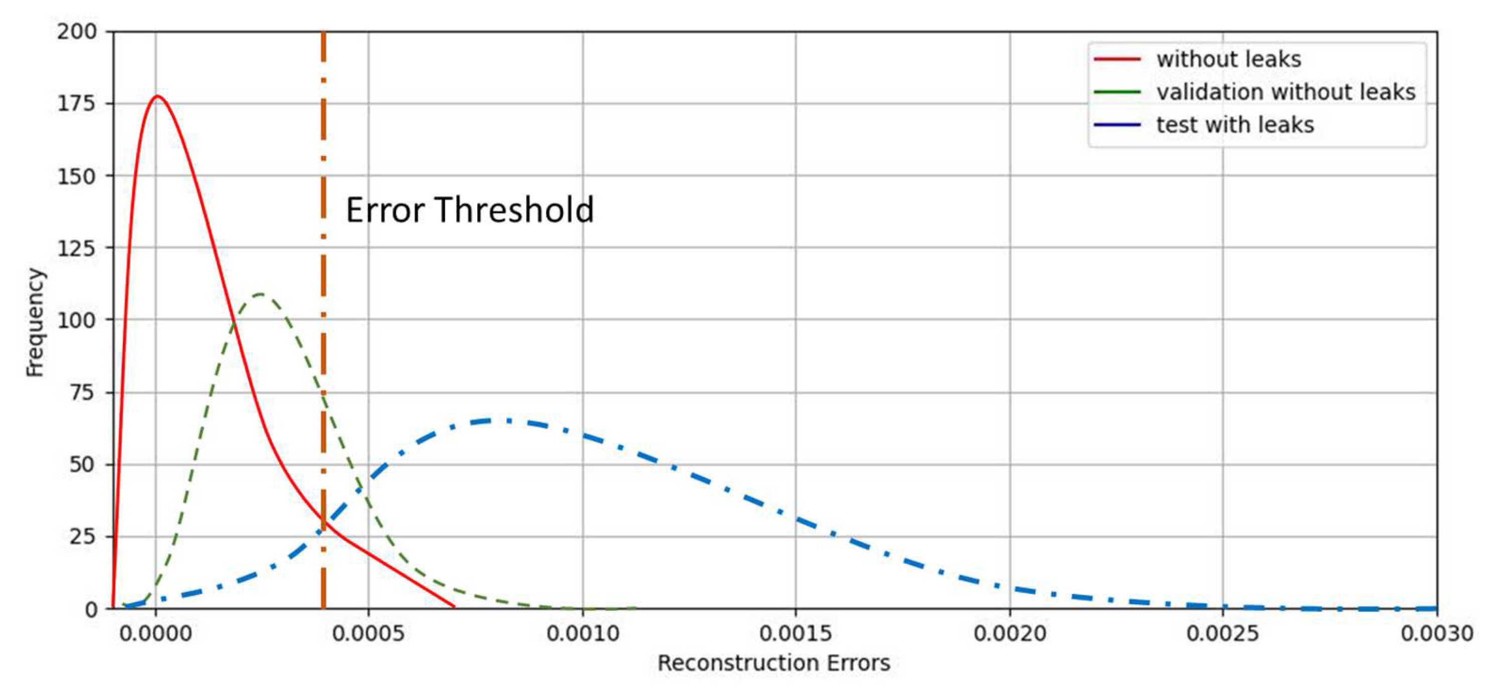
The hydraulic model of the D-Town WSN is built using the WNTR software Version 1.0.0. The model considers the actual water demands at each node and simulates both non-leaking and leaking scenarios in order to generate the necessary data sets for evaluating the leak detection algorithm. The results are as follows: The histogram of the reconstruction errors of the non-leaking and leaking conditions is shown in Figure 4. The reconstruction error of data under normal non-leaking situation is small, with 97.5% of reconstruction error, which is less than 1.5 × 10⁻³. The validation of the dataset under leaking conditions shows large reconstruction errors. Fortunately, this clear difference in behavior makes the selection of the threshold values much easier. The difference can be used to define the threshold for leak detection. Figure 4 shows that, for the case study, a threshold of reconstruction error of 4 × 10⁻³ can be used to differentiate the leak versus non-leak situations.

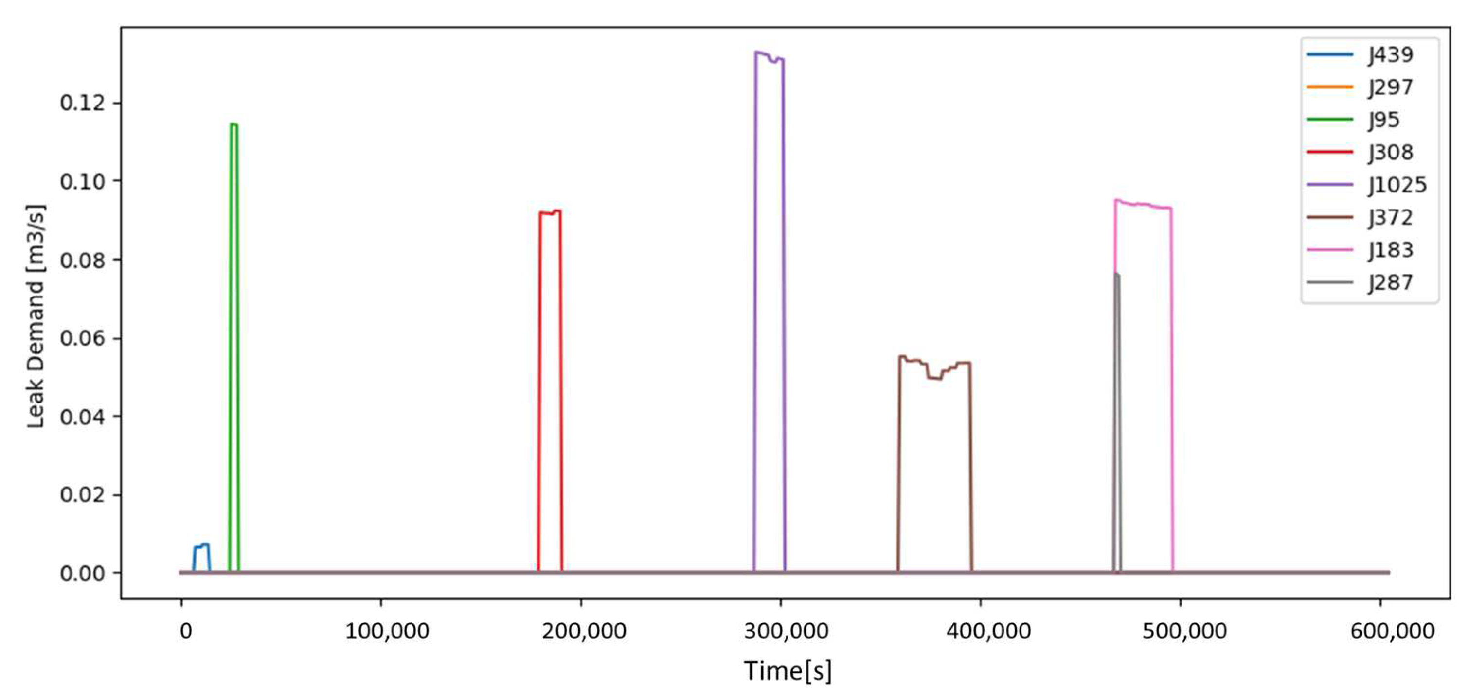
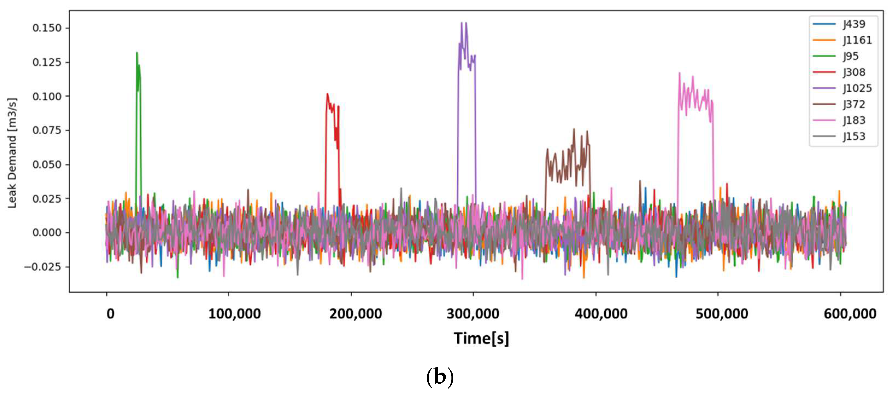
To evaluate the network under leak conditions, the network has been subjected to various leak scenarios over a period of one week, each with different characteristics. Some leaks showed a gradual increase in flow over time, while others had a sudden and immediate appearance. Figure 5 provides a visual representation of the flow behavior for each node where leaks were simulated.

The data indicates that the leaks were not clustered together but rather occurred at spaced intervals. However, there was also a situation where leaks happened simultaneously in different locations, specifically at nodes J372 and J1025. Overall, this information highlights the complexity and diversity of the leak scenarios that were simulated on the network.

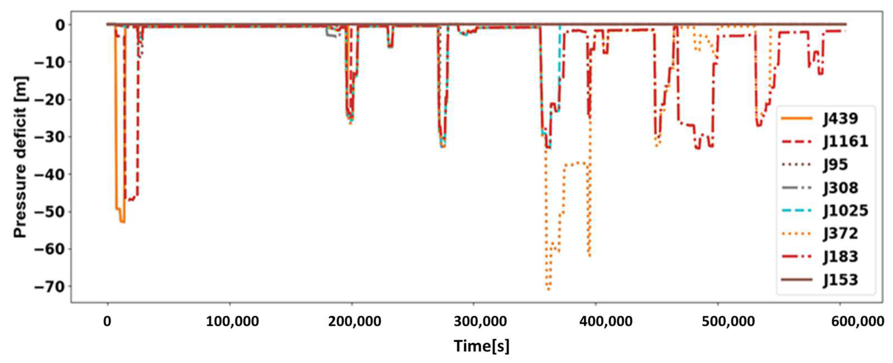
Figure 6 provides valuable information about the behavior of the water distribution system during both normal operation and leak events and shows the values of the pressure deficit throughout the simulation over time. The pressure deficit is an important parameter to monitor as it indicates the difference between the actual pressure in the network and the desired pressure. In a well-functioning system, the pressure deficit should be minimal and within acceptable limits. However, during leak events, the pressure deficit increases significantly, indicating a drop in pressure. By examining Figure 5, it is possible to identify the moments when there are leaks in the system. These are indicated by high pressure deficits, which correspond to a sudden drop in pressure. This information is crucial for leak detection, as it allows for the timely identification of leaks and the implementation of appropriate measures for repair and maintenance and allows for the evaluation of the effectiveness of the leak detection method.

Overall, the analysis of Figure 6 demonstrates the importance of monitoring pressure deficits and other system parameters to detect and evaluate the impact of leaks. The visualization provided by these plots allows for a better understanding of the behavior of the system during normal operation and leak events, enabling effective leak detection and management.

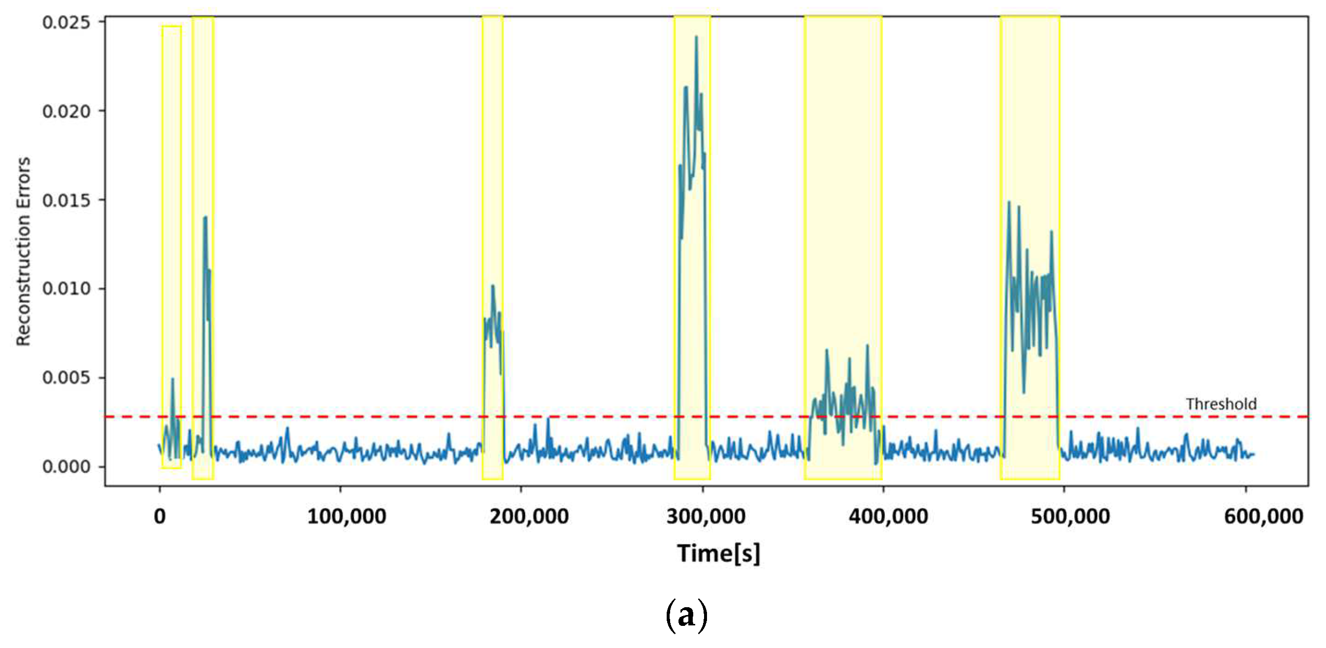
The discussion continues with the analysis of Figure 7a, which demonstrates that the proposed method successfully detects all the leaks in the network and accurately predicts their duration. This is a crucial aspect of leak detection as it allows for timely repairs and maintenance to be carried out. Figure 7b provides further insight into the causes of the detected leaks, showing that they correspond to the registered causes. This indicates that the method can accurately identify the sources of the leaks, which is essential for effective leak management and mitigation.

To provide a comprehensive evaluation of the method’s performance, an unbalanced dataset of size 6375 is used as input, out of which only 13% (834) specifically pertains to leakage signals. Hereby, a data ratio of 60/20/20 is used in the training, validation, and test of the model. The resulting confusion matrix of our method is presented in

Table 1. Confusion matrix.

	Non Leakage Prediction			Leakage Prediction
	Our Method	RF	MC-CNN-LSTM	Our Method	RF	MC-CNN-LSTM
Non leakage reality	1063 (0.96)	930 (0.84)	1019 (0.92)	45 (0.04)	191 (0.15)	101 (0.08)
Leakage reality	0.0	19 (0.01)	14 (0.01)	166 (1.0)	134 (0.81)	140 (0.10)

. This matrix summarizes the results and allows for a better understanding of the classification accuracy. It shows the number of true positives, true negatives, false positives, and false negatives, providing a quantitative assessment of the method’s performance. With this unbalanced data, our method shows a true–false rate of only 4%, compared to the random forest (RF) model showing 15% false positives and 0.01% false negatives and the MC-CNN-LSTM showing 8% false positives. The random forest method shows, as expected, that it ignores fewer classes even though the data for the random forest method was improved using the Synthetic Minority Over-Sampling Technique for Regression with Gaussian Noise (SMOGN).

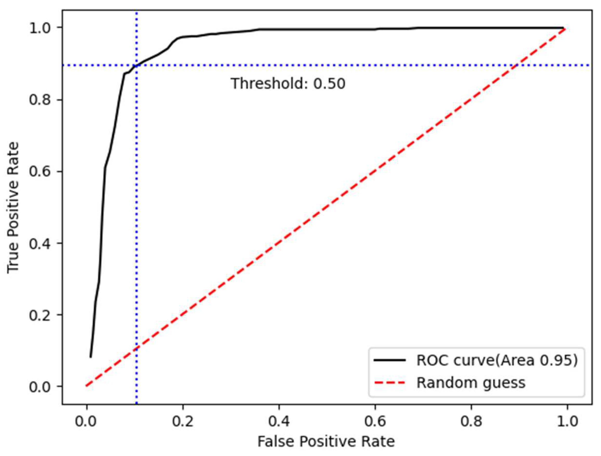
Additionally, the Receiver Operating Characteristic (ROC) curve in Figure 8 illustrates the trade-off between the true positive rate (sensitivity) and the false positive rate (1-specificity) at different classification thresholds. The ROC curve is a common tool used to evaluate the performance of classification models. A higher area under the curve (AUC) indicates a better performance of the method in distinguishing between positive and negative instances.

Overall, the analysis of Figure 7a,b, Figure 8, and Table 1 demonstrates that the proposed method is effective in detecting and classifying leaks in the water distribution network. It accurately identifies the leaks, predicts their duration, and provides insights into their causes. This information can be used to prioritize repairs, allocate resources efficiently, and ultimately reduce water loss in the network.

The evaluation of the confusion matrix in terms of accuracy reveals that the detection method achieved an 86% score. According to reference [33], this indicates a high level of accuracy in leak detection. This suggests that the proposed leak detection process in this research ensures a reliable detection rate using existing monitoring data. The methodology proposed is straightforward and efficient, demonstrating its effectiveness in leak detection. The analysis of the leaks, which were classified false positive and false negative showed that the majority of the leaks were of short duration, less than thirty minutes, or the leakage area was very small, less than 0.0001 m². Furthermore, the poor classification also happened in time instants where that water demand fluctuations were high.

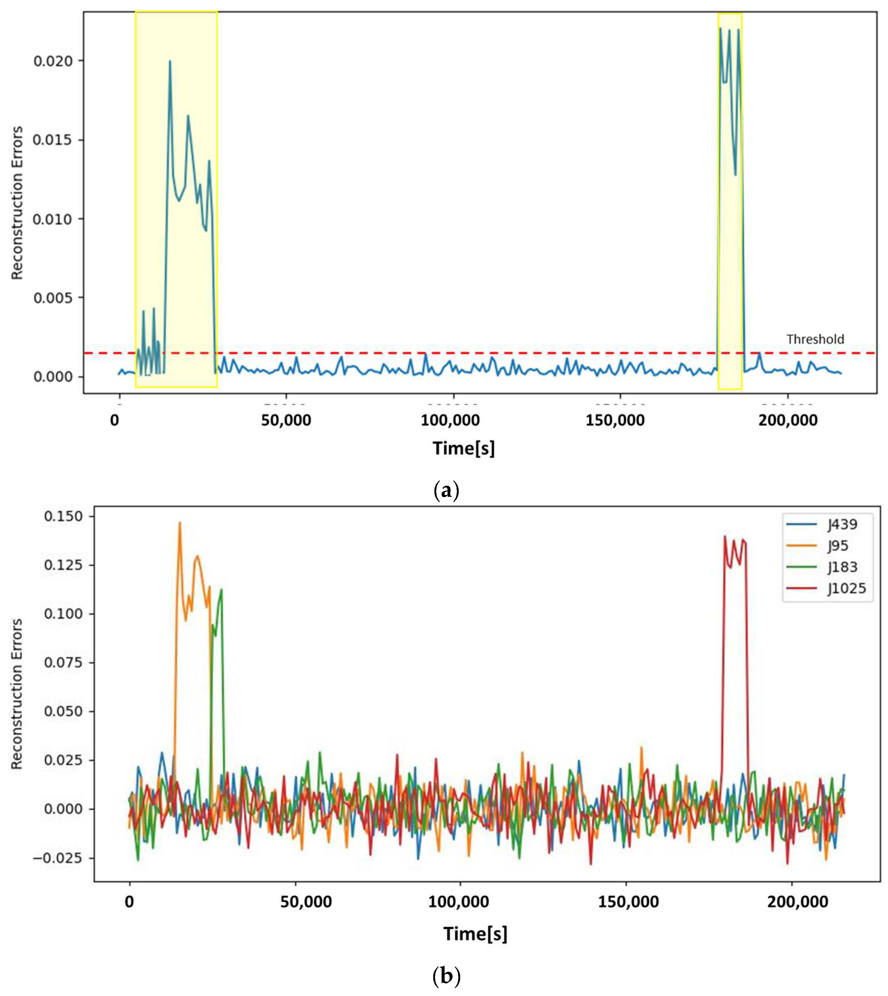
The second case study presented in the discussion highlights the effectiveness of the model in detecting and predicting leaks in a real network. In the second case study, the training dataset consisted of 5680 samples, while the validation and test sets had sizes of 1274 and 2116 samples, respectively. However, since there were only seven recorded instances of leakages in the real case, all of them were included in the test dataset. This means that the test dataset contained only the seven samples with leakages, while the remaining samples were distributed between the training and validation sets. In this case, four leaks were registered in pipes ‘J439’, ‘J95’, ‘J183’, and ‘J1025’ over a period of 60 h. These leaks occurred at different times and some of them overlapped.

Figure 9a illustrates the reconstruction and forecast errors of the model when applied to this test case. It is observed that the model performs well in detecting and predicting the leaks, as the errors are relatively small for most of the period. However, there are two noticeable periods where large errors are observed, namely from 2 to 8 h and from 50 to 52 h.

To further investigate the causes of these errors, Figure 9b provides an analysis. It is evident that the main causes of the errors are the pipes where the leaks occurred, namely ‘J439’, ‘J95’, ‘J183’, and ‘J1025’. This finding is expected, as these pipes were the ones where the leaks were registered.

Overall, this case study demonstrates the practical applicability of the model in real-world scenarios. The model successfully detects and predicts leaks in the network, with only a few instances of larger errors. This suggests that the model can be easily deployed and utilized to effectively manage and maintain water distribution networks, ultimately reducing water loss and improving overall system efficiency.

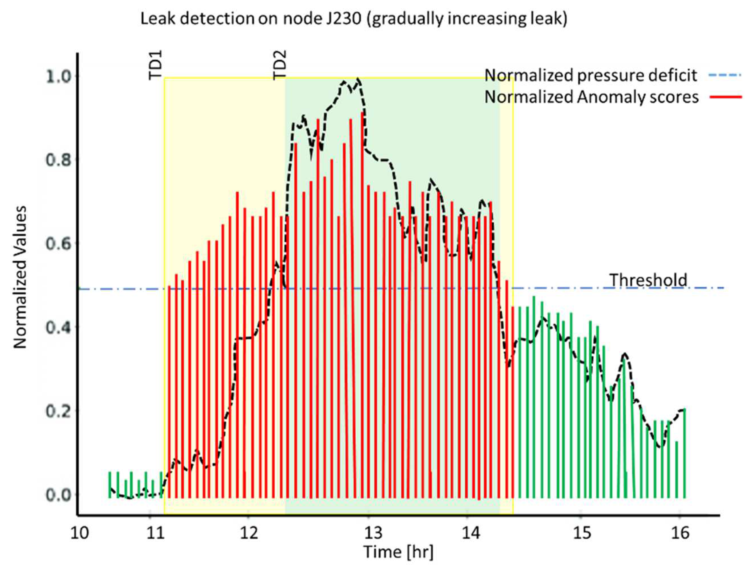
The detection time of the leak is a critical factor in leak management, as it directly impacts the efficiency and effectiveness of the response. By detecting the leak early, the necessary repairs can be carried out promptly, minimizing the impact on the water distribution system and reducing the potential for further damage or water loss. Therefore, the second case study was also used to analyze the detection time of the leaks. This is especially important for leaks which develop with time. A leak on node J230 resembles this feature and the results of detection are shown in Figure 10. This leak is of particular interest as it develops over time, making it crucial to detect it as early as possible to minimize water loss and potential damage.

The graph shows the detection time of the leak on node J230 over a period of 60 h. It is observed that the proposed method successfully detects the leak at around 11.3 h, almost an hour earlier (TD1) than the simple pressure threshold method (TD2), and accurately predicts its duration. This early detection allows for prompt action to be taken to repair the leak and prevent further water loss.

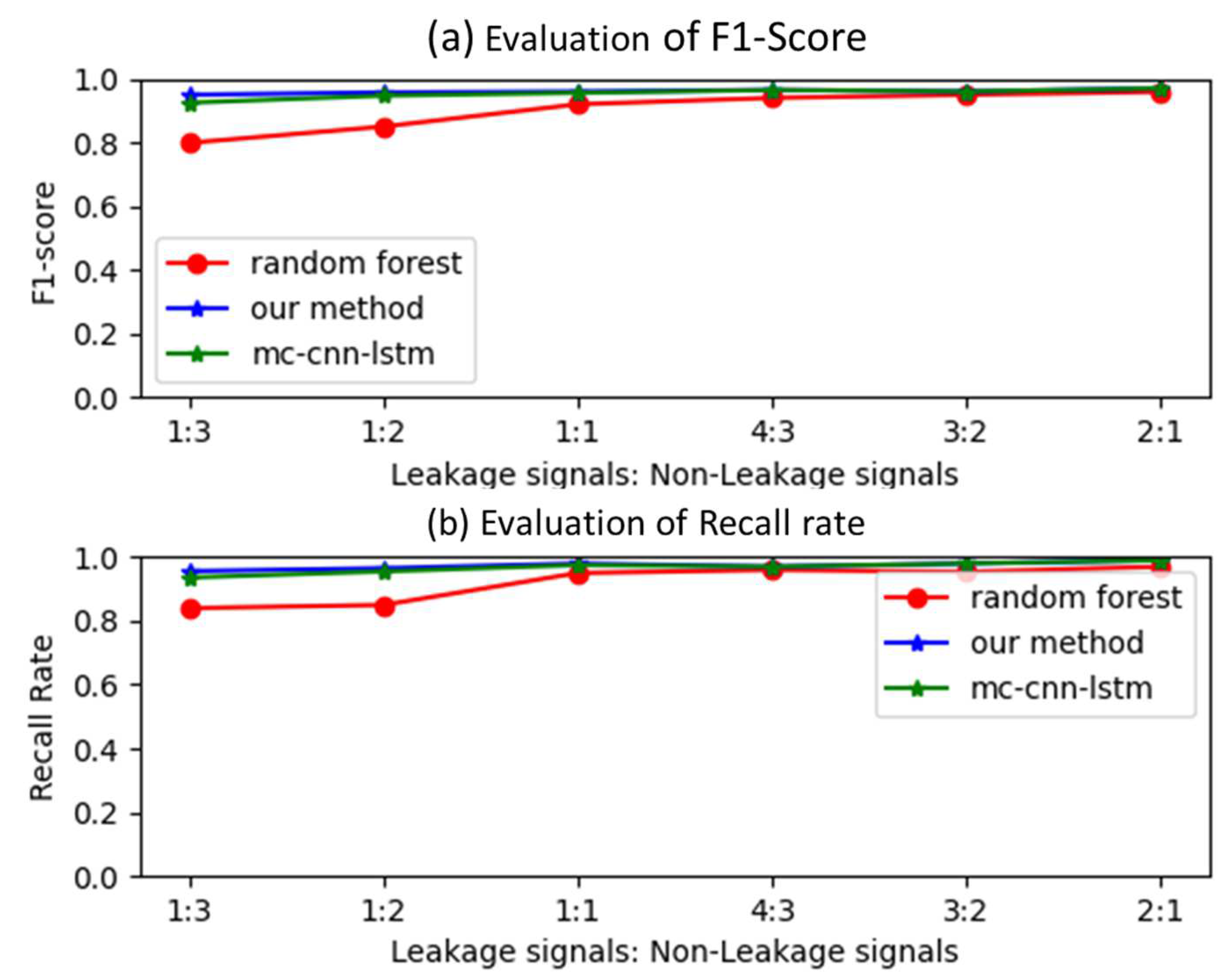
Furthermore, the principle of balanced class is fundamental in most machine learning models, as it ensures that all classes are given equal importance. However, unbalanced input data present a challenge as they can cause the models to overlook the minority classes. In the context of leak detection, the number of leakage signals is significantly lower than the number of non-leakage signals. To address this, the study analyzed the ratio of leakage to non-leakage signals in the training dataset and compared it to a random forest model based on supervised learning after applying Synthetic Minority Over-Sampling Technique for Regression with Gaussian Noise (SMOGN) to find the optimal over- and undersampling necessary to improve the data. The models were then trained and evaluated using different ratios, including 1:3, 1:2, 1:1, 4:3, 3:2, and 2:1. The evaluation results are depicted in Figure 9 for recall rate and F1-score. Figure 11a,b demonstrates that the evaluation metrics of the machine learning models exhibit patterns similar to the proportion of data variations. Our method is hardly affected by the ratio of the leakage to non-leakage conditions. As for the supervised learning-based random forest model, as the proportion approaches 1 to 4:3, the changes in the evaluation metrics become less pronounced. When the proportion of leakage to non-leakage signals is less than one, the recall rate and F1 value decrease rapidly, indicating a decline in the models’ classification performance. On the other hand, when the proportion exceeds 4:3, there is no significant improvement in the evaluation metrics as the ratio increases. However, it is important to note that collecting more leakage data would increase the cost of data acquisition. Therefore, this study chooses to train the random forest model with a proportion of one for the input data.

5. Discussion

The literature reviews have indicated that detecting leaks in water distribution networks is a complex task that requires significant computational resources and real-time capabilities. The main challenges arise from a lack of monitoring data, noisy data, and intermittent water demand. Fluctuations in water demand make it difficult for computer algorithms to differentiate between non-leaking and leaking conditions. Traditional methods such as using inspection tools or physical models are expensive, labor-intensive, and cannot achieve real-time detection. Additionally, implementing physical models in wireless sensor networks (WSN) is challenging due to the complex topology and uncertainty in hydraulic conditions, requiring domain expertise.

An alternative approach, commonly found in the literature, is leak detection using transient responses. However, this method requires capturing transient signals during the short period when a leak occurs, necessitating a high sampling rate. A more promising approach in the era of artificial intelligence is the use of data-driven methods that utilize machine learning models. These approaches can provide real-time and reliable leak detection. The rationale behind these methods is that the spatial pattern of water pressure and its variations under leak conditions are influenced by the network structure of the water distribution system and should be considered in leak detection.

In this study, a hybrid autoencoder model is proposed, which incorporates both spatial and temporal information for leak detection. This model can detect leaks even with unbalanced data, meaning it can work with data collected under normal operational conditions. Additionally, the model utilizes multiple sensor nodes for detection, making it more robust than data-driven models that only use data from a single node. The proposed method can provide near real-time leak detection with high accuracy and does not require extensive domain expertise to implement. Unlike leak detection based on transient signals, which necessitates high sampling rates, the autoencoder model learns from the spatial patterns in the data and only requires sensors with low sampling rates. While data used for model training and validation in this study are from data generated by a high fidelity model for WSN. The framework is readily applied to real-world data as could be shown in the second case study.

Here are some key findings and results from our study using 3DCNN ConvLSTM autoencoders for spatial-temporal pipe leak detection:

• Improved detection accuracy: The combination of 3DCNNs and ConvLSTMs has been found to improve the accuracy of leak detection compared to traditional methods. The network can effectively capture spatial features and temporal dynamics, enabling the detection of subtle changes in flow and pressure patterns caused by leaks.
• Early detection of leaks: The 3DCNN ConvLSTM autoencoder has shown the ability to detect leaks at an early stage, even before they become significant and easily detectable through traditional methods. This early detection can help prevent further damage and reduce water loss.
• Accurate leak localization: The network’s ability to capture spatial information allows for accurate leak localization. By comparing the input and output frames, the network can identify the specific pipes or areas where leaks are likely to be located. This enables targeted repair and maintenance actions, reducing the time and effort required for leak detection and repair.
• Robustness to noise and variations: The 3DCNN ConvLSTM autoencoder has demonstrated robustness to noise and variations in the data. It can handle fluctuations in flow rates, pressure levels, and other factors that may affect the accuracy of leak detection. This robustness improves the reliability of the system in real-world operating conditions.
• Generalizability across networks: The 3DCNN ConvLSTM autoencoder has been shown to be applicable to different types of water distribution networks, including networks with varying sizes, pipe materials, and topologies. This generalizability makes it a versatile approach that can be implemented in various contexts.

While the results of using 3DCNN ConvLSTM autoencoders for spatial-temporal pipe leak detection are promising, there are still some challenges and limitations. These include the need for large and diverse training datasets, the computational complexity of the network architecture, and the requirement for accurate and reliable sensor data.

Overall, the use of 3DCNN ConvLSTM autoencoders for spatial-temporal pipe leak detection in water distribution networks offers a data-driven approach that can improve the accuracy, early detection, and localization of leaks. Further research and development in this area can lead to more effective and efficient leak detection systems for sustainable water management.

6. Conclusions

In conclusion, this paper highlights the importance of leak detection in water distribution networks and emphasizes the need for water companies to minimize water loss and improve efficiency. The proposed method utilizes a hybrid framework of an autoencoder, combining a 3D convolutional neural network (CNN) and a spatio-temporal decoder component called a Convolutional Long Short-term Memory (ConvLSTM) network.

By considering the spatial and temporal relationship of water pressure at multiple nodes in a water distribution network, the autoencoder network successfully detects leaks. The inclusion of spatial and temporal attention modules further enhances the accuracy of both leak detection and localization.

To validate the effectiveness of the proposed method, data for the experiments is generated using the WNTR simulator, which incorporates pressure-driven demand nodes, leaking conditions, fluctuating water demand, and data noise based on the EPANET hydraulic model. The results of the leak detection experiments on benchmark and real case studies, along with the comparison with two baselines, demonstrate the robustness and high accuracy of the developed model in detecting leaks.

Overall, this paper provides valuable insights into the application of deep learning techniques for leak detection in water distribution networks. The proposed method shows great potential for practical implementation by water companies to minimize water loss and improve operational efficiency.