Fault Diagnosis of Oil-Immersed Transformers Based on the Improved Neighborhood Rough Set and Deep Belief Network

Abstract

As one of the essential components in power systems, transformers play a pivotal role in the transmission and distribution of renewable energy generation. Accurate diagnosis of transformer fault types is crucial for maintaining the safety of power systems. The current focus in research lies in transformer fault diagnosis methods based on Dissolved Gas Analysis (DGA). Traditional diagnostic methods directly utilize the five fault gases from DGA data as model input features, but this approach does not comprehensively reflect all potential fault types in transformers. In this paper, a non-coding ratio method was employed to generate 35 fault gas ratios based on the five fault gases, subsequently refined through correlation analysis to eliminate redundant feature variables, resulting in 15 significantly representative fault gas ratios. To further streamline the feature variables and remove non-contributing elements to fault diagnosis, an improved Neighborhood Rough Set (INRS) algorithm was introduced, leveraging symmetrical uncertainty measurement. By resorting to the proposed INRS, eight most representative fault gas ratios were selected as input variables for constructing a Deep Belief Network (DBN) diagnostic model. Experimental results on Dissolved Gas Analysis (DGA) data confirmed the effectiveness and accuracy of the proposed method.

1. Introduction

Oil-immersed transformers are essential components of power systems and play a critical role in the transmission and distribution of electrical energy [1,2]. However, prolonged operation and high-load conditions can lead to a deterioration in equipment performance, and even severe damage, posing a threat to the stability and reliability of power systems [3,4]. Traditional transformer maintenance and inspection primarily rely on periodic inspections and tests, but this approach may not detect internal potential faults in a timely manner, leading to overlooked or delayed maintenance and increased risk and maintenance costs. To take effective maintenance and preventive measures in a timely manner, accurate prediction of fault types becomes increasingly important [5,6].

Dissolved Gas Analysis (DGA) is one of the most commonly used methods for diagnosing faults in oil-immersed transformers [7]. During the operation of transformers, chemical reactions occur in the oil–paper composite insulation materials, releasing low-molecular-weight gases such as hydrogen, hydrocarbons, and carbon-containing gas compounds, which dissolve in the insulating oil [8,9]. Different types of faults or abnormal conditions result in the production of different gases, with the most significant ones being hydrogen (${\mathrm{H}}_2$), methane (${\mathrm{CH}}_4$), ethane (${\mathrm{C}}_2{\mathrm{H}}_6$), ethylene (${\mathrm{C}}_2{\mathrm{H}}_4$), and acetylene (${\mathrm{C}}_2{\mathrm{H}}_2$). Based on the type and quantity of fault gases, it is possible to determine the presence of specific fault types in the transformer [10]. Traditional diagnostic methods, such as the IEC three-ratio method, Doernenberg ratio method, and Rogers ratio method, encode faults based on the ratios of fault gases and associate them with fault types to diagnose transformer fault types [11,12,13]. However, in practice, it is possible to encounter fault combinations that fall outside the coding range, making traditional diagnostic methods unable to accurately diagnose transformer fault types.

Learning from data is a core research area in modern artificial intelligence [14]. Machine learning-based fault diagnosis techniques have been successfully applied to predict fault types in oil-immersed transformers. Typical intelligent diagnostic approaches encompass the BP neural network [15], Support Vector Machine (SVM) model [16], and other methods. An approach that integrates neural networks with the three-ratio method was introduced in [17], which is designed to transform samples with diagnostic errors from neural networks to the three-ratio method for diagnosis. Nevertheless, the accuracy of neural network judgments relies on the choice of weights and thresholds, demanding substantial training data, which complicates the operation and compromises stability. The study in [18] presented an intelligent diagnosis approach for transformer faults, which combines empirical wavelet transform and an enhanced convolutional neural network. The findings indicate that this diagnostic model can proficiently recognize the fault states of transformers. In [19], a novel multiclass probabilistic diagnosis framework for dissolved gas analysis, based on Bayesian networks and hypothesis testing, was proposed. This framework learns patterns from data and infers the uncertainty associated with diagnostic outcomes. In [20], SVM was employed to establish a classification system for power transformer faults and to select the most suitable gas signature between traditional DGA methods and a novel extension method. This approach led to significant improvements in the accuracy of power transformer fault classification. It is worth noting that both [19] and [20] used the traditional set of five fault gases (${\mathrm{H}}_2$, ${\mathrm{CH}}_4$, ${\mathrm{C}}_2{\mathrm{H}}_6$, ${\mathrm{C}}_2{\mathrm{H}}_4$, and ${\mathrm{C}}_2{\mathrm{H}}_2$) as input variables for the diagnostic models. However, these five feature variables contain incomplete fault information, resulting in lower diagnostic accuracy. In order to fully leverage the fault information embedded in the fault gases, Dai et al. employed a non-coding ratio method to derive nine fault feature gas ratios. These nine features were then used as input variables for a deep belief network, resulting in a notable enhancement in diagnostic accuracy [21]. Currently, fault diagnosis techniques based on machine learning and deep learning are still evolving. Continual learning methods are discussed in reference [22]. Integrated approaches are highlighted in reference [23] and have demonstrated promising results in fault diagnosis.

This paper constructed 35 fault feature gas ratios based on five fault gases and eliminated redundant features through correlation analysis. To further reduce the number of features contributing insignificantly to transformer faults and consequently simplify the model, an improved neighborhood rough set (INRS) algorithm was proposed. Compared to the traditional approach of directly using the five fault gases as feature variables, the feature reduction method introduced in this study can effectively harness the fault information inherent in these five fault gases. The eight features extracted through the INRS algorithm contribute more significantly and representatively to the types of transformer faults. Using the obtained ratios of eight characteristic gases as input variables, a deep belief network (DBN) diagnostic model was constructed. The average accuracy of 10 experiments on the DGA test set reached 90.2%.

2. Transformer Fault Characteristics Analysis

Currently, traditional power distribution systems extensively utilize oil-immersed electrical transformers, which are commonly classified into three main fault types: mechanical, thermal, and electrical. As mechanical faults might appear as thermal or electrical faults, our focus is solely on non-mechanical fault categories. The specific fault categories pertaining to oil-immersed transformers are described in

Table 1. Types of faults in oil-immersed transformers.

Faults	Specific Fault Types
Thermal Faults	MLTO (Medium-low-Temperature Overheating)
	HTO (High-Temperature Overheating)
Electrical Faults	PD (Partial Discharge)
	LED (Low-Energy Discharge)
	HED (High-Energy Discharge)
Mechanical Faults	Manifests as Thermal Faults or Electrical Faults

.

Thermal faults or electrical faults in transformers are primarily reflected in the changes in the concentration of various gases dissolved in the oil. The most significant of these gases include hydrogen (${\mathrm{H}}_2$), methane (${\mathrm{CH}}_4$), ethane (${\mathrm{C}}_2{\mathrm{H}}_6$), ethylene (${\mathrm{C}}_2{\mathrm{H}}_4$), and acetylene (${\mathrm{C}}_2{\mathrm{H}}_2$). The distinctive gas concentration features for different fault types are outlined in

Table 2. Gas content of different fault types in oil-immersed transformers.

Fault Type	Gas Content
MLTO	Total hydrocarbon content ${\mathrm{CH}}_4$ is high, with ${\mathrm{C}}_2{\mathrm{H}}_4$ and ${\mathrm{C}}_2{\mathrm{H}}_2$ making up about 2%.
HTO	High total hydrocarbon content, with ${\mathrm{C}}_2{\mathrm{H}}_4$ accounting for less than 5.5% of the total, and ${\mathrm{H}}_2$ representing roughly 27% of the total hydrocarbon content.
PD	Elevated levels of ${\mathrm{H}}_2$, ${\mathrm{CH}}_4$, and ${\mathrm{C}}_2{\mathrm{H}}_6$.
LED	Elevated levels of ${\mathrm{C}}_2{\mathrm{H}}_4$, ${\mathrm{C}}_2{\mathrm{H}}_2$, and ${\mathrm{H}}_2$. The total hydrocarbon content is not high, with ${\mathrm{C}}_2{\mathrm{H}}_2$ representing more than 25% of the total hydrocarbon content, while ${\mathrm{H}}_2$ exceeds 90% of the total hydrogen content.
HED	High ${\mathrm{C}}_2{\mathrm{H}}_2$ and elevated ${\mathrm{H}}_2$ levels. Extremely high total hydrocarbon content, with ${\mathrm{C}}_2{\mathrm{H}}_2$ comprising 18% to 65%, being the predominant component of the total hydrocarbon content.

.

From Table 2, it is apparent that different fault types often lead to the release of specific gases. Analyzing the gases dissolved in the oil both qualitatively and quantitatively enables insights into the operational status and potential fault types present within the transformer. Consequently, Dissolved Gas Analysis (DGA) serves as a valuable method for diagnosing fault types in transformers within power distribution systems. Typically, datasets containing concentrations of the five fault gases along with their associated fault types are referred to as DGA data. These data facilitate the identification and assessment of transformer conditions, aiding in predictive maintenance and timely fault detection.

3. Fault Diagnosis of Oil-Immersed Transformers Based on INRS and DBN

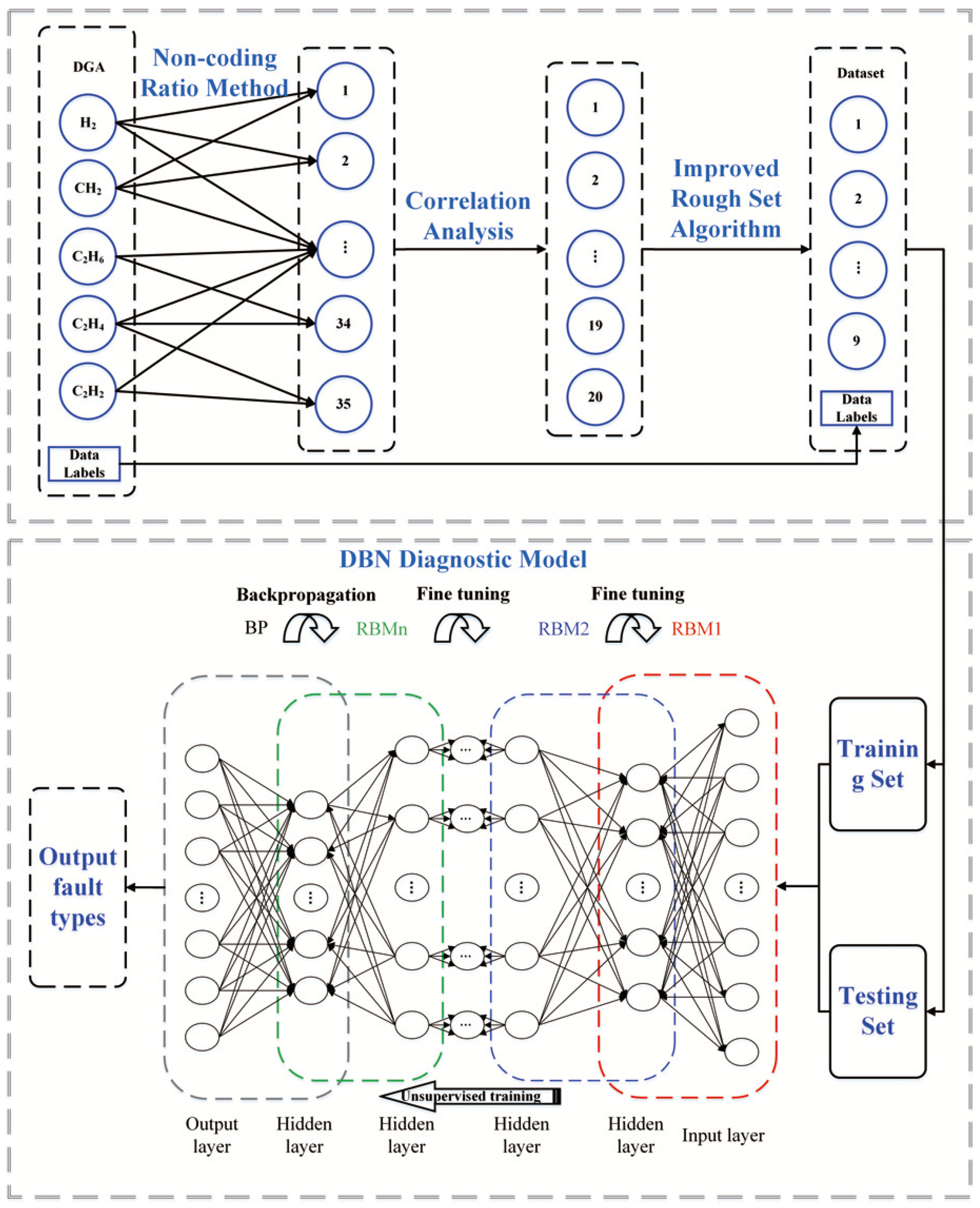
Based on the analysis in the previous section, the fault types of oil-immersed transformers can be summarized as six categories: LED, HED, PD, HTO, MLTO, and Normal. Consequently, the fault diagnosis problem for oil-immersed transformers can be treated as a six-class classification task. To accomplish this classification task, we have constructed a DBN diagnostic model based on the proposed INRS algorithm. The overall framework is illustrated in Figure 1. DGA data contain historical data on the content of five fault gases in oil-immersed transformers under different fault types, which can be used for model training in transformer fault diagnosis. The DGA data used in this paper can be obtained from https://github.com/Cliango/DGA.git (accessed on 20 July 2023). The dataset contains a total of 617 samples, including 102 LEDs, 168 HEDs, 47 PDs, 133 HTOs, 77 MLTOs, and 90 Normal samples. The specific distribution of data samples can be found in

Table 3. Distribution of DGA data samples.

Fault Types	LED	HED	PD	HTO	MLTO	Normal	Total
Number of Samples	102	168	47	133	77	90	617

. Each sample consists of gas content of five fault gases: ${\mathrm{H}}_2$, ${\mathrm{CH}}_4$, ${\mathrm{C}}_2{\mathrm{H}}_6$, ${\mathrm{C}}_2{\mathrm{H}}_4$, and ${\mathrm{C}}_2{\mathrm{H}}_2$.

3.1. Non-Coding Ratio Processing

Conventional methods for diagnosing transformer faults using fault gases from DGA data (such as the IEC three-ratio method, Doernenberg ratio method, and Rogers ratio method) have demonstrated the utility of gas ratios in fault diagnosis for oil-immersed transformers. Additionally, there is a close connection between the changes in the proportion of fault gases and the fault types. Hence, gas ratios among the five fault gases can be utilized as features to analyze and determine the internal operational status of the transformer. The five basic fault gases alone cannot fully reflect the fault information of the transformer. To further explore the fault information, a total of 35 gas ratios have been constructed using a non-coding ratio method, as outlined in

Table 4. Ratios of feature gas concentrations.

Number	Ratios	Number	Ratios	Number	Ratios	Number	Ratios
1	${\mathrm{C}}_2{\mathrm{H}}_2/{\mathrm{H}}_2$	10	${\mathrm{C}}_2{\mathrm{H}}_2/{\mathrm{C}}_2{\mathrm{H}}_4$	19	${\mathrm{C}}_2{\mathrm{H}}_2/\mathrm{C}$	28	${\mathrm{C}}_2{\mathrm{H}}_4/{\mathrm{HC}}_1$
2	${\mathrm{C}}_2{\mathrm{H}}_6/{\mathrm{H}}_2$	11	${\mathrm{H}}_2/{\mathrm{C}}_2$	20	${\mathrm{C}}_2{\mathrm{H}}_4/\mathrm{C}$	29	${\mathrm{C}}_2{\mathrm{H}}_6/{\mathrm{HC}}_1$
3	${\mathrm{C}}_2{\mathrm{H}}_4/{\mathrm{H}}_2$	12	${\mathrm{CH}}_4/{\mathrm{C}}_2$	21	${\mathrm{C}}_2{\mathrm{H}}_2/\mathrm{HCC}$	30	${\mathrm{C}}_2{\mathrm{H}}_2/{\mathrm{HC}}_1$
4	${\mathrm{C}}_2{\mathrm{H}}_2/{\mathrm{H}}_2$	13	${\mathrm{C}}_2{\mathrm{H}}_6/{\mathrm{C}}_2$	22	${\mathrm{C}}_2{\mathrm{H}}_4/\mathrm{HCC}$	31	${\mathrm{C}}_2{\mathrm{H}}_2/{\mathrm{HC}}_2$
5	${\mathrm{C}}_2{\mathrm{H}}_6/{\mathrm{CH}}_4$	14	${\mathrm{C}}_2{\mathrm{H}}_4/{\mathrm{C}}_2$	23	${\mathrm{C}}_2{\mathrm{H}}_6/\mathrm{HCC}$	32	${\mathrm{C}}_2{\mathrm{H}}_4/{\mathrm{HC}}_2$
6	${\mathrm{C}}_2{\mathrm{H}}_4/{\mathrm{CH}}_4$	15	${\mathrm{C}}_2{\mathrm{H}}_2/{\mathrm{C}}_2$	24	${\mathrm{CH}}_4/\mathrm{HCC}$	33	${\mathrm{C}}_2{\mathrm{H}}_6/{\mathrm{HC}}_2$
7	${\mathrm{C}}_2{\mathrm{H}}_2/{\mathrm{CH}}_4$	16	${\mathrm{H}}_2/\mathrm{C}$	25	${\mathrm{H}}_2/\mathrm{HCC}$	34	${\mathrm{CH}}_4/{\mathrm{HC}}_2$
8	${\mathrm{C}}_2{\mathrm{H}}_4/{\mathrm{C}}_2{\mathrm{H}}_6$	17	${\mathrm{CH}}_4/\mathrm{C}$	26	${\mathrm{CH}}_4/{\mathrm{HC}}_1$	35	${\mathrm{H}}_2/{\mathrm{HC}}_2$
9	${\mathrm{C}}_2{\mathrm{H}}_2/{\mathrm{C}}_2{\mathrm{H}}_6$	18	${\mathrm{C}}_2{\mathrm{H}}_6/\mathrm{C}$	27	${\mathrm{H}}_2/{\mathrm{HC}}_1$

$\mathrm{C}={\mathrm{C}}_1+{\mathrm{C}}_2$, ${\mathrm{HC}}_1={\mathrm{H}}_2+{\mathrm{C}}_1$, ${\mathrm{HC}}_2={\mathrm{H}}_2+{\mathrm{C}}_2$, $\mathrm{HCC}={\mathrm{H}}_2+{\mathrm{C}}_1+{\mathrm{C}}_2$.

. Here, ${\mathrm{C}}_1$ represents first-order hydrocarbons (i.e., ${\mathrm{CH}}_4$), and ${\mathrm{C}}_2$ represents the sum of second-order hydrocarbons (i.e., ${\mathrm{C}}_2{\mathrm{H}}_6+{\mathrm{C}}_2{\mathrm{H}}_4+{\mathrm{C}}_2{\mathrm{H}}_2$).

Although we conducted non-coding ratio processing on five types of fault gases, resulting in 35 ratios indicative of these faults and allowing for a more comprehensive reflection of transformer fault types, it is important to note that these features may exhibit linear relationships among themselves. To avoid introducing redundant feature variables, we performed a correlation analysis among the 35 features, further eliminating highly correlated feature variables to streamline the input features of the model.

Let $D={\{x_i,y_i\}}_{i=1}^{617}$ represent the dataset obtained after non-coding ratio processing of the DGA data, where $x_i=[x_{i1},x_{i2},\cdots ,x_{i35}]$ is the i-th sample, $x_{ij}$ represents the j-th feature within the sample $x_i$, and $y_i\in \{Normal,MLTO,HTO,PD,LED,HED\}$. Using all 35 feature gas ratios as input features may result in high dimensionality, increasing the complexity of the diagnostic model. Moreover, an excessive number of input features can introduce interference from features with low correlation, potentially affecting the diagnostic accuracy. Therefore, before establishing the diagnostic model, feature selection and dimensionality reduction are essential to ensure the model’s efficiency and accuracy while avoiding unnecessary interference. To achieve this, a Pearson correlation analysis is first applied to the data D, eliminating features that exhibit linear relationships, thereby preventing the introduction of redundant information or multicollinearity. Let data matrix $X=[x_1^T,x_2^T,\cdots ,x_{617}^T]$, where the i-th row of X (i.e., $X_i$) represents the i-th feature of the samples. The correlation coefficient between any two features can be calculated by

$$R(X_i,X_j)=\frac{{\sum }_{k=1}^n(X_{ik}-{\mu }_{X_i})(X_{jk}-{\mu }_{X_j})}{n{S}_{X_i}{S}_{X_j}},$$

(1)

where ${\mu }_{X_i}$ and $S_{X_i}$ represent the mean and variance of $X_i$, respectively. The correlation coefficient R has a range between −1 and 1. When R is close to 1 (−1), it indicates a stronger positive (negative) correlation between features $X_i$ and $X_j$. When R is close to 0, it signifies no linear correlation between the two features. In this paper, we remove the gas ratio features in the data where $\left|R\right|\ge 0.7$. The reason for removing feature gas ratios with correlation coefficients greater than 0.7 is that during the feature selection process, we noticed that coefficients exceeding 0.7 may indicate strong linear relationships among features, thereby introducing multicollinearity, which can affect the model’s robustness and interpretability. However, through a series of experiments, we found that setting the correlation coefficient threshold to 0.7 effectively streamlined the model, maintaining a high diagnostic accuracy while efficiently reducing model complexity by avoiding excessive redundant information. This strategy not only enhanced the model’s interpretive capacity but also improved the overall experimental outcomes and diagnostic precision.

The results indicate that there are 20 gas ratio features with correlation coefficient $\left|R\right|\ge 0.7$, specifically, features numbered 2, 3, 6, 9, 16, 19, 21–23, and 25–35 in Table 4. These features exhibit strong linear correlations with each other. To avoid introducing redundant information, these features are removed from the dataset D, resulting in the dataset $\overline{D}$, containing 15 gas ratio features. After removing linearly correlated feature gas ratios, there are a total of 15 remaining, as detailed in

Table 5. Gas ratio features after reduction through correlation analysis.

Number	Ratios	Number	Ratios
1	${\mathrm{C}}_2{\mathrm{H}}_2/{\mathrm{H}}_2$	10	${\mathrm{C}}_2{\mathrm{H}}_2/{\mathrm{C}}_2{\mathrm{H}}_4$
4	${\mathrm{C}}_2{\mathrm{H}}_2/{\mathrm{H}}_2$	14	${\mathrm{C}}_2{\mathrm{H}}_4/{\mathrm{C}}_2$
5	${\mathrm{C}}_2{\mathrm{H}}_6/{\mathrm{CH}}_4$	15	${\mathrm{C}}_2{\mathrm{H}}_2/{\mathrm{C}}_2$
7	${\mathrm{C}}_2{\mathrm{H}}_2/{\mathrm{CH}}_4$	17	${\mathrm{CH}}_4/\mathrm{C}$
8	${\mathrm{C}}_2{\mathrm{H}}_4/{\mathrm{C}}_2{\mathrm{H}}_6$	18	${\mathrm{C}}_2{\mathrm{H}}_6/\mathrm{C}$
10	${\mathrm{C}}_2{\mathrm{H}}_2/{\mathrm{C}}_2{\mathrm{H}}_4$	20	${\mathrm{C}}_2{\mathrm{H}}_4/\mathrm{C}$
11	${\mathrm{H}}_2/{\mathrm{C}}_2$	24	${\mathrm{CH}}_4/\mathrm{HCC}$
12	${\mathrm{CH}}_4/{\mathrm{C}}_2$	25	${\mathrm{H}}_2/\mathrm{HCC}$
13	${\mathrm{C}}_2{\mathrm{H}}_6/{\mathrm{C}}_2$

$\mathrm{C}={\mathrm{C}}_1+{\mathrm{C}}_2$, ${\mathrm{HC}}_1={\mathrm{H}}_2+{\mathrm{C}}_1$, ${\mathrm{HC}}_2={\mathrm{H}}_2+{\mathrm{C}}_2$, $\mathrm{HCC}={\mathrm{H}}_2+{\mathrm{C}}_1+{\mathrm{C}}_2$.

.

3.2. Feature Selection Based on the Improved NRS

Correlation analysis can eliminate redundant information between features, but to comprehensively assess the importance of features, it is essential to examine the relationship between features and the target variable, i.e., the correlation between features and the target variable. In general, features that exhibit a higher correlation with the target variable are more likely to contribute to the predictive capability of the model. The neighborhood rough sets (NRS) algorithm is a data mining algorithm based on rough set theory, used for feature selection and data reduction. It evaluates each attribute by calculating attribute importance, thereby eliminating redundant information and unimportant attributes from the dataset while retaining the most valuable attributes.

For a decision system $DS=(U,C\cup E,V,f)$, where U is the universe of discourse, C represents conditional attributes, $E\ne ⌀$ is the set of decision attributes, and $C\cup E\ne ⌀$, $V=\left\{V_a\right|a\in C\cup E\}$ denotes the collection of attributes’ values. The information function $f:U\times (C\cup E)\to V$ represents the mapping relationship between samples, attributes, and attribute values. In this paper, the set composed of feature gases represents the set of conditional attributes, denoted as C, while the set consisting of the five fault types serves as the set of decision attributes. Let B be a subset of conditional attributes, specifically, a subset of all feature gases. For any $B\subseteq C$, the dependency of decision attributes E on conditional attributes B is defined as

$${\gamma }_B\left(E\right)=\frac{|Po{s}_B\left(E\right)|}{\left|U\right|},$$

(2)

where $Po{s}_B\left(E\right)$ represents the lower approximation of the attribute subset. The formula for calculating the importance of a certain conditional attribute to the decision attribute is

$$sig\left(a\right)={\gamma }_B\left(E\right)-{\gamma }_{B-\left\{a\right\}}\left(E\right).$$

(3)

The NRS have certain limitations and drawbacks in feature selection. When the number of samples varies significantly across different classes within the dataset, the NRS might exhibit bias towards classes with larger sample sizes, impacting the feature selection process. Moreover, these methods heavily rely on dataset partitioning, leading to potentially different outcomes based on various data splits, thus affecting the consistency and stability of feature selection. Symmetrical Uncertainty (SU) is a measure based on information theory, designed to quantify the association between features and target variables. As a metric for feature selection, SU aids in assessing the correlation between features and target variables, enabling the identification of influential features impacting the target. By eliminating highly correlated features, it mitigates multicollinearity, reducing the risk of model overfitting and enhancing model generalization. The application of SU facilitates the reduction of feature dimensions while retaining critical features, thus streamlining the model and improving its efficiency. The introduction of SU as an alternative method helps overcome some of the limitations associated with domain rough set methods.

Let $\overline{D}=[{\overline{D}}_1,\cdots ,{\overline{D}}_i,\cdots ,{\overline{D}}_{15}]\in {\mathbb{R}}^{617\times 15}$ be the data matrix after the correlation analysis in Section 3.1, where ${\overline{D}}_i\in {\mathbb{R}}^{617}$ for $i\in \{1,2,\cdots ,15\}$ represents the i-th feature after reduction. The SU value between the 15 gas ratio features and the label vector can be calculated using the following formula:

$$SU({\overline{D}}_i,Y)=2·\frac{IG({\overline{D}}_i,Y)}{H\left({\overline{D}}_i\right)+H\left(Y\right)},$$

(4)

where Y is the vector of the class label for sample, $IG({\overline{D}}_i,Y)=H\left({\overline{D}}_i\right)-H\left({\overline{D}}_i\right|Y)$ represents information gain, and $H\left({\overline{D}}_i\right)$ represents information entropy. By incorporating the measure of uncertainty (4) into the attribute importance (3), we have developed a rough set-based attribute reduction method based on SU

$$SUSIG({\overline{D}}_i,Y)=\frac{1}{2}(sig\left({\overline{D}}_i\right)+SU({\overline{D}}_i,Y)).$$

(5)

By incorporating SU into the attribute importance assessment within the NRS algorithm, we have developed an improved neighborhood rough set algorithm used to evaluate the correlation between feature variables and the target variable (i.e., label vector).

The main steps of this algorithm are as follows:

Step 1: Data normalization.

Step 2: Calculate the attribute importance SUSIG for 15 attributes according to (5), and sort the attributes in descending order based on SUSIG, $red={\varphi }_0$, and the sorted attributes are denoted as $C=\{a_1,\cdots ,a_{15}\}$.

Step 3: Taking the attribute $a_1\in C$ with the highest attribute importance as the initial reduction, denoted as $re{d}_1=re{d}_0\cap \left\{a_1\right\}$, calculate $P_{OS}$ according to (2), and set $red=re{d}_1$.

Step 4: Neighborhood construction. Calculate the standard deviation $Std\left(a_i\right)$ for each attribute $a_i$, and construct the neighborhood radius $\delta =\left(Std\left(a_i\right)\right)/\tau$, where $\tau$ is a predetermined parameter used to adjust the neighborhood size, typically ranging from 2 to 4. Based on the importance of attributes, select a set of the most important attributes to form the neighborhood, creating a neighborhood rough set.

Step 5: Set $i=i+1$ and $re{d}_i=re{d}_{i-1}\cap \left\{a_i\right\}$. Calculate ${\gamma }_B\left(E\right)$ according to (2) and set $B=re{d}_i$. If ${\gamma }_{B_{i-1}}\left(E\right)<\left|{\gamma }_{B_i}\left(E\right)\right|$, then $red=re{d}_i$ and proceed to the next step; otherwise, stop.

Step 6: Data reduction. Utilize the neighborhood rough set for data reduction, eliminating redundant information and unimportant attributes from the dataset while retaining the most valuable attributes.

In order to minimize the reduced features, we set the parameter $\tau =2$. Subsequently, the algorithm steps described above are applied to the dataset $\overline{D}$, leading to the removal of low-importance gas ratio features. The result is a set of 8 gas ratio features that exhibit high correlation with the fault labels, as detailed in

Table 6. Gas ratio features after reduction through INRS.

Number	Ratios	Number	Ratios
7	${\mathrm{C}}_2{\mathrm{H}}_2/{\mathrm{CH}}_4$	17	${\mathrm{CH}}_4/\mathrm{C}$
11	${\mathrm{H}}_2/{\mathrm{C}}_2$	18	${\mathrm{C}}_2{\mathrm{H}}_6/\mathrm{C}$
13	${\mathrm{C}}_2{\mathrm{H}}_6/{\mathrm{C}}_2$	24	${\mathrm{CH}}_4/\mathrm{HCC}$
15	${\mathrm{C}}_2{\mathrm{H}}_2/{\mathrm{C}}_2$	25	${\mathrm{H}}_2/\mathrm{HCC}$

$\mathrm{C}={\mathrm{C}}_1+{\mathrm{C}}_2$, ${\mathrm{HC}}_1={\mathrm{H}}_2+{\mathrm{C}}_1$, ${\mathrm{HC}}_2={\mathrm{H}}_2+{\mathrm{C}}_2$, $\mathrm{HCC}={\mathrm{H}}_2+{\mathrm{C}}_1+{\mathrm{C}}_2$.

.

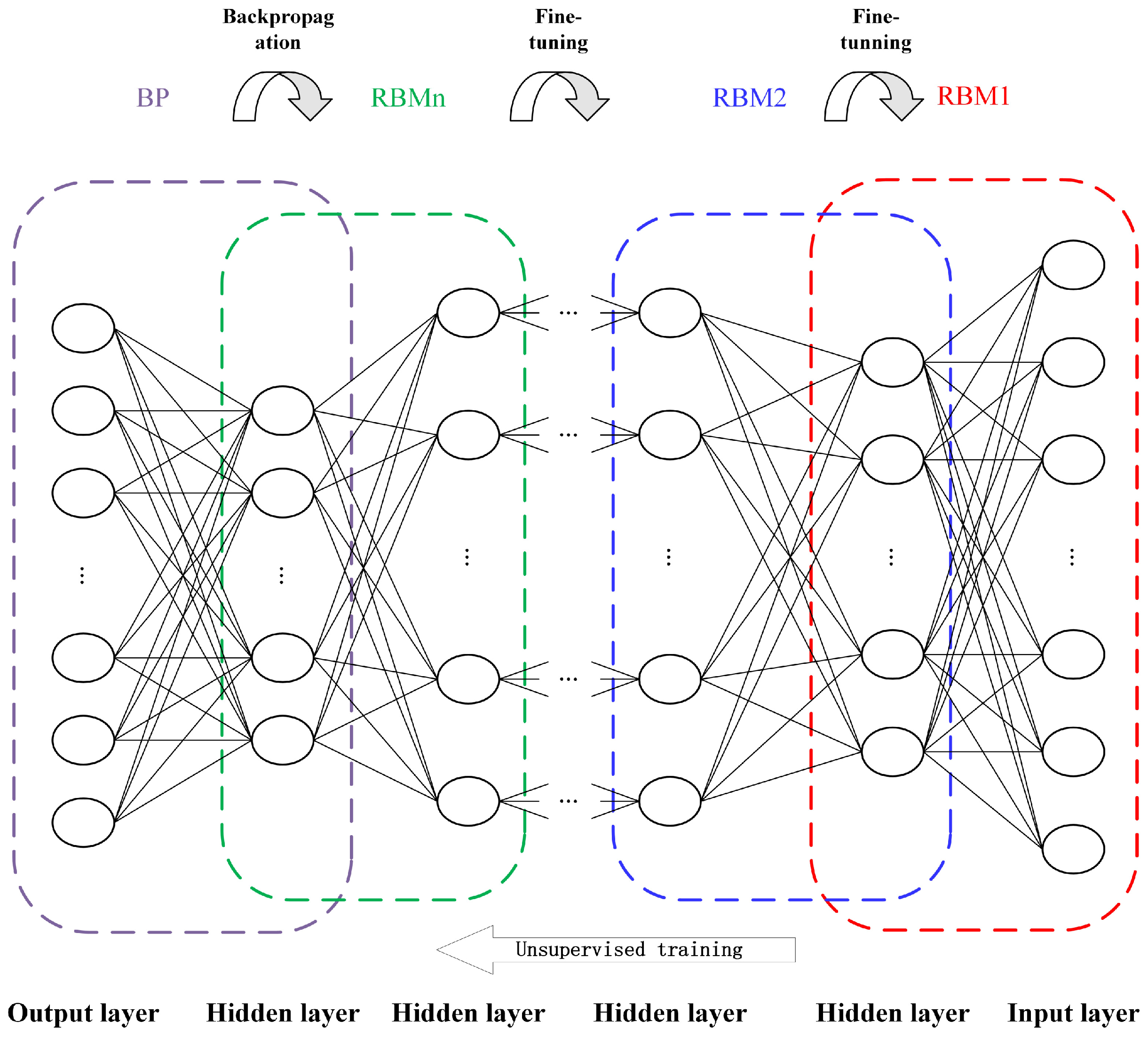
3.3. Transformer Diagnostic Model Based on DBN

DBN is a deep learning model constructed by stacking multiple Restricted Boltzmann Machines (RBM). The network structure is illustrated in Figure 2.

Each RBM consists of two layers of neurons, with the visible layer receiving input data and the hidden layer used to capture abstract features of the data. The training process of a DBN comprises two phases: unsupervised pre-training and fine-tuning.

Unsupervised Pre-Training: Starting from the bottom, each RBM is trained layer by layer. The hidden layer’s output of each RBM is used as the visible layer input for the next RBM. Through parameter updates, it reconstructs the distribution of the input data. During this process, network connection weights between neurons with the smallest reconstruction error are chosen, resulting in a new hidden layer for RBM1. This new hidden layer is then employed as the visible layer for training RBM2. This process continues, stacking multiple layers of RBMs to extract data features. The goal is to make the final feature representation as close as possible to the distribution of the original input data. Throughout the pre-training process, no labels of the data are used, making this phase an unsupervised learning process. The pseudocode in Algorithm 1 describes the training process of the DBN model.

Algorithm 1: Deep Belief Network (DBN)

1: DBN Initialize: 2: Initialize weights and biases for each layer 3: Set learning rate and other hyperparameters 4: Train RBM Layer: 5: for each RBM layer do 6:    Train RBM with input data 7:    Update weights and biases 8: end for 9: Build DBN: 10: for each layer in DBN do 11:    Train RBM layer with input data 12: end for 13: Fine-Tune DBN: 14: Fine-tune the entire DBN using backpropagation or other optimization algorithms 15: Update all weights and biases

Fine-Tuning: While the DBN model can establish initial deep features through layer-wise pre-training, it cannot guarantee the attainment of globally optimal deep feature representations since each RBM is trained independently to minimize the reconstruction error. To further optimize the entire DBN model and ensure the acquisition of superior deep feature representations, it is common to add a back-propagation network connected to a classifier at the end of the DBN. This is conducted for fine-tuning. The fine-tuning process employs supervised learning, using labeled data to adjust the parameters of the entire DBN, including the weights and biases, in order to minimize the classifier’s loss function. This way, the entire DBN model can better adapt to a specific classification task and obtain improved feature representations.

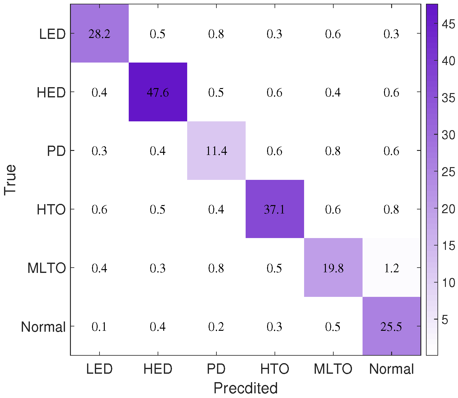
We use a DBN to perform the classification task of oil-immersed transformer fault types. The six fault types, namely, LED, HED, PD, HTO, MLTO, and Normal, are encoded as (1, 0, 0, 0, 0, 0), (0, 1, 0, 0, 0, 0), (0, 0, 1, 0, 0, 0), (0, 0, 0, 1, 0, 0), (0, 0, 0, 0, 1, 0), and (0, 0, 0, 0, 0, 1), respectively. The nine gas ratio features, which have been reduced through correlation analysis and the INRS algorithm as discussed in Section 3.2, are used as the input layer for the DBN, while the five fault type encodings serve as the output layer. The complete steps for oil-immersed transformer fault diagnosis are as follows:

Step 1: Collect the dissolved gas analysis data of various fault gases during the operation of oil-immersed transformers.

Step 2: Conduct non-coding ratio processing for the fault gases in the data to obtain 35 gas ratio features.

Step 3: Remove redundant features through correlation analysis and normalize the data. Utilize the Neighborhood Rough Sets algorithm for feature selection to eliminate features that have minimal contributions to fault types, optimizing the feature set.

Step 4: Split the processed data into training and testing sets in a certain proportion to ensure the independence of model training and evaluation.

Step 5: Use the selected gas ratio features and binary-encoded fault types as the input and output layers of the DBN, respectively. Determine the DBN network parameters, including the number of network layers, learning rate, and the number of neurons in the hidden layers.

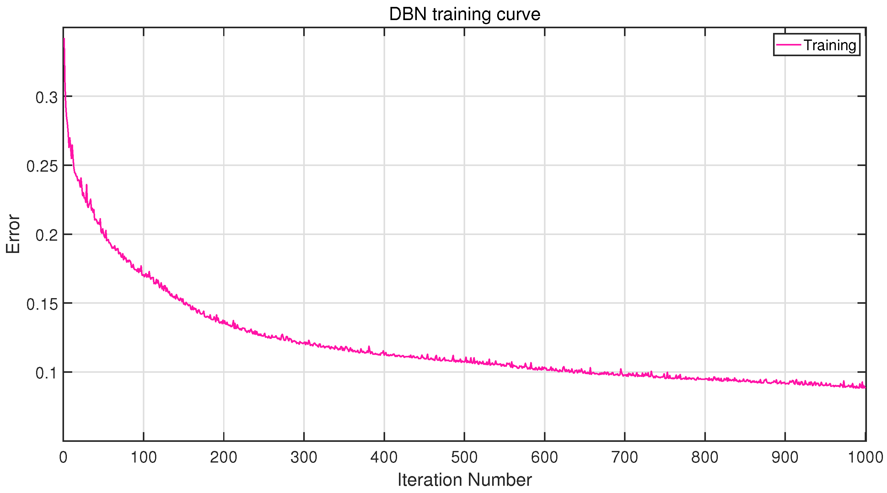
Step 6: Pre-train and fine-tune the DBN network until reaching the specified number of training iterations or the desired error threshold to complete the DBN fault diagnosis model. Input the test data into the model to obtain the output results.

When training a DBN, it is necessary to set and select network parameters such as the number of network layers, learning rate, and the number of neurons in the hidden layers, as mentioned in Step 5. Properly configuring these network parameters can optimize the DBN model and improve its performance and effectiveness. Since there are no fixed rules or criteria to determine the best parameters, experimentation and practical trials are required to continuously try and optimize to find the most suitable parameter configuration.

According to Figure 2, in the processed data, each class of samples is divided into a testing set and a training set in a 7:3 ratio, with 70% of the data used for training and 30% for testing the model’s performance. In the model, the learning rate for RBMs is set to 0.01. This learning rate is used during the pre-training process and controls the rate at which the RBM network weights are updated to gradually converge to better feature representations. In the BP fine-tuning algorithm, dynamic learning rates are generally used, with an initial value set to 0.01. Dynamic learning rates are an adaptive learning rate strategy that allow for the dynamic adjustment of the learning rate during training based on the model’s performance. The purpose of this approach is to use a larger learning rate in the early stages of training to expedite convergence and gradually reduce the learning rate in the later stages to stabilize the convergence process of the model.

The number of neurons in the hidden layer is equivalent to the number of nodes in the hidden layer. When the number of hidden layers is determined, the number of neurons in the hidden layer also becomes a significant factor affecting diagnostic accuracy. If the number of neurons is much larger than the number of input and output nodes, it may result in overfitting during the feature extraction process, causing the original data’s features to overly disperse, thereby failing to capture the essential characteristics. Conversely, if the number of neurons is too small compared to the number of input and output nodes, it might lead to insufficient learning of the original signal’s features. Currently, there are four main approaches for determining the number of neurons: fixed-value combination, concave–convex combination, decreasing-value combination, and increasing-value combination. There are empirical formulas for selecting the number of neurons, which are as follows:

$$p=\sqrt{m+n}+d,$$

(6)

where m represents the number of neurons in the input layer, n represents the number of neurons in the output layer, p denotes the number of neurons in the hidden layer, and d stands for an additional compensatory value, typically within the range of [0, 10].

To determine the optimal number of hidden layers and hidden layer nodes, nine different configurations of DBN network models based on (6) were set up: 8-5-6, 8-10-6, 8-15-6, 8-5-5-6, 8-10-10-6, 8-15-15-6, 8-5-5-5-6, 8-10-10-10-6, and 8-15-15-15-6. Each model was experimented with 10 times, and the average diagnostic accuracy was calculated. The specific results are shown in

Table 7. Average accuracy for different hidden layers.

Number of Hidden Layers	DBN Network Structures	Average Accuracy
1	8-5-6	0.857
	8-10-6	0.873
	8-15-6	0.895
2	8-5-5-6	0.863
	8-10-10-6	0.869
	8-15-15-6	0.872
3	8-5-5-5-6	0.792
	8-10-10-10-6	0.813
	8-15-15-15-6	0.807

.

From Table 7, it can be observed that as the number of neurons in the hidden layers increases, the diagnostic accuracy of the DBN model gradually improves. This is because having more neurons allows for better feature extraction, enhancing the model’s fitting capacity. However, when the number of hidden layers increases to 2 or more, the diagnostic accuracy of the DBN model starts to decline. The reason for this could be that for a specific DGA dataset, when the number of hidden layers exceeds 2, the DBN network may become too complex and may not generalize well to unseen data, resulting in a decrease in diagnostic accuracy. Based on this analysis, we adopt a 3-layer DBN network structure.

4. Experiment on DGA Dataset

All algorithms and experiments are conducted on the MATLAB R2022a simulation platform. The computer specifications used are as follows: Processor: Intel(R) Core(TM) i5-8250U CPU @ 1.60GHz 1.80 GHz; Memory: 8.00GB RAM; Display adapter: Intel(R) UHD Graphics 620.

4.1. Evaluation Metrics and Diagnostic Results

We adopted the accuracy to measure the effectiveness of the proposed diagnosis method

$$Accuracy=(TP+TN)/(TP+FP+TN+FN),$$

(7)

where $TP$, $FP$, $TN$, and $FN$ represent True Positive, False Positive, True Negative, and False Negative, respectively. According to the data partitioning and parameter settings in Section 3.3, a DBN model with a network structure of 8-15-6 was selected. The DBN model was trained on the training dataset, and upon completion of the training, it was used to predict the classification of six fault types on the test dataset.

Table 8. Diagnostic accuracy for each fault type in one experiment.

Fault Types	Number of Samples	Number of Test Samples	Number of Correct Diagnoses	Accuracy
LED	102	31	28	0.903
HED	168	50	44	0.88
PD	47	14	11	0.786
HTO	133	40	36	0.9
MLTO	77	23	20	0.870
Normal	90	27	27	1
Sum	617	185	166	0.897

provides the diagnostic accuracy for each fault type. Figure 3 depicts the training error curve on the test set for a single experiment.

As shown in Figure 3, with an increasing number of iterations, the training error of the DBN diagnostic model gradually decreases, reaching an error below 0.1 after 700 iterations.

To avoid experimental variability, the DGA dataset was randomly split five times, and five experiments were conducted using the constructed DBN diagnostic model.

Table 9. Diagnostic accuracy for each fault type in ten experiments.

Fault Types	Average Number of Correct Diagnoses	Average Accuracy	Var
LED	28.2	0.910	0.016
HED	47.6	0.952	0.014
PD	11.4	0.829	0.003
HTO	37.1	0.928	0.012
MLTO	19.8	0.861	0.018
Normal	25.5	0.941	0.013

presents the average number of correctly diagnosed samples and the average accuracy for each fault type in the ten experiments. Notably, the diagnostic accuracy for the MLTO fault type is 100%, and the average diagnostic accuracy for LED, HED, PD, HTO, and Normal exceeds 90%. Figure 4 illustrates the confusion matrix of the average prediction results for the DBN diagnostic model in the five random data partitioning experiments.

From the color distribution in the confusion matrix, it is evident that the colors off the main diagonal blocks are relatively light, while the colors on the main diagonal blocks are much darker. This indicates that the constructed DBN diagnostic model exhibits strong predictive performance. In summary, the DBN diagnostic model developed in this study demonstrates accuracy and effectiveness in predicting faults in oil-immersed transformers.

4.2. Ablation Analysis and Comparative Experiment

In order to investigate the impact of correlation analysis and neighborhood rough set feature reduction on the performance of transformer diagnosis models, we conducted ablation analysis on correlation analysis and rough set feature reduction, respectively.

Table 10. The 10 average experimental results of the proposed method after ablation analysis.

Correlation Analysis	INRS	Average Accuracy
√	√	0.902
√	×	0.884
×	√	0.875
×	×	0.858

√ represents implementation, × represents non-implementation.

detailed the 10 average experimental results obtained after each method was ablated.

From Table 10, it can be seen that feature reduction based on neighborhood rough sets has a positive impact on the model. Under the same correlation analysis, the diagnostic accuracy of the model with NRS algorithm feature reduction is higher than that without INRS algorithm feature reduction. In addition, using all 35 characteristic gas ratios as input features of the model directly can lead to a decrease in diagnostic accuracy.

To further demonstrate the effectiveness of the proposed method, we compared it with Support Vector Machine (SVM) and Backpropagation Neural Network (BP), conducting 10 experiments for each method using identical training and testing datasets. Based on the diagnostic results of different methods on the same dataset, the diagnostic accuracies achieved by SVM, BP, and the proposed method are 87.8%, 88.4%, and 90.2%, respectively. Compared to SVM and BP, the proposed method’s diagnostic accuracy is 2.4% and 1.8% higher, respectively. Therefore, the proposed method in this paper can effectively assess the transformer’s condition.

5. Conclusions

This paper presents a diagnostic model for fault classification in oil-immersed transformers, leveraging an improved neighborhood rough set combined with Deep Belief Network. Through correlation analysis and the domain rough set algorithm, nine feature gas ratios that significantly contribute to fault types were successfully extracted. These features have demonstrated enhanced representativeness and information content compared to traditional methods in identifying transformer fault types.

Utilizing the identified eight feature gas ratios as input variables, a DBN-based diagnostic model was constructed. On the DGA test dataset, this model achieved an impressive average accuracy of 90.2%. This high accuracy signifies the model’s effectiveness in diagnosing fault types in oil-immersed transformers.

The practical application of this method holds immense promise for maintenance and operational purposes. Its ability to promptly identify transformer faults and discern their respective types empowers maintenance personnel to implement effective repair and maintenance measures, thereby mitigating potential impacts of faults on the power system. This approach aids in ensuring the reliability and longevity of transformers within power distribution systems.

References

1. Aizpurua, J.I.; McArthur, S.D.; Stewart, B.G.; Lambert, B.; Cross, J.G.; Gatterson, V.M. Adaptive power transformer lifetime predictions through machine learning & uncertainty modelling in nuclear power plants. IEEE Trans. Ind. Electron. 2019, 66, 4726–4737. [Google Scholar]
2. Zhang, Y.; Tang, Y.F.; Liu, Y.Q.; Liang, Z.W. Fault diagnosis of transformer using artificial intelligence: A review. Front. Energy Res. 2022, 10, 1006474. [Google Scholar] [CrossRef]
3. Jiang, Y.; Yin, S.; Kaynak, O. Optimized design of parity relation-based residual gennerator for fault detection: Data-driven approaches. IEEE Trans. Ind. Inform. 2020, 17, 1449–1458. [Google Scholar] [CrossRef]
4. Yang, X.; Chen, W.; Li, A.; Yang, C.; Xie, Z.; Dong, H. BA-PNN-based methods for power transformer fault diagnosis. Adv. Eng. Inform. 2019, 39, 178–185. [Google Scholar] [CrossRef]
5. Taha, I.B.; Ibrahim, S.; Mansour, D.E.A. Power transformer fault diagnosis based on DGA using a convolutional neural network with noise in measurements. IEEE Access 2021, 9, 111162–111170. [Google Scholar] [CrossRef]
6. Tan, X.; Guo, C.; Wang, K.; Wan, F. A novel two-stage dissolved gas analysis fault diagnosis system based semi-supervised learning. High Volt. 2022, 7, 676–691. [Google Scholar] [CrossRef]
7. Yang, D.; Qin, J.; Pang, Y.; Huang, T. A novel double-stacked autoencoder for power transformers DGA signals with an imbalanced data structure. IEEE Trans. Ind. Electron. 2021, 69, 1977–1987. [Google Scholar] [CrossRef]
8. Ali, M.S.; Abu Bakar, A.H.; Omar, A.; Abdul Jaafar, A.S.; Mohamed, S.H. Conventional methods of dissolved gas analysis using oil-immersed power transformer for fault diagnosis: A review. Electr. Power Syst. Res. 2023, 216, 109064. [Google Scholar] [CrossRef]
9. Jiang, J.; Chen, R.; Chen, M.; Wang, W.; Zhang, C. Dynamic fault prediction of power transformers based on hidden Markov model of dissolved gases analysis. IEEE Trans. Power Deliv. 2019, 34, 1393–1400. [Google Scholar] [CrossRef]
10. Feng, Z.; Shuo, L. Fault diagnosis of traction transformer based on DGA and improved association degree model. High Volt. 2015, 51, 41–45. [Google Scholar]
11. IEC Commission. Mineral oil-filled electrical equipment in service—Guidance on the interpretation of dissolved and free gases analysis. IEC 2015, 60599, 2015. [Google Scholar]
12. Duval, M. A review of faults detectable by gas-in-oil analysis in transformers. IEEE Electr. Insul. Mag. 2002, 18, 8–17. [Google Scholar] [CrossRef]
13. Mansour, D.E.A. Development of a new graphical technique for dissolved gas analysis in power transformers based on the five combustible gases. IEEE Trans. Dielectr. Electr. Insul. 2015, 22, 2507–2512. [Google Scholar] [CrossRef]
14. Nath, A.G.; Udmale, S.S.; Singh, S.K. Role of artificial intelligence in rotor fault diagnosis: A comprehensive review. Artif. Intell. Rev. 2020, 54, 2609–2668. [Google Scholar] [CrossRef]
15. Yuan, J.; Xu, P.; Li, L. Prediction of transformer oil- paper insulation aging based on BP neural networks with the chicken swarm optimization algorithm. J. Electr. Power Sci. Technol. 2020, 35, 33–41. [Google Scholar]
16. Wang, B.; Yang, Y.; Zhang, S. Fault diagnosis of support vector machine transformer based on improved BP neural network. Electr. Meas. Instrum. 2019, 56, 53–58. [Google Scholar]
17. Li, P.; Hu, G. Transformer fault diagnosis method based on the fusion of improved neural network and ratio method. High Volt. 2022, 7, 1–9. [Google Scholar]
18. Xian, R.; Fan, H.; Li, F. Power Transformer Fault Diagnosis Based on Improved GSA-SVM Model. Smart Power 2022, 50, 50–56. [Google Scholar]
19. Aizpurua, J.I.; Catterson, V.M.; Stewart, B.G.; McArthur, S.D.J.; Lambert, B.; Ampofo, B.; Pereira, G.; Cross, J.G. Power Transformer Dissolved Gas Analysis through Bayesian Networks and Hypothesis Testing. IEEE Trans. Dielectr. Electr. Insul. 2018, 25, 494–506. [Google Scholar] [CrossRef]
20. Bacha, K.; Souahlia, S.; Gossa, M. Power transformer fault diagnosis based on dissolved gas analysis by support vector machine. Electr. Power Syst. Res. 2012, 83, 73–79. [Google Scholar] [CrossRef]
21. Dai, J.J.; Song, H.; Sheng, G.H.; Jiang, X.C. Dissolved Gas Analysis of Insulating Oil for Power Transformer Fault Diagnosis with Deep Belief Network. IEEE Trans. Dielectr. Electr. Insul. 2017, 24, 2828–2835. [Google Scholar] [CrossRef]
22. Ding, A.; Qin, Y.; Wang, B.; Chen, X.Q.; Jia, L.M. An Elastic Expandable Fault Diagnosis Method of Three-Phase Motors Using Continual Learning for Class-Added Sample Accumulations. IEEE Trans. Ind. Electron. 2023. [Google Scholar] [CrossRef]
23. Wang, J.H.; Yang, J.W.; Wang, Y.Z.; Bai, Y.L.; Zhang, T.L.; Yao, D.C. Ensemble decision approach with dislocated time–frequency representation and pre-trained CNN for fault diagnosis of railway vehicle gearboxes under variable conditions. Int. J. Rail Transp. 2022, 10, 655–673. [Google Scholar] [CrossRef]
Figure 1. The diagnostic process for an oil-immersed transformer based on NRS and DBN.
Electronics 13 00005 g001
Figure 2. DBN network structure.
Electronics 13 00005 g002
Figure 3. Training error curve of the DBN diagnostic model.
Electronics 13 00005 g003
Figure 4. Confusion matrices for the average prediction results of the DBN diagnostic model in 10 random data partition experiments.
Electronics 13 00005 g004