Deep Learning-Enabled Improved Direction-of-Arrival Estimation Technique

Abstract

This paper provides a simple yet effective approach to improve direction-of-arrival (DOA) estimation performance in extreme signal-to-noise-ratio (SNR) conditions. As an example, a multiple signal classification (MUSIC) algorithm with a deep learning (DL) approach is used. First, brief research into the existing DOA estimation techniques is provided, followed by a demonstration of a simulation environment created on the MATLAB platform to generate and resolve signals from a uniform rectangular array of antenna elements. Following that is an attempt to improve the estimation accuracy of these signals by training various DL approaches, including multi-layer perceptron and one- and two-dimensional convolutional neural networks, using the generated dataset. Key findings include the cases where the developed DL approach can resolve signals and provide accurate DOA estimations that the MUSIC algorithm cannot.

1. Introduction

Massive multiple-input multiple-output (MIMO) is now an established technology for the next generation of wireless communications [1,2]. It historically has been found to bring vast improvements over earlier methods in radio link systems in terms of spectral efficiency, energy efficiency, data rate, user tracking, robustness, and reliability [3,4,5]. However, the fundamental challenge of existing massive MIMO systems is that high computational complexity and complicated spatial structures bring difficulties in exploiting the characteristics of the channel and sparsity of these multi-antennae systems. To acquire channel state information in massive MIMO systems, extracting accurate angle parameters using direction-of-arrival (DOA) estimation algorithms plays a vital role [6,7]. This constitutes a need for simple and effective DOA estimation enhancement techniques which improve the accuracy even in extreme signal-to-noise-ratio (SNR) conditions, and at the same time, do not put any more pressure from the computational complexity point. Various techniques can be found to solve the DOA estimation problem along the same lines [8,9,10,11,12]. Among them, subspace-based techniques are capable of providing high spectrum resolution [13,14]. Multiple signal classification (MUSIC) is a superresolution DOA estimation algorithm based on the eigendecomposition of the spatial covariance matrix observed at an array, and belongs to the family of subspace-based direction-finding algorithms [15,16]. It can simultaneously measure multiple signals to high precision. Despite the satisfactory performance of the MUSIC algorithm in terms of estimation accuracy and resolution, it requires intensive calculations, which limits its real-time application [17]. This problem becomes more acute when the goal is a multi-dimensional estimation (such as joint estimation of both azimuth and elevation angles).

To address the aforementioned computational issues, this paper explores an approach that integrates the DOA estimation problem in deep learning (DL). DL is a subset of machine learning (ML) and a branch of artificial intelligence whose purpose is to train machines using data, without direct programming [18]. It is a type of neural network consisting of several layers of artificial neurons, which is trained using large datasets. These layers allow DL models to learn complex data and make accurate predictions. In this paper, specifically, the MUSIC algorithm is chosen as the DOA estimation method because of the following advantages [19,20]: the ability to simultaneously measure multiple signals, capacity for high precision measurement, high resolution for antenna beam signals, and insensitivity to array geometry.

Contributions—the primary novelty of this work stems from the basic idea of the MUSIC algorithm to conduct characteristic decomposition for the covariance matrix of any array output data, resulting in a signal subspace orthogonal with a noise subspace corresponding to the signal components. The signal components, as described above, are created in a simulation to generate this covariance matrix along with a generated noise subspace. These orthogonal subspaces are used to create a spectrum function from which a peak search can detect the DOA of the signal or signals.

• First, the structure of the model and simulation for training the DL approach is defined.
• Then, the implemented deep learning methods are described, along with key design decisions unique to them.
• Finally, the performance of the DL-based system is compared with the conventional MUSIC algorithm using quantitative evaluation criteria. As a result, the proposed approach can resolve signals and provide accurate DOA estimations that the MUSIC algorithm cannot.

The rest of this article is organized as follows. In Section 2, first, the system and data models are described; then, the implementation details of the proposed approach are stated. In Section 3, the results of the simulations are given along with the discussion to evaluate the performance of the proposed approach. Finally, Section 4 is devoted to providing conclusions and suggestions for future work.

2. Data Model and Implementation

The system considered in this paper consists of two major parts: a simulator and a DL approach. The simulator generates the sinusoidal waveform from a massive MIMO antenna element and combines it with white Gaussian noise to produce a realistic, resolvable signal. The noise is generated as an array of equal size to that of the generated waveform based on the calculation: to simulate a 0 dB SNR condition, multiple noise power values were given based on manual tests against all sizes of antenna arrays used, such that the incremental change in noise power sufficiently distorted the signal and kept it within usable bounds for the future DL. The simulation can be considered successful if (1) the peaks of the spatial spectrum generated from the MUSIC estimator match the actual DOA; (2) increasing the number of antenna elements in the array leads to spatial spectra with higher resolution and more accurate DOA estimation; (3) larger values of noise power lead to less accurate DOA estimation; and (4) it can generate multiple signals, and then resolve them by the MUSIC estimator [17,19]. In addition to the simulator, a DL approach must be devised. The approach must be well-defined and demonstrate learning across multiple epochs.

Below are the descriptions and design details of the simulator and the DL approach. They will be a general guide for implementations and will be adjusted appropriately during the evaluation and testing phases.

2.1. MUSIC Algorithm

The 2D MUSIC algorithm pseudospectrum, $P(\theta ,\varphi )$, as a function of the azimuth angle $\theta$ and elevation angle $\varphi$, is given by:

$$P(\theta ,\varphi )=\frac{1}{{\mathbf{a}}^H(\theta ,\varphi ){\mathbf{Q}}_{\mathbf{x}}{\mathbf{Q}}_{\mathbf{x}}^H\mathbf{a}(\theta ,\varphi )},$$

(1)

where $\mathbf{a}(\theta ,\varphi )$ is the 2D steering vector, which represents the spatial response of the array to a signal arriving at $\theta$ and $\varphi$. ${\mathbf{Q}}_{\mathbf{x}}$ is the noise subspace matrix. ${\mathbf{a}}^H$ and ${\mathbf{Q}}_{\mathbf{x}}^H$ denote the conjugate transpose of $\mathbf{a}$ and ${\mathbf{Q}}_{\mathbf{x}}$. The peaks in the MUSIC pseudospectrum $P(\theta ,\varphi )$ correspond to the signals’ arrival angles in both the azimuth and elevation planes. The algorithm is particularly effective in scenarios where the number of signals is less than the number of array elements in both dimensions.

2.2. Simulation Framework

For the implementations done in this paper, a specific dataset has been generated because no convenient dataset can be exploited for the DL models that will be defined later. This dataset has been produced from a simulation campaign performed based on the following assumptions and specifications:

• A uniform rectangular array (URA) consisting of isotropic antenna elements, the number of which is adjustable (array size selection is based on computational resources available). To avoid the appearance of grating lobes, the inter-element spacing is considered smaller than $\lambda$/2, where $\lambda$ is the wavelength.
• An array signal generated by collecting the plane wave impinging the antenna array, the azimuth and elevation DOAs (i.e., pairs of $(\theta ,\varphi )$), and the sampling frequency.
• Noise data defined according to the size of the antenna array with the appropriate power. Although a central frequency is selected in the simulator, the investigation is frequency agnostic.
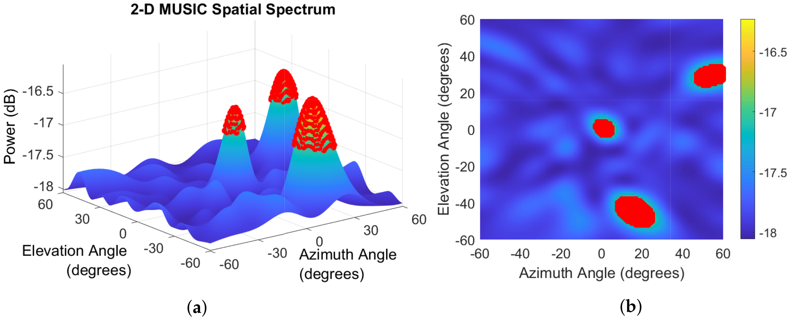
• A two-dimensional (2D) MUSIC algorithm estimator which will estimate the DOA in the range of −90° to 90° in both elevation and azimuth angles.
• A peak finder method to identify the peaks corresponding to the estimated DOAs in the spectrum plot generated from the 2D MUSIC estimator.

This simulation produces a covariance matrix that can be decomposed into magnitude and phase for training DL models. Figure 1 shows an example of a spatial spectrum produced by the simulation for three incoming signals with limited noise on an $8\times 8$ URA.

2.3. DL Framework

In mathematical optimization, a loss function or cost function is a function that maps an event or value of one or more variables onto a real number. An optimization problem seeks to minimize a loss function. The selection has been made that an objective function is equivalent to a loss or cost function. This, therefore, applies to the MUSIC algorithm function as it takes in combined signals and noise. It then outputs an estimation of DOA. In the case of the MUSIC algorithm, optimisation variables must be created of the combined signal and noise, such that it can be passed to an optimisation function of MUSIC with upper and lower bounds and a specified number of function evaluations.

DL approaches will be implemented using the Keras deep learning framework [21]. Artificial neural networks will be trained and validated with data generated from the simulation. As previously stated and shown in Figure 1, the simulation can handle multiple signals and resolve their directions of arrival successfully. However, in the following, the neural networks will only be tested against samples consisting of one signal. This will allow for more simple and rapid development of neural networks.

Approaches have been explored using the Adam optimiser [22] with standard learning rate, varying batch sizes and epochs, mean squared error (MSE) loss function, and rectified linear unit (ReLU) activation function (linear for final layer). Multi-layer perceptron (MLP), 1D convolutional neural networks (1D-CNN), and 2D-CNN have been developed. Initially, MLP was chosen as the most basic form of neural network to support rapid development, and to initially prove the validity of a deep learning approach. Following this, CNN’s were chosen to try and spot spatial features (peaks) within the array data by using convolutions of varying filters. We are faced with a MIMO regression problem because the aim is to learn from the values of magnitude and phase for each sample to predict two values for the DOA as azimuth and elevation angles. Figure 2, as an example, shows a representation of the structure of one of these neural networks (2D-CNN).

2.4. DL Approaches Description

The MLP is a type of feedforward NN that consists of multiple layers of interconnected neurons. Given an input vector $\mathbf{x}\in {\mathbb{R}}^d$, the output $\mathbf{y}\in {\mathbb{R}}^c$ of a MLP with L hidden layers can be computed as follows:

$$\begin{array}{cc}\hfill {\mathbf{h}}^{\left(1\right)}& ={\sigma }^{\left(1\right)}({\mathbf{W}}^{\left(1\right)}\mathbf{x}+{\mathbf{b}}^{\left(1\right)})\hfill \end{array}$$

(2)

$$\begin{array}{cc}\hfill {\mathbf{h}}^{\left(l\right)}& ={\sigma }^{\left(l\right)}({\mathbf{W}}^{\left(l\right)}{\mathbf{h}}^{(l-1)}+{\mathbf{b}}^{\left(l\right)})\mathrm{for}l=2,3,\dots ,L\hfill \end{array}$$

(3)

$$\begin{array}{cc}\hfill \mathbf{y}& =\mathrm{softmax}({\mathbf{W}}^{(L+1)}{\mathbf{h}}^{\left(L\right)}+{\mathbf{b}}^{(L+1)}),\hfill \end{array}$$

(4)

where ${\mathbf{W}}^{\left(l\right)}$ and ${\mathbf{b}}^{\left(l\right)}$ are the weight matrix and bias vector for the l-th layer, respectively. ${\sigma }^{\left(l\right)}$ is the activation function applied element-wise at the l-th layer, and softmax is the softmax function that converts the final layer output to a probability distribution.

The 1D-CNN is a type of convolutional neural network designed to process one-dimensional sequential data. Given an input sequence $\mathbf{x}\in {\mathbb{R}}^T$, the output $\mathbf{y}\in {\mathbb{R}}^c$ of a 1D-CNN with N filters of size F can be computed as follows:

$$y_i=\mathrm{ReLU}\left(\sum _{j=1}^F{w}_j·x_{i+j-1}+b\right)\mathrm{for}i=1,2,\dots ,T-F+1,$$

(5)

where $y_i$ is the i-th element of the output vector $\mathbf{y}$, $\mathrm{ReLU}\left(x\right)=$$max(0,x)$ is the rectified linear unit activation function, and $w_j$ and b are the filter weights and bias, respectively. Similarly, 2D-CNN can process two-dimensional data. Given an input $\mathbf{X}$$\in {\mathbb{R}}^{H\times W}$, the output feature map $\mathbf{Y}$$\in {\mathbb{R}}^{H^{\prime }\times W^{\prime }}$ of a 2D-CNN with N filters of size $F\times F$ can be computed as follows:

$$Y_{ij}=\mathrm{ReLU}\left(\sum _{m=1}^F\sum _{n=1}^F{w}_{mn}·X_{(i+m-1),(j+n-1)}+b\right)\mathrm{for}\left\{\begin{array}{c}i=1,2,\dots ,H^{\prime }-F+1\hfill \\ j=1,2,\dots ,W^{\prime }-F+1.\hfill \end{array}\right.$$

(6)

where $Y_{ij}$ is the element at position $(i,j)$ in the output feature map $\mathbf{Y}$, $\mathrm{ReLU}\left(x\right)=max(0,x)$ is the rectified linear unit activation function, and $w_{mn}$ and b are the filter weights and bias, respectively. MLP, 1D-CNN, and 2D exhibit distinct computational complexities. MLP is comparatively straightforward, comprising multiple fully connected layers.

2.5. Implementation

Keras is a DL application programming interface (API) written in Python, running on top of the ML platform TensorFlow [24]. It was developed with a focus on enabling fast experimentation. In this study, Keras was chosen for the deep learning approach because it effectively allowed for rapid experimentation against different approaches consisting of different neural network architectures. Keras offers consistent and simple APIs, such that it minimises the number of user actions required for the most common use cases [24,25].

Before the investigation into and development of the neural networks, a dataset for training and validation needed to be created. As previously stated, no dataset was available within the scope of this project. Therefore, all data for this section had to be generated by simulation. The designed simulation allows for data for any antenna array size. The data generation approach is as follows:

• Specify multiple noise power values. The models will need to be tested against signals in a spectrum of different noise conditions.
• For each noise power value, generate a signal for every angle 1° apart in the range of −60° to 60° in both azimuth and elevation angles.
• For the covariance matrix generated, take both the magnitude and phase values separately (as complex numbers). Absolute value and angle value are taken for magnitude and phase, respectively.
• Perform the conventional MUSIC algorithm estimation for each signal for later comparison. The MSE and mean absolute error (MAE) between estimates and true angles will be compared to the MSE and MAE achieved from the best neural networks. This will be the way to evaluate the success of the approach.
• Insert magnitude, phase and true angles into separate comma-separated value files inside the true angle file and save the MUSIC algorithm’s estimated values.

First, data are generated for a $2\times 2$ antenna array. This allows for the fastest experimentation with different neural network architectures and structures. Then, data were also generated for an $8\times 8$ antenna array. This produces the largest array size that could be feasibly used in training based on our hardware specifications. The implementation is shared as Supplementary Information. The computational complexity of a MLP depends on the number of layers and neurons in each layer. Training a MLP involves matrix multiplications and activation functions, resulting in a time complexity of $L\times N^2$, where L is the number of layers and N is the average number of neurons per layer. Despite their simplicity, MLPs might struggle to capture complex spatial relationships in data due to the absence of convolutions. In contrast, 1D-CNN introduces convolutional layers that operate along one dimension, typically suited for sequential data. The computational complexity of 1D-CNN is influenced by the kernel size, number of filters, and sequence length. Convolution operations in 1D-CNN involve a sliding window over the input sequence. This leads to a time complexity of approximately $F\times K\times N$, where F is the number of filters, K is the kernel size, and N is the sequence length. While 1D-CNN can effectively capture local patterns, its limitation to a single dimension can hinder its performance on data with intricate spatial structures. The 2D-CNN architecture extends convolution to two dimensions, making it well-suited for 2D data. The computational complexity of 2D-CNN is determined by kernel size, number of filters, image dimensions, and strides. Convolution operations in 2D-CNN involve sliding a filter over 2D space, resulting in a time complexity of roughly $F\times K^2\times H\times W$; H is the data height and W is the data width. The 2D-CNN excels at capturing spatial hierarchies and patterns within data, making it a staple in field-of-view tasks.

2.6. Testing Keras DL

The approach to testing Keras DL methods is detailed below to ensure ease in repeatability of the experimentation:

• For data preprocessing methods (e.g., dimensionality reduction and splitting training and test sets), provide mock data to the methods and make assertions on the properties of the returned data. For example, assert that the correct shape and size of the data are returned, or that the correct split sizes on the data are returned.
• For neural network generation methods (e.g., generating MLP, 1D-CNN, combining models, etc.) test that parameterised creation of networks works as expected. Create a standard neural network from methods and then create an equivalent model using the Keras functional API in the test. Finally, assert that the output shapes of the layers and the number of layers are equal.
• For testing metrics methods (e.g., generating MUSIC metrics) test that metric values are returned as expected. For example, mock output data and calculate MSE and MAE, and calculate the number of out-of-range values (NaN). Finally, assert that these values are the same as those returned from the metrics methods.

Only the methods for generating the DL approaches will be tested. The Jupyter Notebook will include multiple implementations of these data generation methods, but they themselves do not require testing. Testing them would involve extensive modifications and would only verify the usage of already tested methods. Furthermore, the continuous regression outputs of these methods make their feasibility for testing impractical.

3. Simulation Results and System Evaluation

In this Section, the results from each of the attempted DL approaches will be evaluated. Because a large amount of experimentation with different structures was attempted only the final results from each design are included here. To limit the workload, an optimum NN has been determined using a set of standard parameters and activation functions (learning rate: 0.001, activation function: ReLU, batch size: 32). Each approach has been trained and tested against three datasets generated from the simulation. These are:

• Data generated from a $2\times 2$ URA. This array generates raw data that can contain complex patterns and information related to signal sources, interference, and spatial relationships.
• The same $2\times 2$ URA data, this time with principal component analysis (PCA) dimension reduction [26] has been applied to it. PCA works by transforming the original dataset into a new set of orthogonal variables called principal components. These components capture the most significant variance present in the data. By applying PCA to the $2\times 2$ URA data, one aims to reduce the complexity of the dataset while retaining the most critical information. PCA can potentially enhance the SNR, suppress noise, and highlight important patterns, which may lead to more accurate and robust analysis outcomes. However, there is a trade-off between the reduction in dimensionality and the retention of information. It is important to carefully examine how much variance is retained after dimension reduction and whether the reduction in complexity leads to a significant loss of critical information.
• Data generated from an $8\times 8$ URA with applying PCA. Expanding upon the exploration of URAs and PCA, we now consider a larger array configuration. The data generated from an $8\times 8$ URA represents a more complex and richer dataset compared to the previous $2\times 2$ URA scenario, potentially capturing a more diverse range of signal sources and spatial patterns. The goal remains consistent: to determine whether the reduction in dimensionality through PCA enhances or diminishes the analytical outcomes, and to strike a balance between complexity reduction and information preservation.

It should be noted here that the studied URA architectures can be scaled to include a larger number of antenna elements without loss of generality. However, such a choice will require more advanced computing resources due to the increased computational complexity. In this work, an HP Inc. desktop machine (intel-i7 3.4 GHz with 32 GB RAM with SSD) was used in the studied scenarios. Before presenting the final results, here is a summary of the findings of the initial tests:

• The combination approach provides better accuracy than any approach against only magnitude or phase.
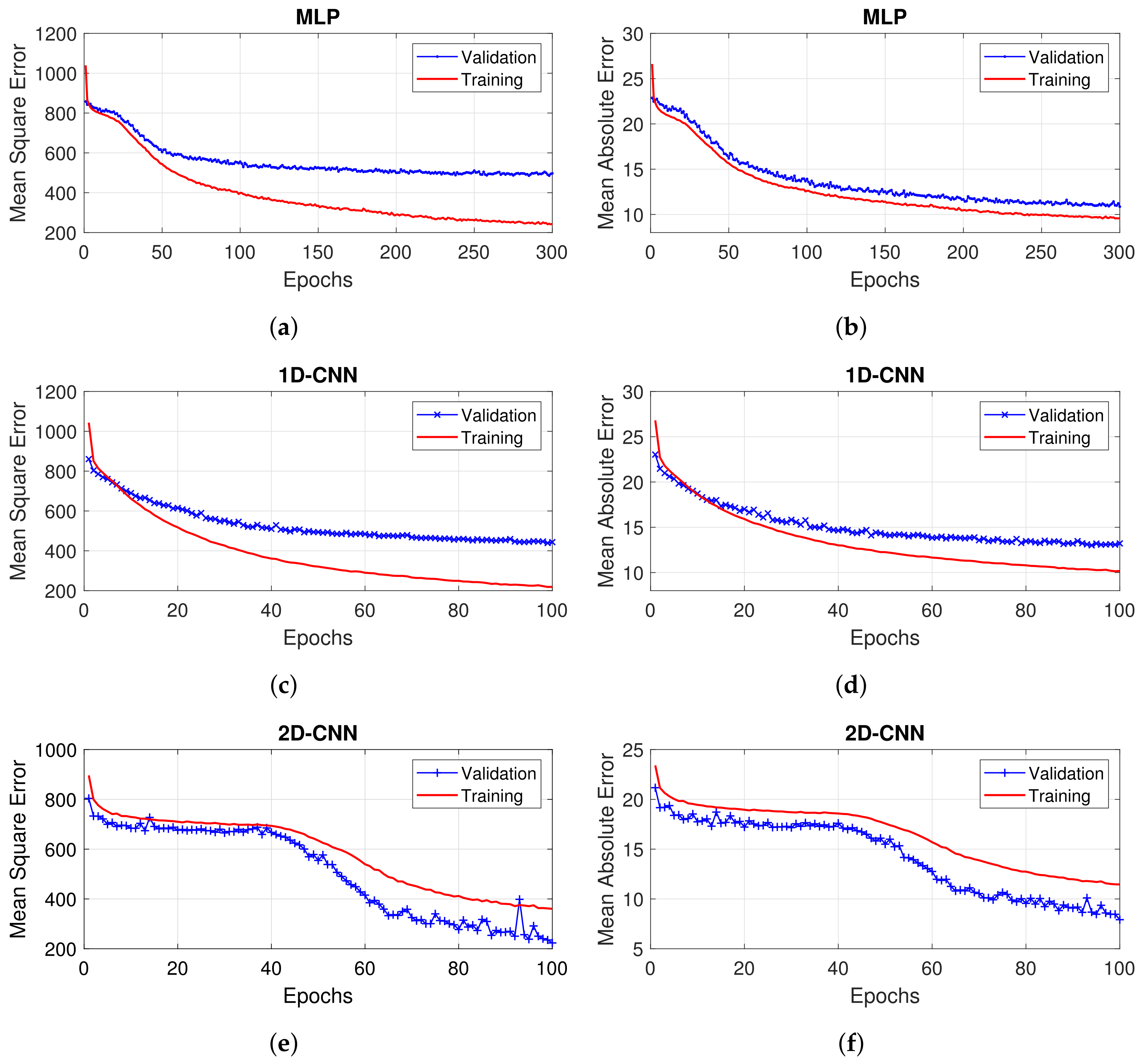
• The MLP approach works better against dimensionally reduced data. This is expected as it allows for a simpler neural network design with fewer connections which also helps to reduce overfitting.
• The 1D-CNN approach works better against non-reduced data. This makes sense as a CNN works by extracting features that may be reduced or distorted when PCA is performed.
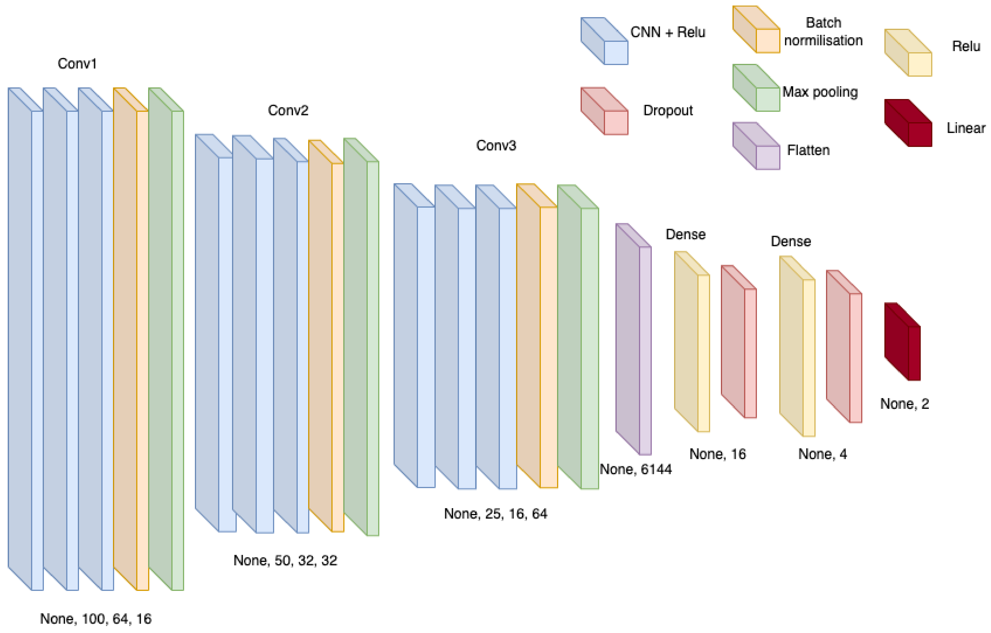
• The best results are generated from the 2D-CNN approach. This is also expected as this approach allows for the structure of the originally generated data (two dimensions) to be maintained and thus features can be more accurately defined. However, this approach can only be achieved against the non-dimensionally reduced data in our current hardware.

In

Table 1. Outputs of the best simulation results for different DL approaches compared to the pure MUSIC algorithm (all MSE and MAE figures are rounded off to two decimal places for comparison consistency).

Approach	Dataset	MSE	MAE
MLP-based	$8\times 8$ URA with PCA	497.03	10.86
1D-CNN-based	$8\times 8$ URA with PCA	443.59	13.21
MUSIC	$8\times 8$ URA with PCA	1375.57	21.15
2D-CNN-based	$2\times 2$ URA	223.35	7.92
MUSIC	$2\times 2$ URA	75.58	5.15

, the final simulation results for each DL approach is compared with the pure MUSIC algorithm. Moreover, the corresponding MSE and MAE graphs are shown in Figure 3. As can be seen, the graphs show a large decrease in the MAE and the MSE across the epochs, indicating that the training was successful. The models are also not overfitting as the validation curves are keeping in line with the training curves shown for each approach in Figure 3. In the case of 2D-CNN, the validation values are approaching that of the original MUSIC algorithm. It is important to note that not every approach has outperformed the conventional MUSIC algorithm, however, the closeness to the original algorithm, in this case, proves the validity of the DL model replacement.

A major advancement of the proposed DL approach, when compared with the conventional MUSIC algorithm, relates to its extended capability in predicting a broader range of angles. It is noteworthy that the conventional MUSIC algorithm, when confronted with an angle falling outside the range of −90° to 90°, yields no prediction, leading to a return of “NaN”. In contrast, the DL approach exhibits proficiency in handling such angles. Moreover, it is imperative to monitor and account for the instances in which “NaN” values arise, as angles may indeed extend beyond the −90° to 90° range due to the pervasive impact of heightened noise power. This oversight is an integral aspect of data processing and analysis, underpinning the reliability of the DL approach. For example, the conventional MUSIC algorithm encounters challenges when predicting angles within the scope of high noise power conditions for a $2\times 2$ URA. Specifically, scenarios such as [−55°, 23°] prove problematic for the conventional MUSIC algorithm to resolve, yet the DL approach adeptly overcomes this limitation, successfully determining the DoA as [−23.98°, 29.89°].

Upon examination of the data generated from the $2\times 2$ URA and subsequent results (Figure 3), a notable observation emerges: the conventional MUSIC approach grapples with the resolution of a substantial count of 211 values within the entire validation set comprising 46,852 samples. Conversely, the 2D-CNN effectively resolves all of these challenging samples with a MSE of 407.94 and a MAE of 12.45. It is prudent to acknowledge that these error metrics register values higher than the overall average for the validation set, which is to be anticipated. The rationale for this deviation is that the noise values accompanying these samples are comparatively large and sufficiently substantial to prevent the conventional MUSIC algorithm’s ability to provide accurate estimates. This contextual understanding underscores the rationale behind the comparatively increased error margin exhibited by the DL approach in this specific subset of the validation dataset. While this subset represents a fraction of the complete validation set, it undeniably signifies a promising stride towards enhanced performance. Furthermore, it is worth highlighting that the DL approach’s introduction into the DoA estimation is an original avenue of inquiry. This distinctive exploration establishes the proposed approach as a self-contained and innovative investigation, warranting an independent evaluation without direct comparison to other studies within the existing literature. Moreover, it is worth mentioning that the optimal parameters associated with the approach are not presented, and this omission stems from the parameters’ inherent hardware-specific nature, thus recognizing the distinctiveness of the proposed approach associated with hardware configurations.

4. Conclusions and Future Works

In this paper, a DL approach for DOA estimation was proposed and implemented. First, a framework for the simulations was defined in such a way that signals can be generated that, when combined with noise, produce a covariance matrix that can be decomposed and used to train a DL method. The validity of this framework was shown in the relevant criteria. The simulation framework also provides a benchmark of a standard DOA estimation algorithm (in this paper MUSIC) against which the results of the designed DL approach can be compared. Then, several DL methods were explored with key design decisions for each of the identified cases. Finally, systems approaching the accuracy of the MUSIC algorithm for resolving a noisy signal were obtained, and in some better detection ranges even outperformed the conventional MUSIC algorithm.

Although the results of this paper are considered promising, the implemented approach still faces the following limitations, which will be considered for further development in future works:

• Based on the experimental data, the results will be further validated.
• The DL approach has currently only been tested on a maximum antenna size of $8\times 8$ antennas when a real-world computation for a massive MIMO system would tend to be $64\times 64$. This was due to the limited hardware capabilities available for this work. Moreover, analysis around computational time needs further study.
• The DL approach currently only makes predictions for single signal data. However, the MUSIC algorithm can resolve high numbers of signals with high accuracy. It would therefore be necessary that the DL models be adapted to allow for multiple signal classifications.

References

1. Saleem, A.; Cui, H.; He, Y.; Boag, A. Channel propagation characteristics for massive multiple-input/multiple-output systems in a tunnel environment [measurements corner]. IEEE Antennas Propag. Mag. 2022, 64, 126–142. [Google Scholar] [CrossRef]
2. Catreux, S.; Driessen, P.F.; Greenstein, L.J. Data throughputs using multiple-input multiple-output (MIMO) techniques in a noise-limited cellular environment. IEEE Trans. Wirel. Commun. 2002, 1, 226–235. [Google Scholar] [CrossRef]
3. Chen, J.; Li, S.; Tao, J.; Fu, S.; Sobelman, G.E. Wireless beam modulation: An energy-and spectrum-efficient communication technology for future massive IoT systems. IEEE Wirel. Commun. 2020, 27, 60–66. [Google Scholar] [CrossRef]
4. Imoize, A.L.; Obakhena, H.I.; Anyasi, F.I.; Sur, S.N. A Review of Energy Efficiency and Power Control Schemes in Ultra-Dense Cell-Free Massive MIMO Systems for Sustainable 6G Wireless Communication. Sustainability 2022, 14, 11100. [Google Scholar] [CrossRef]
5. Byreddy, A.R.; Logashanmugam, E. Energy and spectral efficiency improvement using improved shark smell-coyote optimization for massive MIMO system. Int. J. Commun. Syst. 2023, 36, e5381. [Google Scholar] [CrossRef]
6. Liu, Y.; Dong, N.; Zhang, X.; Zhao, X.; Zhang, Y.; Qiu, T. DOA Estimation for Massive MIMO Systems with Unknown Mutual Coupling Based on Block Sparse Bayesian Learning. Sensors 2022, 22, 8634. [Google Scholar] [CrossRef] [PubMed]
7. Aquino, S.; Vairavel, G. A Review of Direction of Arrival Estimation Techniques in Massive MIMO 5G Wireless Communication Systems. In Proceedings of the Fourth International Conference on Communication, Computing and Electronics Systems: ICCCES 2022, Coimbatore, India, 15–16 September 2022; Springer: Berlin/Heidelberg, Germany, 2023; pp. 15–34. [Google Scholar]
8. Gu, J.F.; Zhu, W.P.; Swamy, M. Joint 2-D DOA estimation via sparse L-shaped array. IEEE Trans. Signal Process. 2015, 63, 1171–1182. [Google Scholar] [CrossRef]
9. Guo, M.; Chen, T.; Wang, B. An improved DOA estimation approach using coarray interpolation and matrix denoising. Sensors 2017, 17, 1140. [Google Scholar] [CrossRef] [PubMed]
10. Shi, Z.; He, Q.; Liu, Y. Accelerating parallel Jacobi method for matrix eigenvalue computation in DOA estimation algorithm. IEEE Trans. Veh. Technol. 2020, 69, 6275–6285. [Google Scholar] [CrossRef]
11. Ge, S.; Li, K.; Rum, S.N.B.M. Deep learning approach in DOA estimation: A systematic literature review. Mob. Inf. Syst. 2021, 2021, 6392875. [Google Scholar] [CrossRef]
12. Molaei, A.M.; Del Hougne, P.; Fusco, V.; Yurduseven, O. Numerical-Analytical Study of Performance of Mixed-Order Statistics Algorithm for Joint Estimation of DOA, Range and Backscatter Coefficient in a MIMO Structure. In Proceedings of the 2022 23rd International Radar Symposium (IRS), Gdansk, Poland, 12–14 September 2022; IEEE: New York, NY, USA, 2022; pp. 396–401. [Google Scholar]
13. Shaikh, S.A.; Tonello, A.M. DoA estimation in EM lens assisted massive antenna system using subsets based antenna selection and high resolution algorithms. Radioengineering 2018, 27, 159–169. [Google Scholar] [CrossRef]
14. Yadav, S.K.; George, N.V. Coarray MUSIC-group delay: High-resolution source localization using non-uniform arrays. IEEE Trans. Veh. Technol. 2021, 70, 9597–9601. [Google Scholar] [CrossRef]
15. Merkofer, J.P.; Revach, G.; Shlezinger, N.; Routtenberg, T.; van Sloun, R.J. DA-MUSIC: Data-Driven DoA Estimation via Deep Augmented MUSIC Algorithm. In Proceedings of the ICASSP 2022—2022 IEEE International Conference on Acoustics, Speech and Signal Processing (ICASSP), Toronto, ON, Canada, 6–11 June 2021. [Google Scholar]
16. Jaafer, Z.; Goli, S.; Elameer, A.S. Best performance analysis of doa estimation algorithms. In Proceedings of the 2018 1st Annual International Conference on Information and Sciences (AiCIS), Dhaka, Bangladesh, 19–21 December 2020; IEEE: New York, NY, USA, 2018; pp. 235–239. [Google Scholar]
17. Huang, Q.; Lu, N. Optimized Real-Time MUSIC Algorithm With CPU-GPU Architecture. IEEE Access 2021, 9, 54067–54077. [Google Scholar] [CrossRef]
18. Moein, M.M.; Saradar, A.; Rahmati, K.; Mousavinejad, S.H.G.; Bristow, J.; Aramali, V.; Karakouzian, M. Predictive models for concrete properties using machine learning and deep learning approaches: A review. J. Build. Eng. 2022, 63, 105444. [Google Scholar] [CrossRef]
19. Ma, R. Wideband, Direction of Arrival Estimation Using Small-Aperture Antenna Arrays; The University of Wisconsin-Madison: Madison, WI, USA, 2020. [Google Scholar]
20. Xu, K.; Quan, Y.; Bie, B.; Xing, M.; Nie, W.; Hanyu, E. Fast direction of arrival estimation for uniform circular arrays with a virtual signal subspace. IEEE Trans. Aerosp. Electron. Syst. 2021, 57, 1731–1741. [Google Scholar] [CrossRef]
21. Moolayil, J.; Moolayil, J. An introduction to deep learning and keras. In Learn Keras for Deep Neural Networks: A Fast-Track Approach to Modern Deep Learning with Python; Apress: Berkeley, CA, USA, 2019; pp. 1–16. [Google Scholar]
22. Zhang, Z. Improved adam optimizer for deep neural networks. In Proceedings of the 2018 IEEE/ACM 26th International Symposium on Quality of Service (IWQoS), Banff, AB, Canada, 4–6 June 2018; IEEE: New York, NY, USA, 2018; pp. 1–2. [Google Scholar]
23. Lecun, Y.; Bottou, L.; Bengio, Y.; Haffner, P. Gradient-based learning applied to document recognition. Proc. IEEE 1998, 86, 2278–2324. [Google Scholar] [CrossRef]
24. About Keras. Available online: https://keras.io/about/ (accessed on 1 July 2023).
25. Why Choose Keras? Available online: https://keras.io/why_keras/ (accessed on 1 July 2023).
26. Hasan, B.M.S.; Abdulazeez, A.M. A review of principal component analysis algorithm for dimensionality reduction. J. Soft Comput. Data Min. 2021, 2, 20–30. [Google Scholar]
Figure 1. An example of the pseudospectrum produced by the simulator for three noisy signals with azimuth and elevation DOAs of ( θ , ϕ ) =(17°, −45°), (0°, 0°), and (55°, 30°) with an 8 × 8 URA; (a) 3D view, (b) 2D view when red indicate the peaks.
Electronics 12 03505 g001
Figure 2. A concept example of a 2D-CNN structure, in this case for a two-by-two antenna array with initial shape corresponding to the array size generated by these elements [23].
Electronics 12 03505 g002
Figure 3. Graphs of accuracy across epochs. (a) MSE and (b) MAE for MLP-based 8 × 8 URA with PCA. (c) MSE and (d) MAE for 1D-CNN-based 8 × 8 URA with PCA. (e) MSE and (f) MAE for 2D-CNN-based, 2 × 2 URA.
Electronics 12 03505 g003