Simulation-Based Headway Optimization for the Bangkok Airport Railway System under Uncertainty

Abstract

The ever-increasing demand for intercity travel, as well as competition among all modes of transportation, is an unavoidable reality that today’s urban rail transit system must deal with. To meet this problem, urban railway companies must try to make better use of their existing plans and resources. Analytical approaches or simulation modeling can be used to develop or change a rail schedule to reflect the appropriate passenger demand. However, in the case of complex railway networks with several interlocking zones, analytical methods frequently have drawbacks. The goal of this article is to create a new simulation-based optimization model for the Bangkok railway system that takes into account the real assumptions and requirements in the railway system, such as uncertainty. The common particle swarm optimization (PSO) technique is combined with the developed simulation model to optimize the headways for each period in each day. Two different objective functions are incorporated into the models to consider both customer satisfaction by reducing the average waiting time and railway management satisfaction by reducing needed energy usage (e.g., reducing operating trains). The results obtained using a real dataset from the Bangkok railway system demonstrate that the simulation-based optimization approach for robust train service timetable scheduling, which incorporates both passenger waiting times and the number of operating trains as equally important objectives, successfully achieved an average waiting time of 11.02 min (with a standard deviation of 1.65 min) across all time intervals.

1. Introduction

1.1. Background of Study and Motivations

As the distance between people’s homes, centers, and services such as education, entertainment, shopping, and health care has expanded, the necessity for everyday travel has increased, and serving this high volume of travel requires appropriate transportation platforms. The disparity between road network capacity and trip volume necessitates the development of public transportation networks as an alternative to private vehicles. From the standpoint of macroeconomic management, urban rail network infrastructure appears to be more cost-effective in terms of issues that could have a long-term impact on the country’s resources or result in an increase in public spending. Taking the example of a subway train, it is 4.23 times more efficient than the most complete car with the lowest fuel usage [1]. Over the years, as traffic volumes and pollution emissions have increased, a greater emphasis has been placed on the development of more environmentally aware transportation systems. A direct result is the pursuit of more efficient energy management. In railways, this improved management may be desired first and probably most importantly during the planning phase, which is when timetables are constructed [2]. To be more specific, it is necessary to estimate the train running times between stations during the planning phase to compute train schedules. It is also essential to compute the energy-optimal train trajectories offline before communicating them to the driver in the form of a roadmap, which he or she must adhere to by following the timetable and predefined running times [3]. To maintain a high level of service during operations, railway timetables must provide competitive travel times while also being able to withstand delays, perturbations, and variations in operating conditions without losing functionality. Several performance indicators related to individual train paths (running and dwelling), dependencies between train paths (headways, turning, transferring, and so on), and integrated train paths are used in the design of such a timetable (corridors and networks). Infrastructure occupancy, timetable stability, feasibility, robustness, and resilience are some of the performance indicators that are measured. How these performance indicators are dealt with can be used to determine the overall quality of the timetable design process [4]. Due to the growth of its metropolitan areas, Bangkok is the top city in terms of worst traffic congestion in the world. Bangkok demands an accessible railway transportation system, which is the priority for improving the traffic congestion problem, leading to lower air and noise pollution. In 2021, the Bangkok railway system carried a total of approximately 180 million passengers, which averages to around 500,000 passengers per day [5]. Therefore, Thailand’s government has committed to investing in and expanding public transport, especially the Bangkok railway system, and hence the optimal management of transportation that is flexible enough to deliver economical services to the large population while considering Bangkok’s city infrastructure. To ensure the adaption of Bangkok railway transportation by a citizen, much needs to be done to enhance the quality in terms of service, resource optimization, access, and availability, which can be accomplished by integrating intelligent technology. The optimization and simulation techniques will help in developing and proposing a model for simulating the supportive approach for upgrading the railway system to an intelligent transportation system soon. In the current study, we develop a new simulation-based multi-objective optimization model for the optimization of headway in the Bangkok railway system under uncertainty, which is then implemented in practice. The emphasis is on developing a simulation model which is then used as a foundation for optimizing the headway. In other words, a simulation model is used to evaluate solutions generated by the PSO algorithm. The airport rail link (ARL) is the one partner of this research for data acquisition which we researched and applied practically to solve this problem. Some part of this research objective is from the focus problems that we collected and observed in the Bangkok railway system, especially for the ARL, providing data for observation of the focus problems in train headway optimization, as we mention in Section 2.

1.2. Related Works

The problem of scheduling timetables has been approached in a variety of ways in the literature with or without consideration of energy and involving one or more objectives (see [6,7]). However, the application of evolutionary computation techniques to a real-world complex train schedule multi-objective problem is still an open and challenging issue that requires further investigation. Evolutionary computation techniques such as PSO, the genetic algorithm (GA), and differential evolution (DE) have been used widely to solve various single- and multi-objective optimization and learning problems. It was demonstrated in [8] that evolutionary algorithms could be applied to a real-world complex train schedule multi-objective problem by considering a GA and PSO and DE algorithms to solve the train schedule optimization. They also compared the performances of these three algorithms based on multi-objective train scheduling problems, and they found that the DE approach produced the best simulation results out of the three evaluation algorithms. With a particular emphasis on passenger railway services in Europe, the authors of [9] presented an extensive survey on practical applications and combinatorial optimization models for railway timetable optimization, as well as methods for improving robust timetabling models. A comprehensive study of multi-objective evolutionary algorithms and the application of multi-objective evolutionary algorithms to a variety of optimization issues was provided in [10]. The authors of [11] provided an overview and the characteristics of multi-objective evolutionary algorithms, as well as an analysis of the strengths and weaknesses of various evolutionary methods for multi-objective optimization algorithms when their overall simulation results showed that not one of the methods was the most superior when all aspects of the performance measures were taken into consideration.

Table 1. Research classification of simulation-based optimization in railway systems.

Study	Objective	Optimization	Solution Approach
25	Reducing passenger waiting time and energy consumption.	Timetable	A fuzzy multi-objective optimization algorithm
26	Find the most appropriate train target speed profile to minimize energy usage and enhance train punctuality.	Train speed profiles	Enhanced brute force, ant colony optimization, and GA
27	Minimize the waiting time of passengers and operation costs.	Timetable	Lagrangian duality theory
28	Average passenger travel time and rate of carriage fullness.	Headway	Response surface methodology (RSM)
29	Minimize headway by considering trip time.	Headway	PSO algorithm
30	Energy saving and reducing passenger waiting time.	Timetable	A Lagrangain relaxation-based and heuristic algorithm
31	Minimize the total tractive energy consumption.	Timetable and speed profile	Simulation-based genetic algorithm incorporated
32	Minimize the total passenger travel time, which consists of waiting and riding time	Timetable	The spatial branch and bound algorithm
This study	1. Minimize average waiting time (customer satisfaction).2. Minimize operation cost (railway management satisfaction).	Timetable (headways for each operation period per day)	Develop Python-based simulation and optimize using PSO

shows five recent studies which are close to the scope of the current work and in the same area for simulation-based optimizing headway and train schedules in railway systems. As for the present management of the railway network downtown, economical solutions to satisfy the growing demand for transportation services, especially in an existing network with very limited financial resources and management for infrastructure development [12], the regular concept of the existing railway network management for economical services and satisfaction of passengers depends on the approach to timetable management, speed operation, train headway, average waiting time and traveling time of the passenger, etc. [13].

There are a few works which used a microscopic synchronous railway simulation modeling program called “Opentrack simulation” to evaluate the performance of the simulation for the improvement of the railway system in Thailand. Because of the expansion of the Sukhumvit Green Line, the number of passengers has tended to increase. The research in [14] proposed full-loop operation and two different short-term operations for solving the unbalanced passenger usage between the existing and extended lines from Bearing to Kheha-Samutprakarn. However, this also has limitations for actual usage, and delays may occur at the turnback point. A new extended service concept has been introduced in Bangkok’s operational railway system, the eastern high-speed train, to connect three airports. Many different train service types are used the same rail route. With the mixed-service operations and train configurations, it is a challenge to plan the timetable. This study constructs feasible timetables for mixed-service operations, with the airport rail link (ARL) and high-speed trains running on the same line.

1.3. Main Contributions

In the current paper, our contributions to the modeling and simulation of Bangkok rail transit systems include the following:

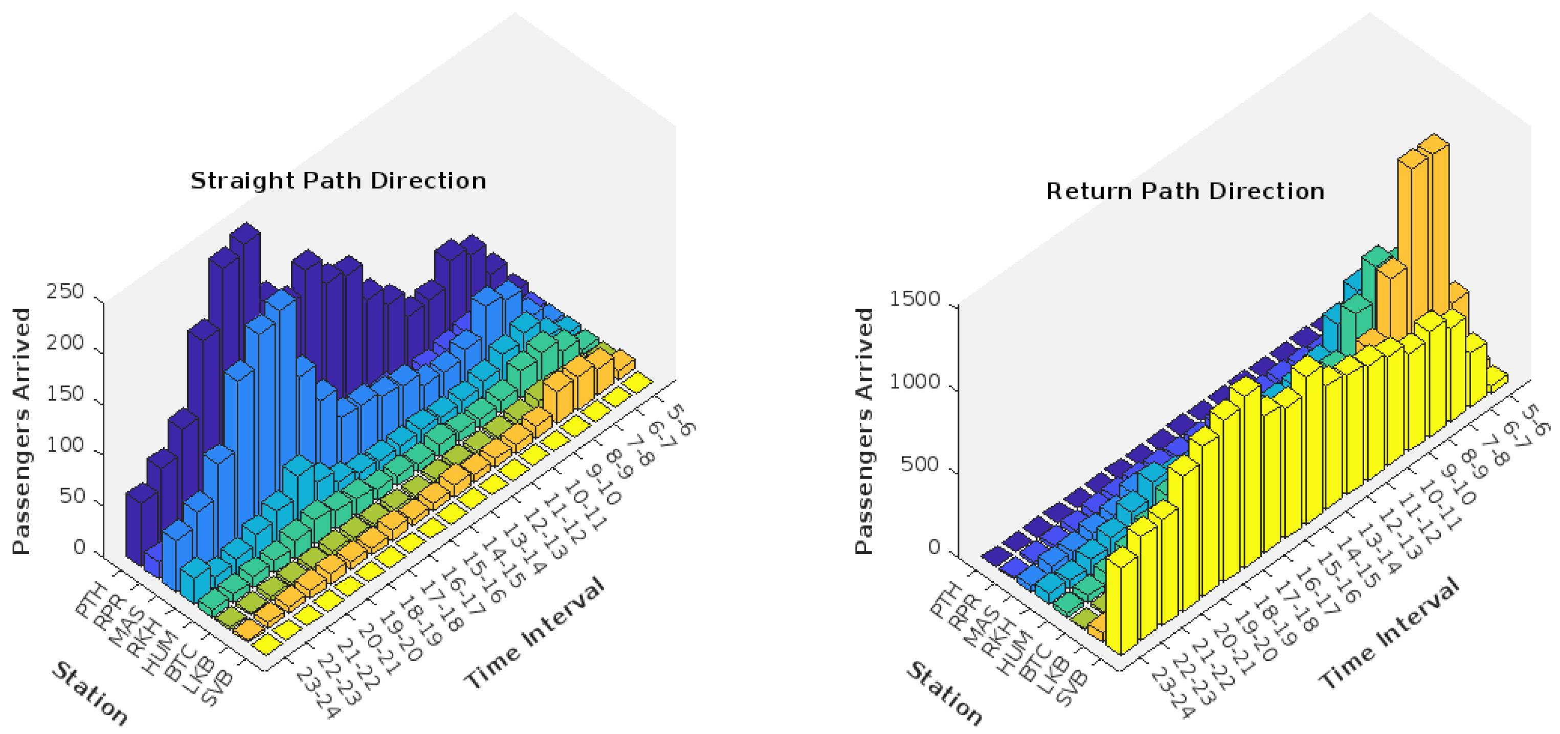
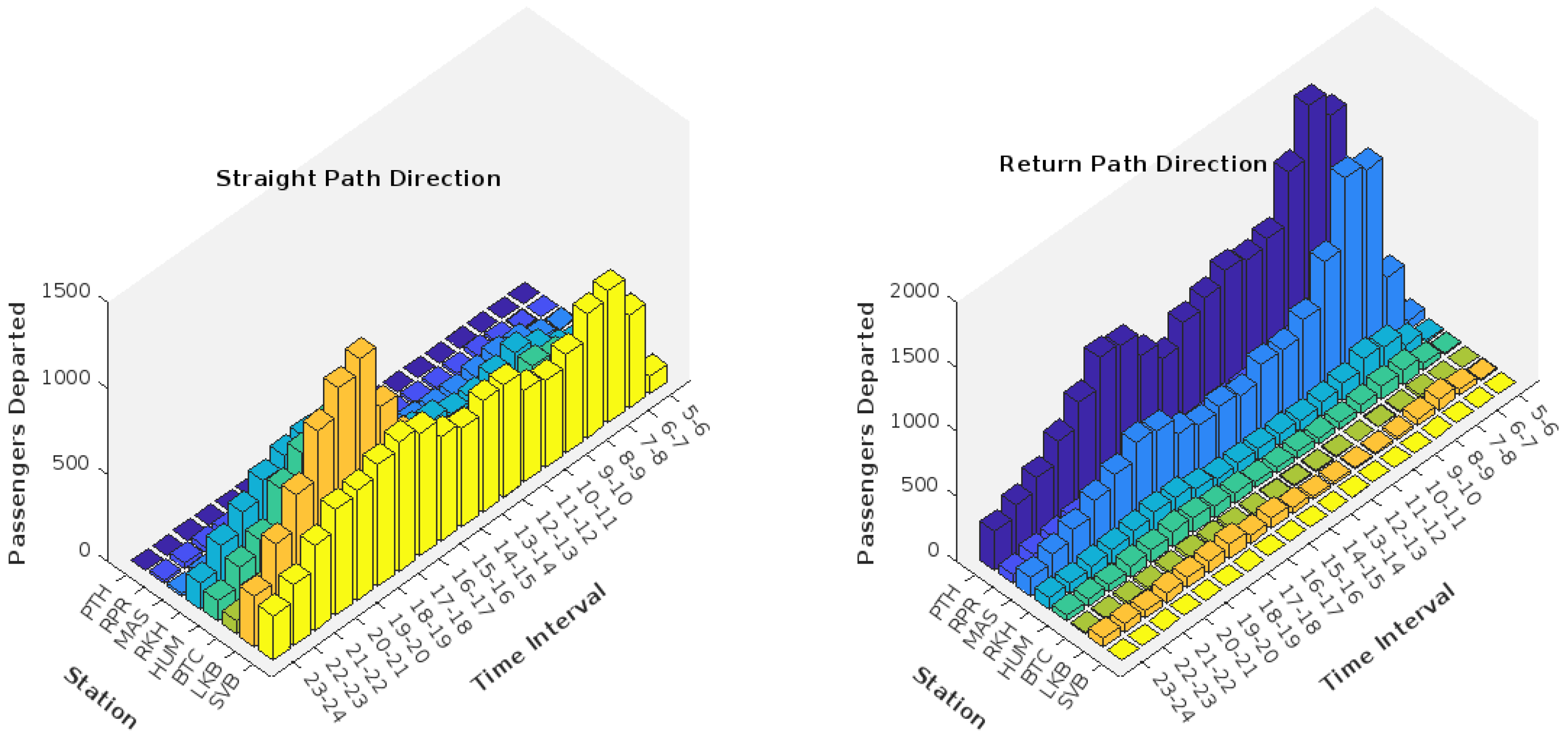
• Real data, including arrival and departure rates, were collected for one month (from 1 to 28 February 2021) from the control office of the railway. The collected data were gathered separately for weekdays and weekends.
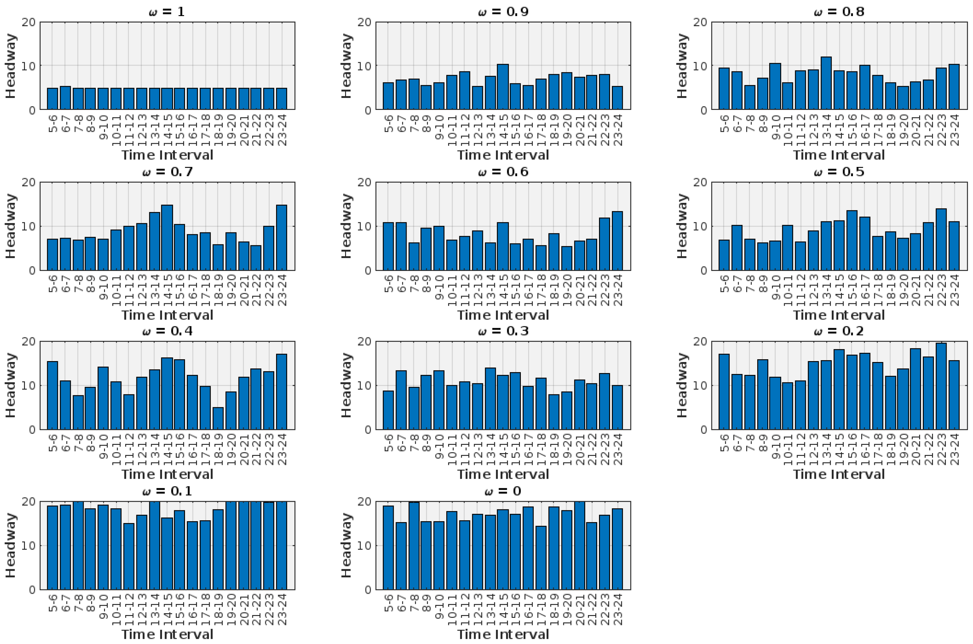
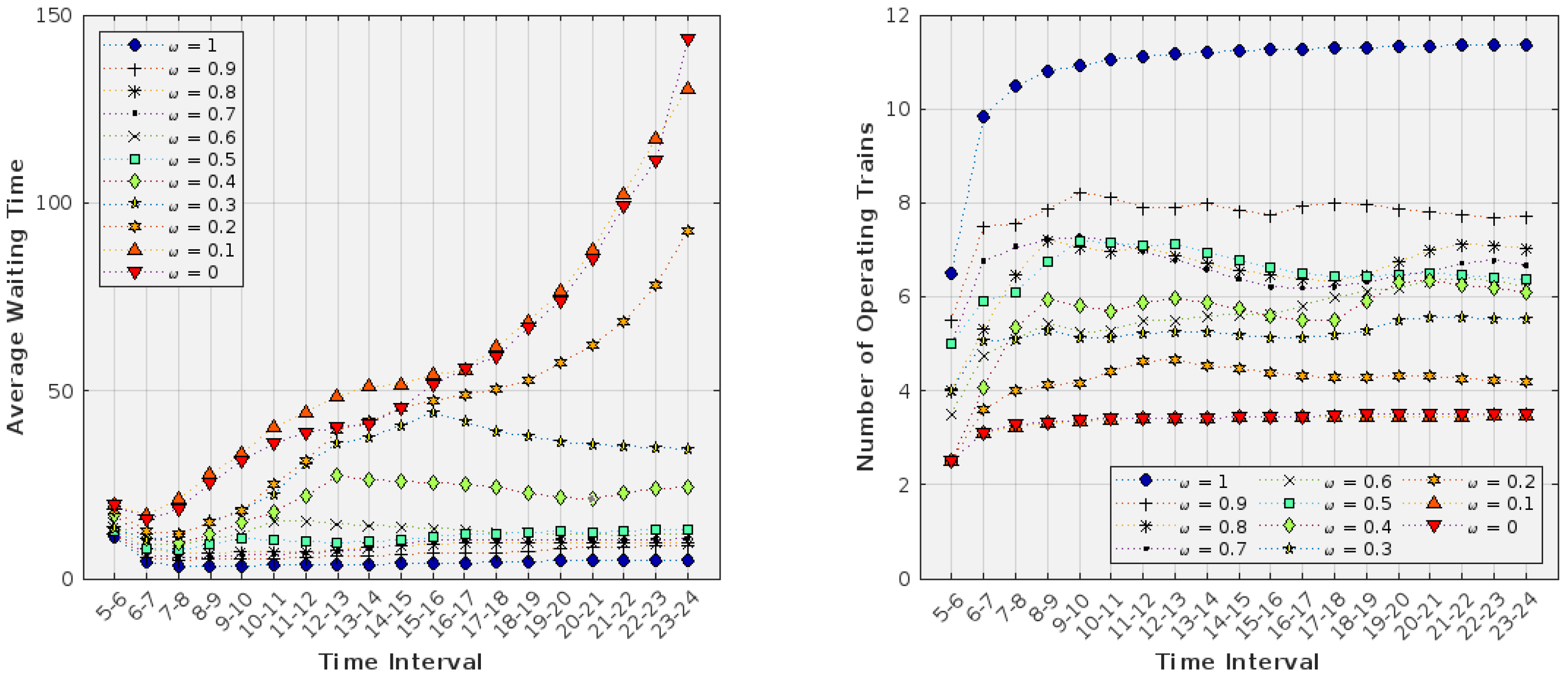
• Two conflicting objective functions are considered in the model: passenger satisfaction (which is maximized by minimizing the average wait time) and railway operating system costs (minimizing the required number of operating trains). When the wight scale $\omega$, is close to one, smaller headways are obtained for each time interval, and when $\omega$ is close to zero, the headways become larger for all time intervals.
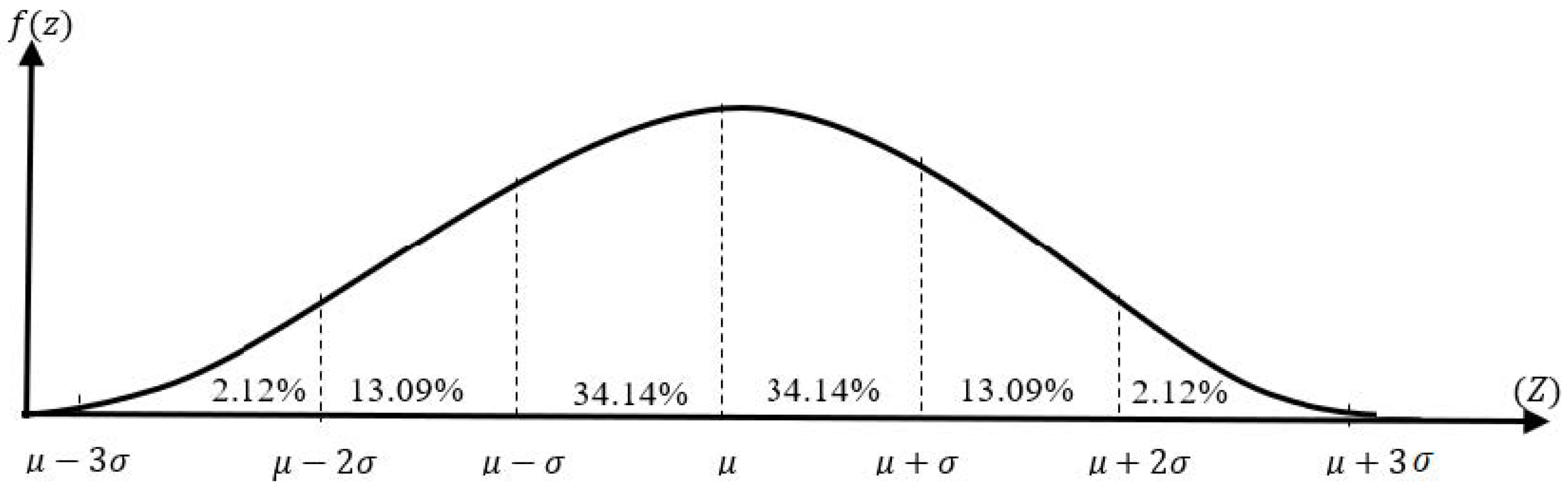
• Uncertainty in arrival rate is taken into account to investigate the sensitivity of the obtained solutions against variability in the arrival rate. The effect of uncertainty on the average wait time for three different uncertainty scenarios due to variability in arrival rates on different days of the month is given in Section 5. The results in Section 5 show that with the average arrival rate with a fixed coefficient of standard deviation, the greater the number of passengers who arrived at the stations, the greater average waiting time.
• Computation of the Pareto front with alternative optimal train headways is attended to with a multi-objective PSO algorithm using the developed simulation model.
• Comprehensive results are developed and discussed to assist train operators of the Bangkok railway system in determining the optimal real-time train schedules. A maximum of 13.21 min and minimum of 7.60 min with a standard deviation of 1.65 min for the average waiting time for all time intervals, including crowd peak times, are obtained.

The following sections comprise the remainder of the paper. Section 2 describes the practical problem of the Bangkok railway system in detail. Section 3 presents a simulation-based multi-objective optimization model of an uncertain railway system. Section 4 presents the obtained results using the proposed model, followed by Section 5, which concludes the paper.

2. Problem Statement

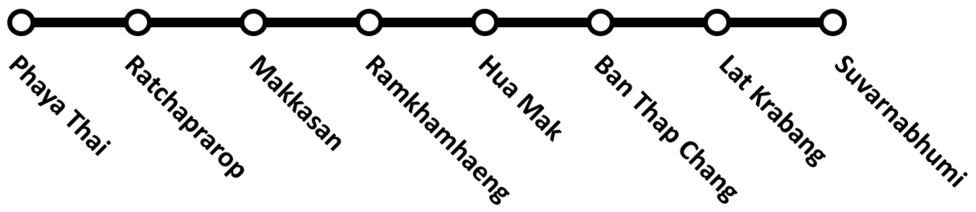
2.1. Bangkok Railway System

According to the operation characteristics of the Bangkok railway system, we develop the simulation model described in this section. As for the stated problem and limitation of existing management of the Bangkok railway system, the Bangkok Mass Transit System (BTS), metropolitan rapid transit (MRT), and ARL are the three main downtown transportation systems used by Bangkok citizens. To observe the problem and solution management recommendations, an optimizer and simulation tools were proposed to deliver economical services and adapt to the number of passengers. We repurposed the model for general use in the Bangkok railway system. However, in this paper, the data and study were limited to the ARL for implementation, which was supported by data from the airport rail link of the State Railway of Thailand. The ARL is a Bangkok train service for passengers between Bangkok downtown and the Bangkok-Suvarnabhumi Airport. The ARL was established and began operations in 2010. Initially, the train service had two types of operational train services. The train services consisted of both express services and the city line. However, the express service was canceled due to the lower expected number of passengers. At present, the ARL operates nine trains on the city line with the Siemens Desiro UK class 360/2 train. The nine trains consist of two types of trains: the city line train (5 trains with a maximum capacity of 745 passengers) and the modified express train (4 trains with an approximate maximum capacity of 740 passengers). The modified express service is expected to be upgraded to a maximum approximate capacity of 1000 passengers in the near future. The operation’s approximate average train speed and maximum train speed are 64 and 160 km/h, respectively. The ARL railway structure is 28.6 km long with 8 stations. The stations run between Suvarnabhumi Airport (A1-SVB), Lad Krabang (A2-LKB), Ban Thap Chang (A3-BTC), Hua Mark (A4-HUM), Ramkhamhaeng (A5-RKH), Makkasan (A6-MAS), Ratchaprarop (A7-RPR), and Phayathai (A8-PTH). The distance between each station (PTH–RPH, RPR–MAS, MAS–RKH, RKH–HUM, HUM–BTC, BTC–LKB, and LKB–SVB) is 0.8, 2.2, 4, 5, 5, 6, and 5 km, respectively. The schematic of the Bangkok railway system in one direction is shown in Figure 1.

2.2. Assumption and Requirements

With the improvement to railway operation, management needs the technology for testing, designing, and evaluating the most capable effects for the service provided. To reduce the imports of technology and promote our own country’s production, the country’s development of railway system technology needs to be studied and developed by ourselves. Consequently, research and development of the railway networks in Thailand is the key point to obtaining the maximum efficiency of management, including the consideration of the passengers serviced rate, which is compared to the service use time. Train system management requires a system or software for station and timetable operation management. Train operators could be carry out further development and adjustments by themselves in the future. Therefore, the purpose of this research is to create a prototype of open-source application software with simulation-based headway optimization to raise the management efficiency of the Thai railway network in the future. This open-source simulator can reduce the capital cost of software and intellectual copyright from the beginning of development until the implementation step. This system prototype is developed by applying queuing theory and a mathematical model to the basic train simulation model with the optimization technique for a train management system. Thai train operators could use this training system simulation prototype for implementation and apply it to further work by themselves. However, the real traffic passengers’ data are supported by the ARL. Thus, the assumption and requirements of this research are based on real passenger data optimization for headway management of the ARL in the criterion of the average wait time and require a number of operating trains, as we mentioned in the previous section.

2.3. Notation

For the current study, the main model parameters and indexes are summarized in

Table 2. Nomenclature.

Parameter	Description
$H={[h_1,h_1,\cdots ,h_p]}^T$	Headway in each period p (minutes).
N	The total number of trains traveling in a day.
S	The total number of stations.
P	The total number of time periods (hour) in a day.
$N{T}_p$	Number of trains traveling in period $p=1,2,\cdots ,P$.
$T{A}_{n,s}$	The time (minutes) in which the nth train arrives at station s, where $n=1,2,\cdots ,N$ and $s=1,2,\cdots ,S$.
$P{S}_{n,s}$	The number of passengers in station s who succeeded in taking train n.
$P{R}_{n,s}$	The number of passengers in station s that could not take train n because of excess capacity of the train and waiting for the next train.
$P{T}_{n,s}$	The total number of passengers inside train n after boarding at station s.
$P{W}_{n,s}$	The total number of passengers waiting at station s to take train n.
$T{S}_s$	Time (minutes) that the train stops at station s to pick up and drop off passengers.
$T{T}_{s\to s+1}$	Travel time (minutes) of a train between station s and the next station $s+1$ (assuming a fixed average speed).
$A_{p,s}$	The arrival rate (number of passengers per second) arriving at station s during period p.
$a_{n,s}$	The number of passengers arriving and waiting at station s to take train n.
$D_{p,s}$	The drop off rate (number of passengers per second) of passengers departing station s in period p.
$d_{n,s}$	The number of passengers dropped off from train n in station s.
$W_{n,s}$	The waiting time (minutes) at station s related to the nth train.

.

3. Simulation-Based Optimization Model

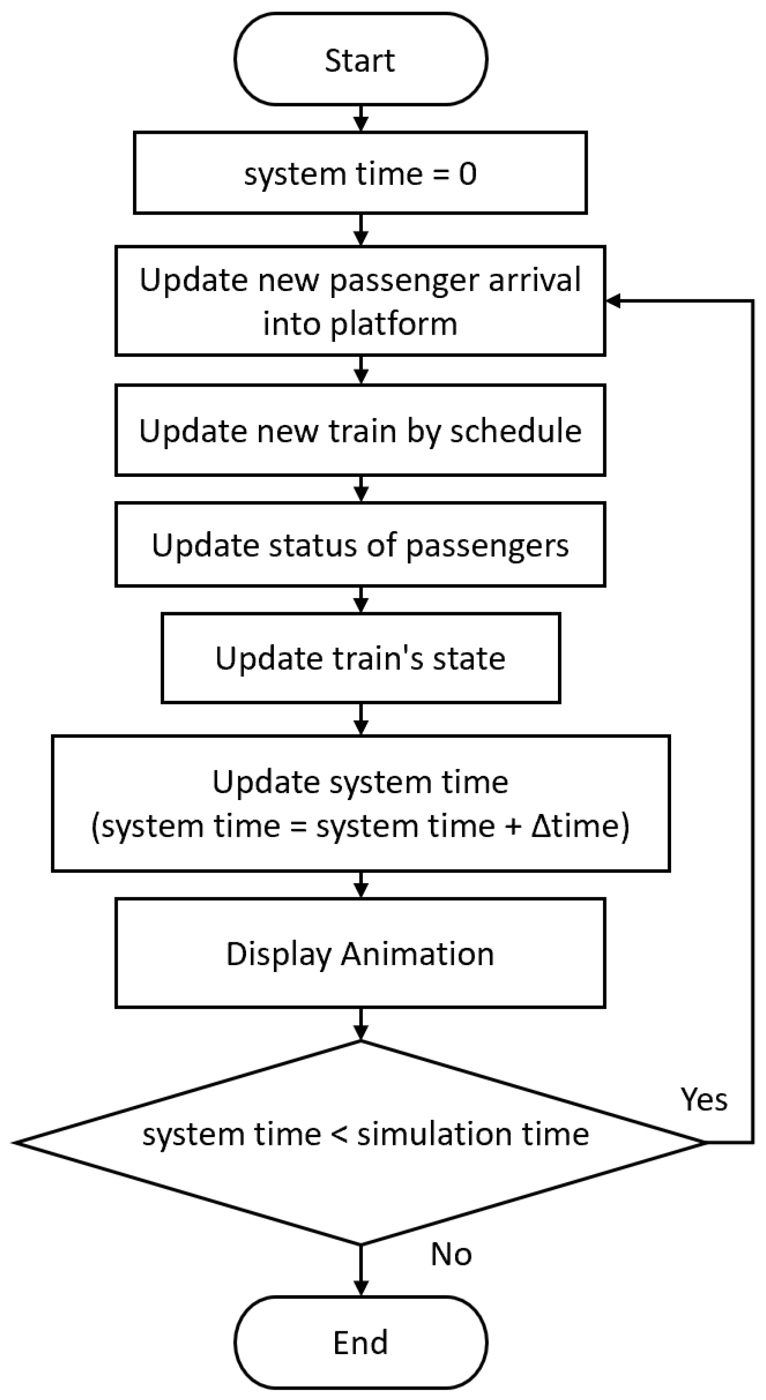
3.1. Developed Simulation

In the current study, by considering almost all main requirements and assumptions, we develop a comprehensive simulation model using the Python 3.9 environment according to the requirements defined by the Bangkok railway system. Our Python simulation uses the NumPy library to generate the number of passengers with random variables and the TKinter library to create the graphical user interface. There are four main processes in our Python simulation for the railway system.

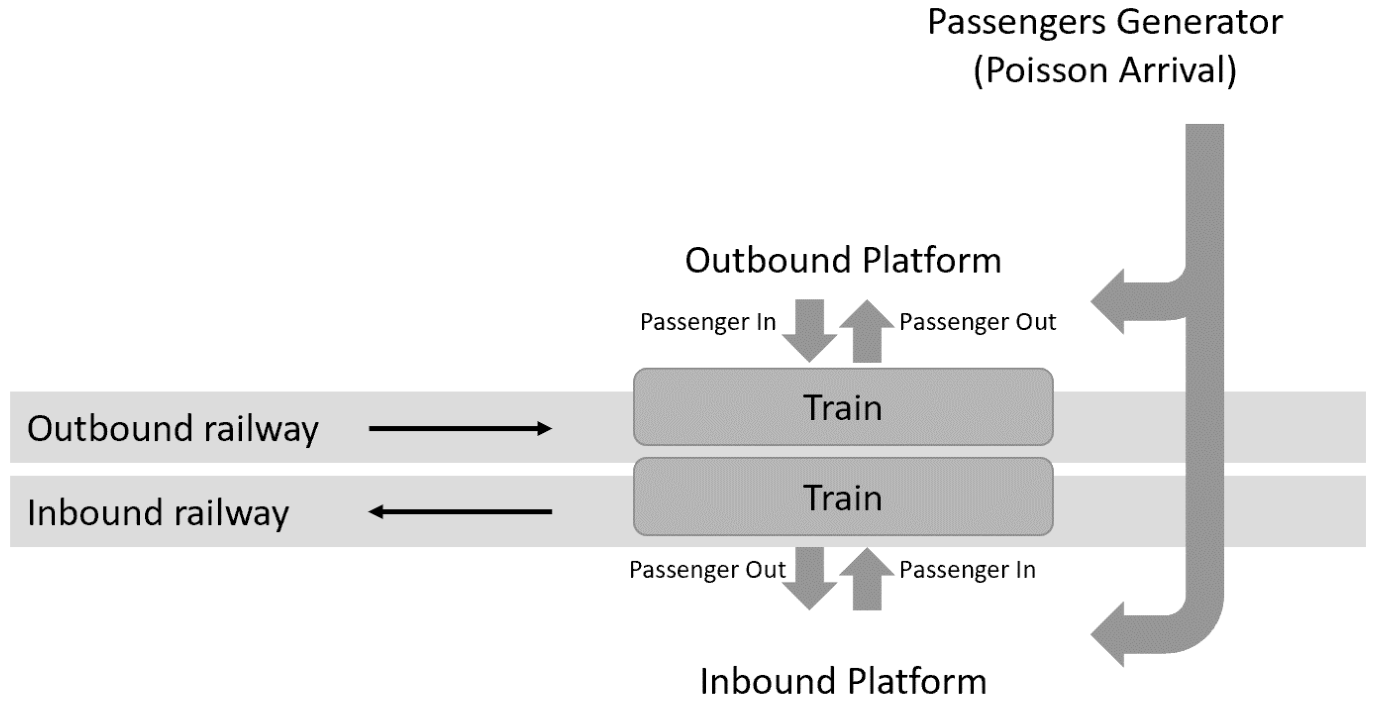
3.1.1. Passenger Arrival

Passengers were generated into the system with the origin station, arrival time, and destination. Given $a_{(s,p,h)}$, the number of arrival passengers at the station s in an hour-long period p and waiting for the train for headway $h_p$ was computed using random variables with a Poisson distribution, which is computed as follows:

$$Prob(a_{s,p,h}=k)=\frac{{\left({\lambda }_{s,p}{h}_p\right)}^k{e}^{-\left({\lambda }_{s,p}{h}_p\right)}}{k!}$$

(1)

where ${\lambda }_{s,p}$ is the expected values or passenger rate, which is calculated from our datasets that provides $A_{s,p}$, which is the number of arriving passengers at station s and in period p. To consider uncertainty in the rate of arrival of passengers, we assumed the three different scenarios and obtained an optimization result for each scenario separately. Note that the third scenario, called the worst-case scenario, is a common approach in robust optimization methodology (see [15,16,17]):

$$\begin{array}{cc}\hfill \mathrm{First}\mathrm{scenario}:& Avg\left(Arrival\right)+Std\left(Arrival\right)\hfill \\ \hfill \mathrm{Sec}\mathrm{ond}\mathrm{scenario}:& Avg\left(Arrival\right)+2\ast Std\left(Arrival\right)\hfill \\ \hfill \mathrm{Third}\mathrm{scenario}:& Avg\left(Arrival\right)+3\ast Std\left(Arrival\right)\hfill \end{array}$$

(2)

We assumed a Gaussian (normal) distribution for the uncertainty scenario (U) for both the arrival and departure rates. The first scenario covered 68.27% of the cases. The second and third (worst-case) scenarios covered 95.45% and 99.7% of the cases, respectively (see Figure 2). The generated passengers would wait for the train at the platform, which was separated into two types based on the train line direction: outbound or inbound. When the train arrived at the platform, the passengers would move to the train, and the waiting time for each passenger was collected (see Figure 3).

The total number of persons waiting at station s to take train n can be computed by

$$P{W}_{n,s}=a_{n,s,h}+P{R}_{n-1,s}$$

(3)

where $P{R}_{n-1,s}$ depicts the number of passengers that remain from the previous train ($n-1$) and are still waiting to take the current train (n) while the expression $a_{n,s,h}$ shows the number of passengers that just arrived at the station and are waiting to take a train. The number of passengers inside train n after boarding a train at station s is

$$P{T}_{n,s}=P{T}_{n,s-1}+P{W}_{n,s}-d_{n,s}-P{R}_{n,s}$$

(4)

where in the first station $(s=1)$, for all trains $n=1,2,\cdots ,N$, we assume $P{T}_{n,1}=0$. In Equation (4), the expression $P{T}_{n,s-1}$ shows the number of passengers on the train that already came from the previous station, and the expression $P{R}_{n,s}$ shows the number of passengers that could not take the current train (n) and had to wait until the next train ($n+1$) arrived. Meanwhile, $d_{n,s}$ reveals the number of passengers dropped off by train n at the current station (s). The expression $P{P}_{n,s}=P{T}_{n,s-1}+P{W}_{n,s}-d_{n,s}$ depicts the total number of possible passengers for train n. Therefore, the number of persons at station s that could not take train n because of the excess capacity of a train and had to wait for the next train is computed by

$$P{R}_{n,s}=\left\{\begin{array}{cc}P{P}_{n,s}-\mathrm{Capacity},\hfill & \mathrm{if}P{P}_{(n,s)}>\mathrm{Capacity}\hfill \\ 0,\hfill & \mathrm{otherwise}\hfill \end{array}\right.$$

(5)

3.1.2. Train Scheduler

The trains were generated in the system by a schedule that defined the time between trains (headway $h_p$) for each hour. The time $T{A}_{n,s}$ when train n arrived in station s is computed by

$$T{A}_{n,s}=T{A}_{n,s-1}+T{S}_{s-1}+T{T}_{(s-1)\to s}$$

(6)

where $T{S}_s$ is the time (in minutes) that the train stops at station s to pick up and drop off passengers, $T{T}_{s\to s+1}$ is the travel time (minutes) of a train between station s and the next station $s+1$ (assuming a fixed average speed), $n=1,2,\cdots ,N$, and $s=1,2,\cdots ,S$. Let us assume that $T{S}_0=0$, $T{T}_{0\to 1}=0$, and for the first station ($s=1$), we have

$$T{A}_{n,1}=(n-1)h_p+60(p-1)$$

(7)

The total number of trains N is computed by

$$N{T}_p=\frac{60}{h_p}+1,for(p=1,2,\cdots ,P)N=\sum _{p+1}^{P}N{T}_p$$

(8)

where $N{T}_p$ is the number of trains traveling in period $p=1,2,\cdots ,P$. The processes of the train contain three states: idle, moving, and braking (see Figure 4):

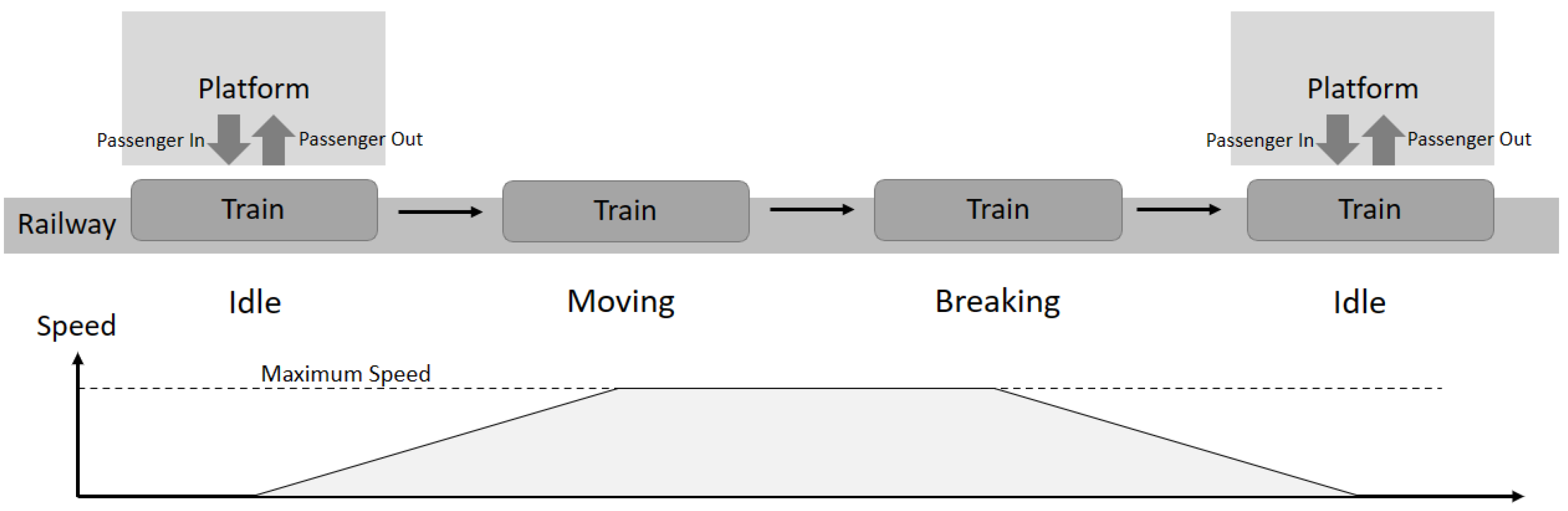
• In the idle state, the train stops at the station for dropping off and picking up passengers. If the number of passengers reaches the train’s capacity, then that train cannot pick up more passengers. After the stopping time, a train will collect the data on the number of passengers and enter the moving state.
• In the moving state, the speed of the train will accelerate until the maximum speed with constant train acceleration. Then, the train will retain this speed until reaching the braking distance and enter the braking state.
• In the braking state, the train will reduce its speed by deceleration, which is negative acceleration. The train will breke until its speed is zero at the next train station and reach the idle state again.

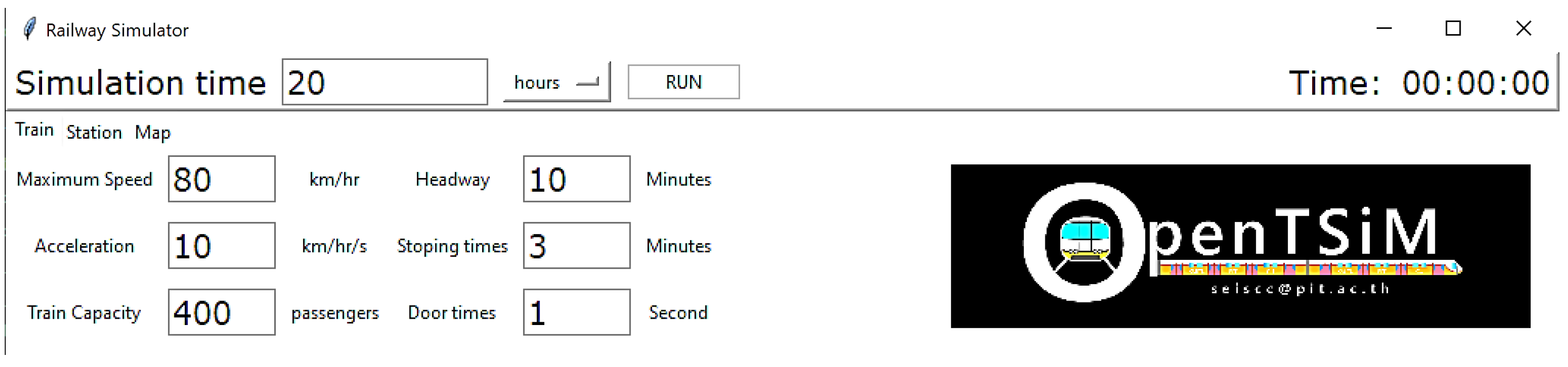
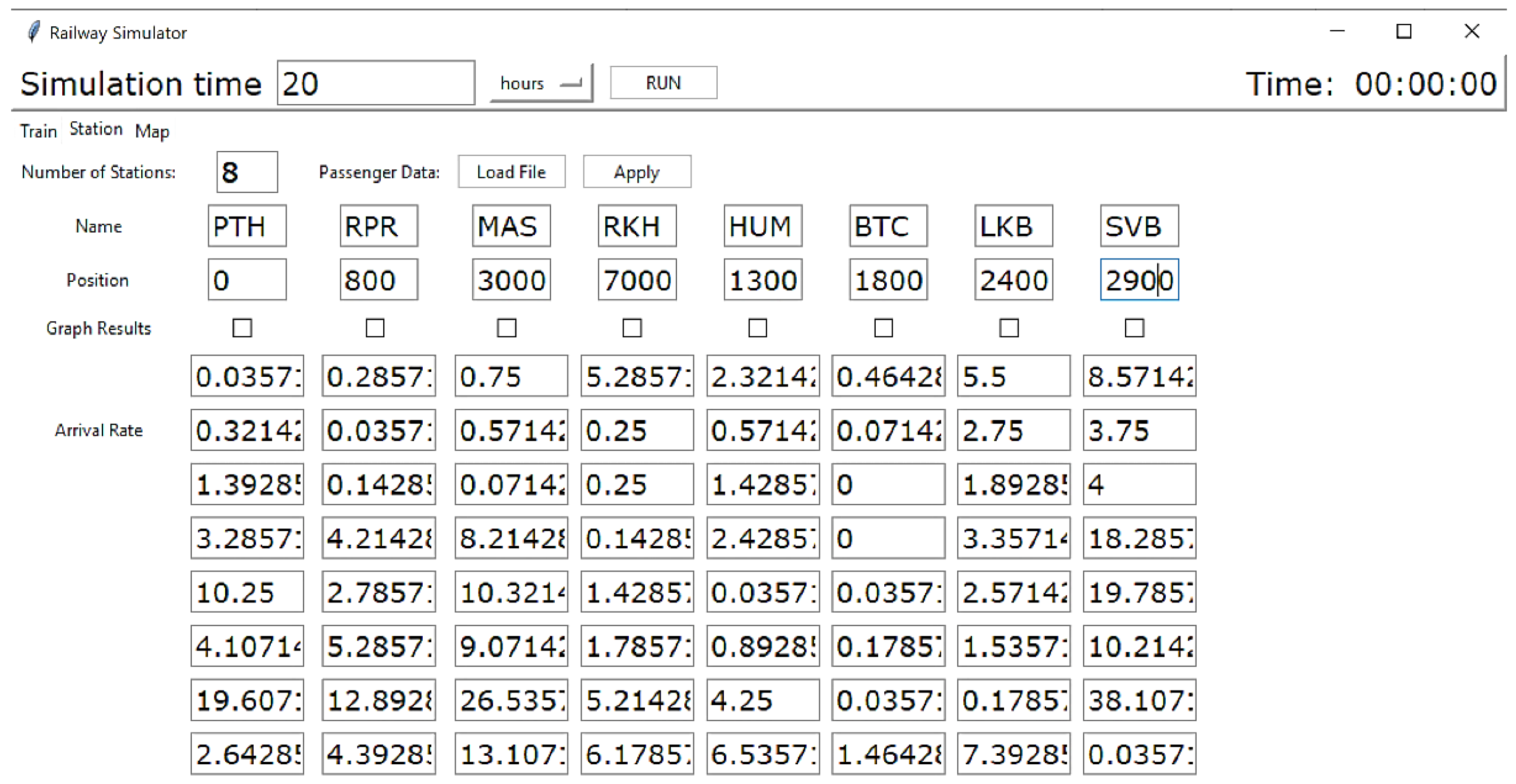
3.1.3. Parameter Declaration

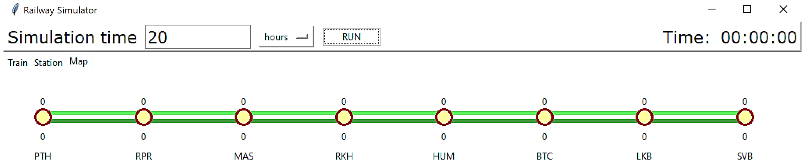
This process involves the graphical user interface (GUI) for parameter declaration. There are two types of parameters:

• Train parameters, including maximum speed, headway, acceleration, stopping time, train capacity, and door time (see Figure 5);
• Station parameters, including station name, the position of the station, and passengers’ arrival rate (see Figure 6).

3.1.4.  Animation

This subsection presents how the railway system is simulated in the GUI, shown in Figure 7.

The Python simulation started with a system time of zero. The passenger’s arrival would be updated when the system time equaled the arrival time of the passenger. The trains would be generated in the system by the train scheduler. Next, the system would update all passengers’ and trains’ states and then display the system in the animation. This loop would be continued until the end of the simulation time. Figure 8 shows the illustrated flow diagram of our simulation procedure.

3.2. Searching Optimal Headways

Following our developed simulation model, to run simulation experiments and investigate the optimal headway for each time interval using a real dataset from the Bangkok railway system, we integrated the common PSO algorithm with our simulation prototype. The canonical PSO algorithm that simulates the swarm behaviors of social animals, such as bird flocking or fish schooling, was proposed in [18]. The parameters of PSO consist of the number of particles, position of the agent in the solution space, velocity, and neighborhood of agents (communication of topology). The PSO algorithm begins by initializing the population. The second step is calculating the fitness values of each particle, followed by updating the individual and global bests, and later, the velocity and the position of the particles are updated. The second through fourth steps are repeated until the termination condition is satisfied. The PSO algorithm is formulated as follows [18]:

$$\begin{array}{c}\hfill v_{id}^{t+1}=v_{id}^t+c_{1}rand(0,1)(p_{id}^t-x_{id}^t)+c_{2}rand(0,1)(p_{id}^t-x_{id}^t)\end{array}$$

(9)

$$x_{id}^{t+1}=x_{id}^t+v_{id}^t$$

(10)

where $v_{id}^t$ and $x_{id}^t$ are the particle velocity and particle position, respectively, d is the dimension in the search space, i is the particle index, and t is the iteration number. Expressions $c_1$ and $c_2$ represent the speed, regulating the length when flying toward the most optimal particles of the whole swarm and the most optimal individual particle. The term $p_i$ is the best position achieved thus far by particle i, and $p_g$ is the best position found by the neighbors of particle i. The expression rand (0, 1) shows the random values between 0 and 1. The exploration happens if either or both of the differences between the particle’s best ($p_{id}^t$) and the previous particle’s position ($x_{id}^t$) and between the population’s all-time best ($p_{id}^t$) and the previous particle’s position ($x_{id}^t$) are large, and exploitation occurs when these values are both small. PSO has attracted wide attention in timetable scheduling and railway optimization problems due to its algorithmic simplicity and powerful search performance (see [19,20,21,22]).

4. Experiments and Results

4.1. Simulation Set-Up and Parameter Adjustment

In this context, two objective functions include minimizing the average wait time of passengers and minimizing the average number of operating trains [23,24]. The first objective function is defined to take into account customer satisfaction, and the second objective function considers the railway operating cost (operating trains) [25,26]. For this purpose, we considered the two separate objective functions shown below:

$$f_1:\mathrm{average}\mathrm{waiting}\mathrm{time}\mathrm{over}\mathrm{all}\mathrm{stations}\mathrm{in}\mathrm{each}\mathrm{time}\mathrm{interval}$$

(11)

$$f_2:\mathrm{number}\mathrm{of}\mathrm{trains}\mathrm{operating}\mathrm{in}\mathrm{each}\mathrm{time}\mathrm{interval}$$

(12)

To combine both objective functions into an overall objective, we used the weighted function below:

$$MinimizeF=\omega {\tilde{f}}_1+(1-\omega ){\tilde{f}}_2$$

(13)

where $\omega$ is a weight factor $(0\le \omega \le 1)$ and ${\tilde{f}}_1$ and ${\tilde{f}}_2$ are the first objective and the second objective functions that are normalized in [0, 1] to be on the same scale, respectively [27,28]. According to Equation (13), the optimal result depends on the values of $\omega$, which can be chosen by the decision maker. Varying this magnitude provides the capture of the Pareto frontier (also called the Pareto optimal efficiency) to make a trade-off between different objectives. This approach is a classical method to solving optimization problems when the model is faced with multiple criteria [29,30]. The set of optimal solutions obtained from fluctuating $\omega$ in the range [0, 1] provides an estimate of the Pareto frontier. In the current optimization model, the design variables are assumed to be a headway (gap of time between travel for every two sequential trains) in each time interval [31,32]. (Here, 19 time intervals were assumed regarding the working hours in a day.) The lower and upper range for the headways were assumed to be [5, 15] min. Additionally, we assumed that the difference in headways between the two following time intervals had to be less than 5 min. Three uncertainty scenarios were considered for the arrival rate regarding the Gaussian probability (see Section 3.1). The case study considered in this paper is an urban transit network located within the metropolitan area of Bangkok, the capital city of Thailand. The network currently includes eight stations (PTH, RPR, MAS, RKH, HUM, BTC, LKB, and SVB) in two directions. More details on the Bangkok railway system were mentioned in Section 2. The real data, including arrival and departure rates, were collected for one month (from 1 to 28 February 2021) from the control office of the railway. The collected data were gathered separately for weekdays and weekends. In the current study, in order to evaluate our developed simulation model, we averaged all the data collected for one month based on the arrival and departure rates for each direction, each station, and each time interval (i.e., working hours per day) separately for use as sample data in the simulator. To investigate the optimal headways using the PSO optimizer, the initial population was adjusted to 40, and the number of iterations was considered to be 30. The other parameters for PSO were also adjusted as follows: min of inertia weight = 0.4, max of inertia weight = 0.9, and all the three factors of the velocity clamping factor, cognitive constant, and social constant being set to 2. The developed Python-based simulation was run, and the relevant results were obtained. The overall collected results are provided and discussed in the next subsection.

4.2. Result Optimization

In this section, we present the dataset and results obtained from the simulation experiments and optimization algorithms. The developed Python-based simulator was set up by considering assumptions and model parameters which were adjusted according to the previous section. Here, the weight scale $\omega$ in Equation (13) was considered to be 0.5, which means both objective functions including an average wait time and a number of required operating trains were assumed to be of the same importance in an optimization procedure. In the railway system under study, two straight and return pathways from and to Suvarnabhumi airport were considered. Figure 9 and Figure 10 illustrate the collected arrival and departure rates (number of passengers) at each station and for each pathway. As mentioned before, we first employed the average arrival and departure rates from the real data collected from the Bangkok railway system over one month and used these rates in our simulator. The PSO optimizer was derived by connecting with the developed Python-based simulation model to run simulation experiments and investigate the optimal headway results.

Table 3. The optimal headways and objective functions (wait time and number of operating trains) for $\omega =0.5$.

Time Intervals	Optimal Headway	Waiting Time			Operating Trains
		Minutes	Avg.	Std.	Number	Avg.	Std.
5–6 am	6.79	12.63	11.02	1.65	5.00	6.54	0.50
6–7	10.11	7.86			5.91
7–8	6.94	7.60			6.08
8–9	6.21	9.11			6.75
9–10	6.63	10.71			7.20
10–11	10.12	10.25			7.17
11–12	6.30	9.95			7.08
12–13	8.87	9.72			7.12
13–14	10.98	10.01			6.95
14–15	11.15	10.43			6.77
15–16	13.34	11.21			6.63
16–17	12.05	11.90			6.50
17–18	7.68	12.01			6.45
18–19	8.62	12.15			6.45
19–20	7.11	12.47			6.47
20–21	8.26	12.46			6.51
21–22	10.70	12.70			6.47
22–23	13.93	12.97			6.42
23–24	10.95	13.21			6.38

provides the obtained optimal headways and the relevant two objective functions accordingly. As can be seen from the table, the simulation provided reliable results according to the total average wait time for all eight stations and also the number of required trains in each time interval. In such a time interval faced with a higher average number of passengers for all stations, the smaller headway (travel time between every two following trains) computed provided small variability for the average wait time and the number of operating trains. In other words, the maximum of 13.21 min and minimum of 7.60 min with a standard deviation of 1.65 min for the average wait time for all time intervals, including crowd peak times, were obtained. The same pattern can be seen for the number of required trains that operated at each time interval per day.

5. Discussion

In this section, the sensitivity of the obtained results from the simulation-based optimization model is analyzed regarding two aspects: the weight scale $\omega$ in Equation (13) and according to the uncertainty in the arrival rate, referring to Equation (2). To analyze the optimization model regarding $\omega$, we ran the simulation model and used the optimization algorithm for different values of $\omega$, obtaining the Pareto frontier results. Figure 11 depicts the optimal headways for different values of $\omega$ in Equation (13), and Figure 12 shows the results of Pareto frontier estimation obtained by varying the weight scale parameter $\omega$. As can be seen from the results, when $\omega$ was close to one, this meant that the importance of the first objective (average wait time) was greater than the second objective (number of operating trains), and smaller headways were obtained for each time interval. Conversely, when $\omega$ was close to zero, and the number of operating trains (railway system cost) was more important, the headways became larger for all time intervals. Additionally, the same trend is clear in the results shown in Figure 12. Aside from analyzing the model regarding $\omega$, we also analyzed the optimization results for the uncertainty in the arrival rate of passengers. For this purpose, as described in subsection A, three different scenarios were considered for the arrival rate, integrating the average and standard deviation of the arrival rate obtained from collected data over all 28 days (February 2021) under study. We ran the simulation model using the optimal headways that are already obtained considering and computing the waiting time for different scenarios. Note that as we used the same headways for all three scenarios, the number of operating trains did not change compared to the original model. As shown in

Table 4. Effect of uncertainty over first objective function (average wait time) for three different uncertainty scenarios due to variability in arrival rates on different days of month under study.

Weight Factor	Average over Arrival Rates ( for All Days)		Scenario 1 (Avg. + Std.)		Scenario 2 (Avg. + 2 Std.)		Scenario 3 (Avg. + 3 Std.)
	Avg.	Std.	Avg.	Std.	Avg.	Std.	Avg.	Std.
1	4.55	1.62	18.56	6.48	10.58	3.05	5.09	0.48
0.9	6.94	1.68	41.52	23.52	30.08	15.50	16.19	6.40
0.8	8.82	1.58	51.44	33.82	37.53	17.21	18.20	5.00
0.7	8.87	2.06	54.98	42.23	41.19	24.16	20.85	6.65
0.6	12.59	1.78	53.56	27.92	41.81	17.92	25.85	7.96
0.5	11.02	1.65	51.74	33.79	43.12	22.83	26.46	10.95
0.4	20.81	5.37	63.75	41.95	58.34	38.03	45.46	23.27
0.3	30.27	10.92	66.82	42.94	61.34	40.91	53.95	30.01
0.2	43.04	22.36	87.51	61.42	74.55	50.74	58.76	36.24
0.1	58.34	31.43	124.20	70.43	100.82	58.73	81.08	47.96
0	55.76	33.33	117.07	70.81	93.90	61.78	75.90	46.38

, by adding the average arrival rate with a fixed coefficient for the standard deviation and increasing the number of passengers who arrived at the stations, there was a greater average wait time (as expected) in the practical railway environment. This also confirms the effectiveness of our developed simulation model in optimizing and analyzing the sensitivity of the Bangkok railway system in a real-world environment.

6. Conclusions and Future Work

In this work, we optimized the railway resource allocations (i.e., the required number of operating trains) for a railway line which connects Suvarnabhumi Airport to the center of Bangkok, called the airport rail link, while minimizing the passenger wait time to enhance customer satisfaction. To achieve this, a multi-objective PSO method was derived to compute the Pareto front with different optimal train headways, thereby identifying the best real-time train timetables. As the past actual traffic data used to construct the simulation-based optimization model were very comprehensive, where the arrival time of each individual passenger was collected and exploited, the numerical results from our proposed model can be readily deployed in practice. In addition, the optimum number of operating trains was obtained for each hour in the day. Moreover, the proposed model can provide an exchange between the number of operating trains and the passenger wait times, which can be an effective service tool for railway operators. The results obtained using a real dataset from the Bangkok railway system demonstrate that the simulation-based optimization approach for robust train service timetable scheduling, which incorporates both passenger wait times and the number of operating trains as equally important objectives, successfully achieved an average waiting time of 11.02 min (with a standard deviation of 1.65 min) across all time intervals. Due to the data and focus problem in the ARL, these results represented that we can apply the PSO optimization technique with our simulation tool to observing the headway in normal or uncertain situations. Anyway, this technique and our open-source tool can be applied to other lines in Bangkok by modifying the structure of the train within the condition of a single train line for now. Our tools with the PSO optimizer can be improved for the other railway’s system in the near future.

References

1. Yang, X.; Li, X.; Gao, Z.; Wang, H.; Tang, T. A cooperative scheduling model for timetable optimization in subway systems. IEEE Trans. Intell. Transp. Syst. 2012, 14, 438–447. [Google Scholar] [CrossRef]
2. Silva, J.C.; Saadi, M.; Wuttisittikulkij, L.; Militani, D.R.; Rosa, R.L.; Rodríguez, D.Z.; Al Otaibi, S. Light-field imaging reconstruction using deep learning enabling intelligent autonomous transportation system. IEEE Trans. Intell. Transp. Syst. 2021, 23, 1587–1595. [Google Scholar] [CrossRef]
3. Hansen, I.A. Railway Timetable & Traffic: Analysis, Modelling, Simulation; Eurailpress: Hamburg, Germany, 2008. [Google Scholar]
4. Saadi, M.; Noor, M.T.; Imran, A.; Toor, W.T.; Mumtaz, S.; Wuttisittikulkij, L. IoT enabled quality of experience measurement for next generation networks in smart cities. Sustain. Cities Soc. 2020, 60, 102266. [Google Scholar] [CrossRef]
5. Available online: https://datagov.mot.go.th/dataset/stat_pass_rail/resource/b72f1a21-72f3-47f2-851b-6d92a93351d4 (accessed on 21 November 2022).
6. Cacchiani, V.; Toth, P. Nominal and robust train timetabling problems. Eur. J. Oper. Res. 2012, 219, 727–737. [Google Scholar] [CrossRef]
7. Khan, M.A.; Ghosh, S.; Busari, S.A.; Huq, K.M.S.; Dagiuklas, T.; Mumtaz, S.; Iqbal, M.; Rodriguez, J. Robust, resilient and reliable architecture for v2x communications. IEEE Trans. Intell. Transp. Syst. 2021, 22, 4414–4430. [Google Scholar] [CrossRef]
8. Ribeiro, D.A.; Silva, J.C.; Lopes Rosa, R.; Saadi, M.; Mumtaz, S.; Wuttisittikulkij, L.; Zegarra Rodriguez, D.; Al Otaibi, S. Light field image quality enhancement by a lightweight deformable deep learning framework for intelligent transportation systems. Electronics 2021, 10, 1136. [Google Scholar] [CrossRef]
9. Caimi, G.; Kroon, L.; Liebchen, C. Models for railway timetable optimization: Applicability and applications in practice. J. Rail Transp. Plan. Manag. 2017, 6, 285–312. [Google Scholar] [CrossRef]
10. Li, W.; Zhang, T.; Wang, R.; Huang, S.; Liang, J. Multimodal multi-objective optimization: Comparative study of the state-of-the-art. Swarm Evol. Comput. 2023, 77, 101253. [Google Scholar] [CrossRef]
11. Ribeiro, A.D.; Melgarejo, D.; Saadi, M.; Rosa, L.; Rodríguez, D. A novel deep deterministic policy gradient model applied to intelligent transportation system security problems in 5G and 6G network scenarios. Phys. Commun. 2023, 56, 101938. [Google Scholar] [CrossRef]
12. Song, T.; Tang, T.; Xun, J.; Wang, H.; Gao, S. Train headway adjustment using potential function based on multi-agent formation control. In Proceedings of the 2018 International Conference on Intelligent Rail Transportation (ICIRT), Singapore, 12–14 December 2018; pp. 1–5. [Google Scholar]
13. Zhao, Y.; Ioannou, P. Positive train control with dynamic headway based on an active communication system. IEEE Trans. Intell. Transp. Syst. 2015, 16, 3095–3103. [Google Scholar] [CrossRef]
14. Weerawat, W.; Samitiwantikul, R.; Torpanya, L. Operational Challenges of the Bangkok Airport Rail Link. Urban Rail Transit 2020, 6, 42–55. [Google Scholar] [CrossRef]
15. Parnianifard, A.; Azfanizam, A.S.; Ariffin, K.M.; Ismail, M.I.S. Kriging-Assisted Robust Black-Box Simulation Optimization in Direct Speed Control of DC Motor Under Uncertainty. IEEE Trans. Magn. 2018, 54, 1–10. [Google Scholar] [CrossRef]
16. Goli, A.; Zare, K.H.; Moghaddam, T.; Sadeghieh, A.R. Hybrid artificial intelligence and robust optimization for a multi-objective product portfolio problem Case study: The dairy products industry. Comput. Ind. Eng. 2019, 137, 106090. [Google Scholar] [CrossRef]
17. Beyer, H.G.; Sendhoff, B. Robust optimization—A comprehensive survey. Comput. Methods Appl. Mech. Eng. 2007, 196, 3190–3218. [Google Scholar] [CrossRef]
18. Shami, T.M.; El-Saleh, A.A.; Alswaitti, M.; Al-Tashi, Q.; Summakieh, M.A.; Mirjalili, S. Particle Swarm Optimization: A Comprehensive Survey. IEEE Access 2022, 10, 10031–10061. [Google Scholar] [CrossRef]
19. Kim, K.; Kim, J.; Lee, C.; Kim, J.; Lee, H. PSO-Based Initial SOC and Capacity Optimization for Stationary Energy Storage Systems in DC Electric Railway System. J. Electr. Eng. Technol. 2021, 16, 2281–2289. [Google Scholar] [CrossRef]
20. Pan, Z.; Chen, M.; Lu, S.; Tian, Z.; Liu, Y. Integrated timetable optimization for minimum total energy consumption of an AC railway system. IEEE Trans. Veh. Technol. 2020, 69, 3641–3653. [Google Scholar] [CrossRef]
21. Li, J.; Wei, W.; He, Y. Optimization of online timetable re-scheduling in high-speed train services based on PSO. In Proceedings of the 2011 International Conference on Transportation, Mechanical, and Electrical Engineering (TMEE 2011), Changchun, China, 16–18 December 2011; pp. 1896–1899. [Google Scholar] [CrossRef]
22. Ho, K.T.; Tsang, C.W.; Ip, K.H.; Kwan, K.S. Train service timetabling in railway open markets by particle swarm optimisation. Expert Syst. Appl. 2012, 39, 861–868. [Google Scholar] [CrossRef]
23. Parnianifard, A.; Chancharoen, R.; Phanomchoeng, G.; Wuttisittikulkij, L. A New Approach for Low-Dimensional Constrained Engineering Design Optimization Using Design and Analysis of Simulation Experiments. Int. J. Comput. Intell. Syst. 2020, 13, 1663–1678. [Google Scholar] [CrossRef]
24. Zhou, Z.; Liu, P.; Feng, J.; Zhang, Y.; Mumtaz, S.; Rodriguez, J. Computation resource allocation and task assignment optimization in vehicular fog computing: A contract-matching approach. IEEE Trans. Veh. Technol. 2019, 68, 3113–3125. [Google Scholar] [CrossRef]
25. Li, W.; Peng, Q.; Wen, C.; Xu, X. Comprehensive optimization of a metro timetable considering passenger waiting time and energy efficiency. IEEE Access 2019, 7, 160144–160167. [Google Scholar] [CrossRef]
26. Zhao, N.; Roberts, C.; Hillmansen, S.; Nicholson, G. A multiple train trajectory optimization to minimize energy consumption and delay. IEEE Trans. Intell. Transp. Syst. 2015, 16, 2363–2372. [Google Scholar] [CrossRef]
27. Sun, X.; Zhang, S.; Dong, H.; Zhu, H. Optimal train schedule with headway and passenger flow dynamic models. In Proceedings of the 2013 IEEE International Conference on Intelligent Rail Transportation (ICIRT 2013), Beijing, China, 30 August–1 September 2013; pp. 307–312. [Google Scholar] [CrossRef]
28. Yalçınkaya, Ö.; Bayhan, G.M. Modelling and optimization of average travel time for a metro line by simulation and response surface methodology. Eur. J. Oper. Res. 2009, 196, 225–233. [Google Scholar] [CrossRef]
29. Xu, L.; Zhao, X.; Tao, Y.; Zhang, Q.; Liu, X. Optimization of train headway in moving block based on a particle swarm optimization algorithm. In Proceedings of the 2014 13th International Conference on Control, Automation, Robotics & Vision (ICARCV 2014), Singapore, 10–12 December 2014; pp. 931–935. [Google Scholar] [CrossRef]
30. Cacchiani, V.; Furini, F.P.; Kidd, M. Approaches to a real-world train timetabling problem in a railway node. Omega 2016, 58, 97–110. [Google Scholar] [CrossRef]
31. Yang, X.; Chen, A.; Ning, B.; Tang, T. A stochastic model for the integrated optimization on metro timetable and speed profile with uncertain train mass. Transp. Res. Part B Methodol. 2016, 91, 424–445. [Google Scholar] [CrossRef]
32. Shang, P.; Li, R.; Yang, L. Optimization of urban single-line metro timetable for total passenger travel time under dynamic passenger demand. Procedia Eng. 2016, 137, 151–160. [Google Scholar] [CrossRef]
Figure 1. Structure of airport rail link (ARL).
Electronics 12 03493 g001
Figure 2. Different intervals and relevant probability for arrival and departure rates in model with Gaussian probability distribution.
Electronics 12 03493 g002
Figure 3. Model of passenger generator and platforms.
Electronics 12 03493 g003
Figure 4. Arrival and departure rates of the train following the Gaussian probability distribution.
Electronics 12 03493 g004
Figure 5. States of trains.
Electronics 12 03493 g005
Figure 6. Graphical user interface of train parameter configuration.
Electronics 12 03493 g006
Figure 7. Graphical user interface of station parameter configuration.
Electronics 12 03493 g007
Figure 8. Flow diagram of passenger and train simulation in railway system using Python.
Electronics 12 03493 g008
Figure 9. Schematic showing number of passengers that arrived at each station and each pathway.
Electronics 12 03493 g009
Figure 10. Schematic showing number of passengers that departed from each station with regard to each pathway.
Electronics 12 03493 g010
Figure 11. Optimal headways regarding different values of ω in Equation (13).
Electronics 12 03493 g011
Figure 12. Varying the parameter ω in Equation (13) and Pareto frontier results for each of two conflicting objective functions.
Electronics 12 03493 g012