Research on Non-Intrusive Load Recognition Method Based on Improved Equilibrium Optimizer and SVM Model

Abstract

Non-intrusive load monitoring is the main trend of green energy-saving electricity consumption at present, and load identification is a core part of non-invasive load monitoring. A support vector machine (SVM) is commonly used in load recognition, but there are still some problems in the parameter selection, resulting in a low recognition accuracy. Therefore, an improved equilibrium optimizer (IEO) is proposed to optimize the parameters of the SVM. Firstly, household appliance data are collected, and load features are extracted to build a self-test dataset; and secondly, Bernoulli chaotic mapping, adaptive factors and the Levy flight were introduced to improve the traditional equilibrium optimizer algorithm. The performance of the IEO algorithm is validated on test functions, and the SVM is optimized using the IEO algorithm to establish the IEO-SVM load identification model. Finally, the recognition effect of the IEO-SVM model is verified based on the self-test dataset and the public dataset. The results show that the IEO algorithm has good optimization accuracy and convergence speed on the test function. The IEO-SVM load recognition model achieves an accuracy of 99.428% on the self-test dataset and 100% accuracy on the public dataset, and the classification performance is significantly better than other classification algorithms, which can complete the load recognition task well.

1. Introduction

Along with the intensification of global energy consumption, energy savings and emission reduction, green environmental protection has become the mainstream of the current energy revolution. Under the strong impetus of the Internet of Things, the smart grid has become one of the representatives of the energy revolution. Smart electricity consumption is an important part of the smart grid, which is in line with the strategic goal of “carbon neutrality” to reduce the resource waste of electricity [1]. Non-intrusive load monitoring (NILM) technology is a key technology for intelligent electricity consumption. By monitoring customers’ electrical energy data, accurate load information can be obtained, such as the type of load. This load information can improve the efficiency of power utilization on the grid side and assist in adjusting power consumption strategies on the customer side [2,3,4].

Non-intrusive load monitoring is divided into four steps: data acquisition, event monitoring, feature extraction and load identification, among which load identification is the most important [5]. In recent years, there has been significant research conducted by numerous scholars in the field of load identification, and the common recognition algorithms include k-nearest neighbor (k-NN) [6], artificial neural network (ANN) [7,8], support vector machines (SVM) [9], logistic regression (LR) [10], decision tree (DT) [11], etc. Ref. [12] used the energy of wavelet coefficients as load features and used decision trees for load identification, which effectively improved the classification accuracy. Ref. [13] proposed a V–I trajectory-based NILM method that utilizes trajectory preprocessing and color encoding for data processing, employs the AlexNet convolutional neural network for load classification, and validates the effectiveness of this method on the NILM dataset. Ref. [14] used a particle swarm algorithm to optimize ANN and established a PSO-ANN load recognition model to identify aging loads, and the recognition accuracy was improved. Ref. [15] fused multiple features such as V-I trajectories and harmonic amplitudes into a feature matrix and used a neural network for load identification, which is better for multi-state loads. Ref. [16] used the k-NN classification algorithm to classify and identify seven different household appliances in the REDD dataset, with better results for high-power appliances such as microwave ovens and washing machines. Ref. [17] used a low sampling rate smart meter to collect AC appliance data and built an SVM classification model, and the model can effectively identify the state of AC appliances. Ref. [18] used SVM for load identification of household appliance signals with a sampling frequency of 1 Hz to achieve the accurate identification of electric heating loads such as water heaters, but performed poorly in the identification of low-power appliances. Ref. [19] used a load identification method combining SVM and D–S evidence theory, and the recognition accuracy reached 85.5%, and the recognition could be improved. Ref. [20] used a particle swarm optimization (PSO) to optimize SVM and used the PSO-SVM model to identify electrical equipment, and the method exhibited better recognition accuracy. A multi-agent reinforcement learning framework for addressing the feature selection problem is proposed in Reference [21]. A stepwise hidden Markov model is used by [22] to decompose the active power time series. Ref. [23] utilizes an improved hidden Markov model for decomposition, achieving good stability but exhibiting poor classification accuracy. Ref. [24] employs a three-layer convolutional neural network for the classification and recognition of individual loads or combined loads, achieving good results on both self-test datasets and publicly available datasets. Ref. [25] introduces a load identification method based on active deep learning, which utilizes discrete wavelet transform to extract load features and establishes a three-layer convolutional neural network for classifying appliance samples. Ref. [26] combines multilayer perceptron, convolutional neural network, and long short-term memory to construct a deep learning model, and verifies the accuracy of this method on a real-world dataset. Ref. [27] introduces a binary mapping of voltage and current trajectories to classify seven types of front-end circuit topologies. Ref. [28] presents a deep learning network based on the CNN-LSTM framework, which performs sampling preprocessing on the real-world dataset and feeds it into CNN-LSTM for training and validation, accomplishing the task of load identification. Ref. [29] proposes a Bayesian optimization-based bidirectional long short-term memory method for non-intrusive load monitoring, which demonstrates superiority in performance. The above studies using k-NN, ANN, DT, LR and deep learning algorithms for load recognition may be affected by overfitting, model complexity and random initial weights, resulting in poor recognition results. In contrast, SVM adopts the principle of structural risk minimization and can solve the dimensional disaster problem by introducing kernel functions with strong fitting and generalization abilities, which makes SVM more suitable for solving practical classification problems. Although SVM has strong robustness, its recognition effect is limited when the SVM parameters are fixed. The traditional SVM parameters are selected based on manual experience and repeated trial and error, which result in difficulties ensuring that the optimal parameters are obtained.

To address the above problems, this paper proposes a load identification algorithm based on the improved equilibrium optimizer (IEO) algorithm to optimize the SVM. Subsequently, the optimized IEO-SVM method is employed for the identification and classification of household appliances, aiming to improve recognition accuracy. In the proposed method, three improvement strategies, namely Bernoulli chaotic mapping, adaptive factor and Levy flight, are employed to enhance the optimization capability of the EO algorithm. By utilizing the IEO algorithm to optimize the SVM, we can construct an optimal SVM model, namely the IEO-SVM model. To validate the classification performance of the IEO-SVM model, it is trained using datasets collected under laboratory conditions and public datasets. The trained model is then used to perform load recognition tasks and compared with existing methods. Experiments prove that the IEO-SVM model can better complete the load identification tasks and show good classification performance.

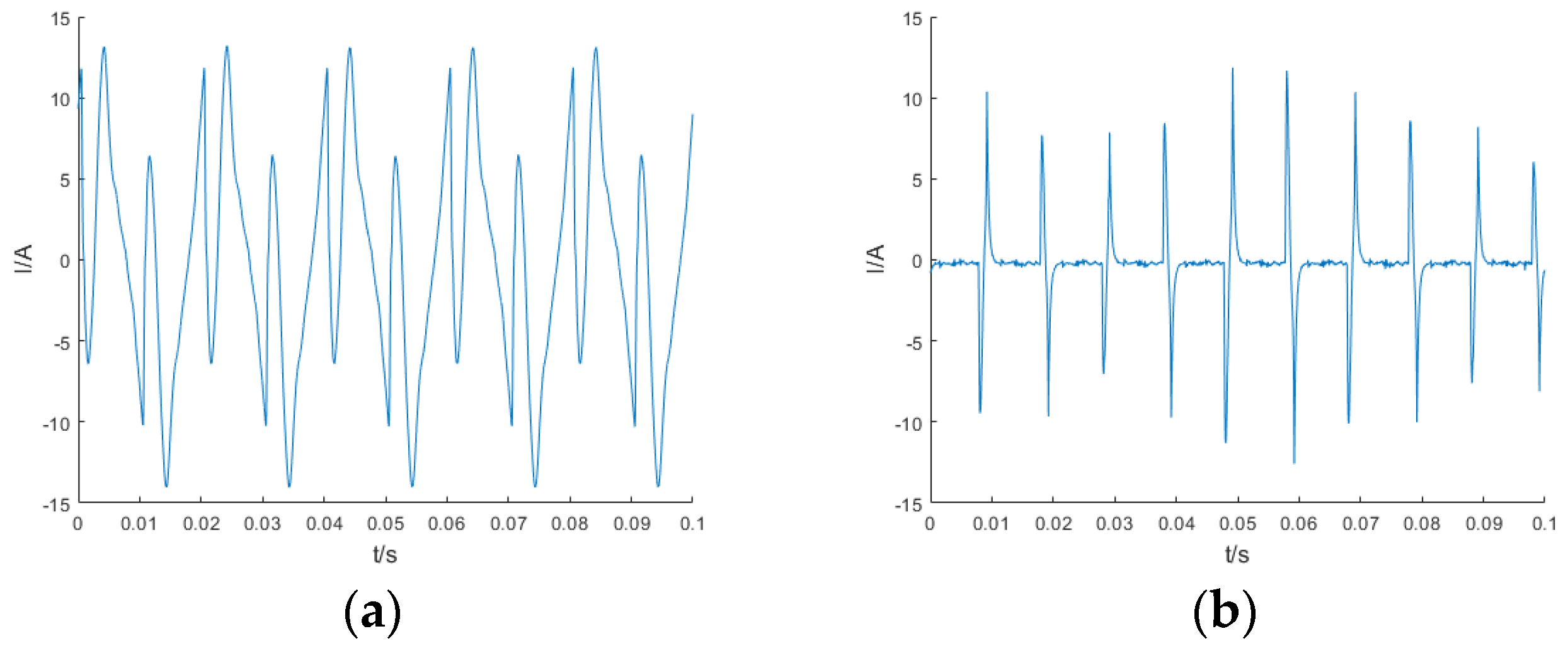
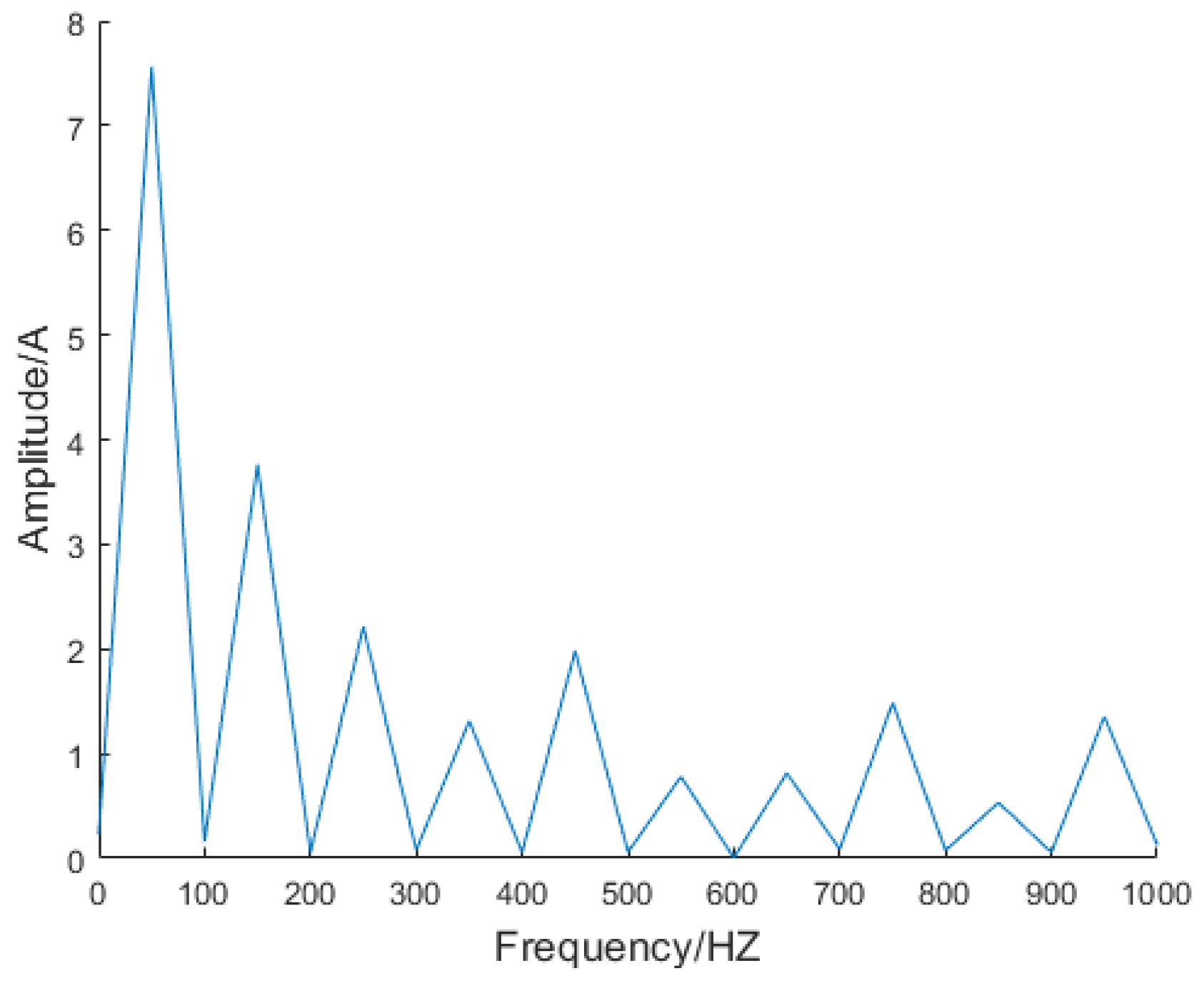
2. Home Load Feature Extraction and Data Pre-Processing

When studying certain signals, the recognition is not effective if the information is extracted directly from the original data. Therefore, extracting load features that can characterize the signal waveform is essential. The load steady-state feature refers to the feature quantity that can be extracted after the household appliances work stably. Load features are an important basis for completing load identification. Different load features have different abilities to distinguish loads. The current waveforms of the microwave oven (running state) and the laptop are shown in Figure 1. The load features selected in this paper are current peak $I_{peak}$, absolute value of current average $I_{avg}$, current variance $I_{\mathrm{var}}$, current root mean square value $I_{rms}$, and current harmonic amplitude $Hmc$. $I_{peak}$ is the maximum current value in one cycle; $I_{avg}$ is the degree of asymmetry of the positive and negative half-periods of the current waveform in one cycle; $I_{\mathrm{var}}$ is the trend of the current waveform; and $I_{rms}$ is the effective value of the current. As can be seen from Figure 1, $I_{peak}$, $I_{avg}$, $I_{\mathrm{var}}$ and $I_{rms}$ are different when different appliances are in stable operation and can therefore be used to identify the load features of electrical appliances.

The formulas of $I_{peak}$, $I_{avg}$, $I_{\mathrm{var}}$ and $I_{rms}$ are as follows.

$$I_{peak}=\max (I_1,I_2,\cdots ,I_N)$$

(1)

$$I_{avg}=\left|\frac{1}{N}{\displaystyle \sum _{i=0}^{N-1}{I}_i}\right|$$

(2)

$$I_{\mathrm{var}}=\frac{1}{N}{\displaystyle \sum _{i=1}^N{(I_i-\mu )}^2}$$

(3)

$$I_{rms}=\sqrt{{\displaystyle \sum _{i=1}^N{I}_i{}^2/N}}$$

(4)

where $I_i$ is the current value of the i-th data point; $N$ is the number of data points in one cycle; and $\mu$ is the average current value in one cycle.

The current harmonic amplitude obtained by the Fourier transform contains rich load information, is highly reliable, and can improve load differentiation. It is a commonly used load feature. The frequency spectrum of the induction cooker (running state) is shown in Figure 2. From Figure 2, the amplitude of even harmonics is much lower than that of the odd harmonics, which can be neglected. As the frequency increases, the harmonic amplitude gradually decreases, and the higher harmonics are susceptible to noise. To mitigate the impact of noise on the classification process, and at the same time reduce the feature dimension and calculation, this paper selects the fundamental and the 3rd and 5th odd harmonic amplitudes as the load features, counting as $Hmc1$, $Hmc3$ and $Hmc5$, and the harmonic frequencies as 50 Hz, 150 Hz and 250 Hz, respectively.

The above seven load features are extracted sequentially from the collected current signal in cycles, and the original data sequence in one cycle is converted into sample data with dimension seven to characterize a sample. Excessive differences between load features may affect the recognition performance of the classification algorithm. To improve the recognition accuracy of the classification model, the extracted feature quantities are normalized by the following formula:

$$x_i=\frac{(x_i-x_{\min })}{(x_{\max }-x_{\min })}$$

(5)

where $x_i$ is the i-th eigenvalue; $x_{\max }$ and $x_{\min }$ are the maximum and minimum eigenvalues of the sample features.

3. Load Identification Model

3.1. EO Algorithm

The EO algorithm is inspired by the physical phenomena of mass balance such as mass entering, leaving and generating within a controlled volume to achieve dynamic mass balance within the controlled volume [30]. The optimization search process of the EO algorithm can be primarily categorized into three stages: population initialization; Establishing an equilibrium pool; and concentration update.

3.1.1. Population Initialization

Similar to most metaheuristic algorithms, such as the PSO algorithm [31], the optimization process in EO begins with the utilization of an initial population. The initial population is generated by uniformly and randomly initializing particles based on the number of particles and dimensions within the search space. The formula is as follows:

$$\begin{array}{l}{C}_i{}^d=C_{\min }{}^d+rand(C_{\max }{}^d-C_{\min }{}^d)\\ i=1,2,\cdots ,n\end{array}$$

(6)

where $C_i{}^d$ is the d-th dimensional variable of the i-th particle; $C_{\max }{}^d$ and $C_{\min }{}^d$ are the upper and lower bounds of the d-th dimensional variable of the particle; $rand$ is a random number between [0, 1]; and $n$ is the number of particles in the population.

3.1.2. Establishing an Equilibrium Pool

After initialization, the fitness value of each particle is evaluated, and the four particles with the highest fitness values are selected as candidate solutions to form an equilibrium pool, along with their average values, as shown in Formula (7). In each iteration, the optimization process is guided by randomly selecting a candidate solution from the equilibrium pool, and the probability that each candidate solution is selected is 0.2.

$$C_{eq,pool}=\left\{C_{eq(1)},C_{eq(2)},C_{eq(3)},C_{eq(4)},C_{eq(a)}\right\}$$

(7)

where $C_{eq,pool}$ is the equilibrium pool; $C_{eq(1)}\sim C_{eq(4)}$ are the four candidate particles with the best fitness; and $C_{eq(a)}$ is the average of the four candidate particles, as shown in Formula (8).

$$C_{eq(a)}=\frac{1}{4}{\displaystyle \sum _{i=1}^4{C}_{eq(i)}}$$

(8)

3.1.3. Concentration Update

Exponential term $F$ and mass generation rate $G$ are important parameters for the concentration update. The parameter $F$ assists in achieving a balance between the global exploration capability and the local exploitation capability of the EO algorithm and $G$ is employed to enhance the local exploitation capability even further.

The exponential term $F$ is defined as follows:

$$F=e^{-\lambda (t-t_0)}$$

(9)

$$t={(1-\frac{iter}{Maxiter})}^{a_2\frac{iter}{Maxiter}}$$

(10)

where $\lambda$ is a random number between 0 and 1; $iter$ and $Maxiter$ are the current iteration number and the maximum iteration number; and $a_2$ is a constant, usually 1, used to regulate the local exploitation capability. To enhance convergence and reduce the search process, the $t_0$ parameter is introduced and defined as follows:

$$t_0=\frac{1}{\lambda }In(-a_{1}sign(r-0.5)[1-e^{-\lambda t}])+t$$

(11)

where $a_1$ is a constant, usually 2, to regulate the global search capability, and the larger $a_1$ is, the stronger the global search capability; and $sign(r-0.5)$ regulates the search direction, where $r$ is a random number between 0 and 1. Substituting Formulas (10) and (11) into Formula (9), the $F$ expression can be redefined as:

$$F=a_{1}sign(r-0.5)[e^{-\lambda t}-1]$$

(12)

$G$ is defined as follows:

$$G=G_0{e}^{-\lambda (t-t_0)}=G_{0}F$$

(13)

$$G_0=GCP(C_{eq}-\lambda C)$$

(14)

$$GCP=\{\begin{array}{l}0.5r_1\hfill \\ 0\hfill \end{array}\begin{array}{c},r_2\ge GP\\ ,r_2<GP\end{array}$$

(15)

where $r_1$ and $r_2$ are both random numbers between 0 and 1; $GCP$ is the generation rate control parameter; and $GP$ is the generation probability, which is usually 0.5 when the global search and local exploitation ability are maintained in a certain balance. The concentration update formula of the EO algorithm is:

$$C=C_{eq}+\left(C-C_{eq}\right)F+\frac{G}{\lambda V}\left(1-F\right)$$

(16)

where $V$ usually takes the value of 1.

3.2. Improved EO Algorithm (IEO)

The traditional EO algorithm has a simpler principle and implementation process compared to other heuristic algorithms and has better flexibility and stability in the optimization search process. However, the traditional EO algorithm initializes the population in a way that is too random, and the global search capability cannot be dynamically adjusted. The update of individual concentration depends on the current individual concentration and the concentration of candidate solutions in the equilibrium pool, resulting in the algorithm easily converging in the vicinity of the local optimal solution, which makes the search accuracy decrease and affects the search results. Aiming at the above problems, this paper has made improvements in the following areas.

3.2.1. Bernoulli Chaotic Mapping Sequence Initializes the Population

The convergence speed and solution accuracy of the algorithm are influenced by the quality of the initial population. Enhancing the search capability of the algorithm can be achieved through a high-quality initial population. The chaotic mapping sequence possesses the attributes of ergodicity and orderliness, enabling it to enhance population distribution diversity, yield a high-quality initial population, and expedite convergence speed. In this paper, the initialized population generated by Bernoulli chaotic mapping is shown in Formula (17):

$$Z_i{}^d=\{\begin{array}{l}{Z}_i{}^d/\left(1-\theta \right)\hfill \\ \left(Z_i{}^d-1+\theta \right)/\lambda \hfill \end{array}\begin{array}{c},0<Z_i{}^d<1-\theta \\ ,1-\theta <Z_i{}^d<1\end{array}$$

(17)

where $i$ is the number of particles; $d$ is dimension; $\lambda$ is a constant; and $\theta$ takes the value of 0.5 in this paper.

After obtaining the initial value of the Bernoulli chaotic mapping through Formula (17), the initialized population based on the Bernoulli chaotic sequence is generated by substituting it into Formula (6), as shown in Formula (18):

$$C_i{}^d=C_{\min }{}^d+Z_i{}^d\left(C_{\max }{}^d-C_{\min }{}^d\right)$$

(18)

3.2.2. Segmented Adaptive Factor Dynamic Adjustment Parameters

The parameter $a_1$ in the conventional EO algorithm is employed to control the global search capability of the algorithm. However, it remains constant throughout the iterative process, making the algorithm unable to dynamically adjust the search capability, which may lead to an unstable search. To enhance both the speed and accuracy of algorithm convergence, this paper uses the segment adaptive factor to dynamically adjust the parameter $a_1$, and the formula of parameter $a_1$ is as follows:

$$a_1=\{\begin{array}{l}\frac{2}{\pi }\arccos \frac{iter}{Maxiter}+1.5\hfill \\ 2e^{-{\left(\frac{iter}{Maxiter}\right)}^2}\hfill \end{array}\begin{array}{c},iter\le \frac{Maxiter}{2}\\ ,iter>\frac{Maxiter}{2}\end{array}$$

(19)

3.2.3. Perturbation Mechanism Based on Levy Flight

Each individual concentration update in the EO algorithm is influenced by its current concentration and the concentration of candidate solutions in the equilibrium pool, which makes the algorithm easily converge to the local optimum prematurely and affects the accuracy of the algorithm in finding the best solution. The utilization of the random walk characteristic of Levy flight [32] has found extensive application in optimization algorithms, including the PSO algorithm [33] and the gray wolf optimization algorithm [34], which can augment the algorithm’s capability to escape local optima, enhance the diversity of search spaces, and ultimately boost algorithmic performance.

In general, the step size of Levy flight is random and normally distributed, and its step size expression is shown in Equation (20).

$$s=\frac{\mu }{{\left|v\right|}^{\frac{1}{\beta }}}$$

(20)

where $\mu =N(0,{\delta }_{\mu }{}^2)$ and $v=N(0,{\delta }_v{}^2)$ are normal random distributions; $\beta$ takes the value of 1.5 in this paper; and the expressions of ${\delta }_{\mu }$ and ${\delta }_v$ are shown in Equations (21) and (22).

$${\delta }_{\mu }={\left(\frac{\Gamma \left(1+\beta \right)\cdot \sin \left(\pi \cdot \frac{\beta }{2}\right)}{\beta \cdot \Gamma \left(\frac{1+\beta }{2}\right)\cdot 2^{\frac{\beta -1}{2}}}\right)}^{\frac{1}{\beta }}$$

(21)

$${\delta }_v=1$$

(22)

The flight path of Levy flight is simulated as shown in Figure 3.

From Figure 3, the path of the Levy flight satisfies its random walk property, which can ensure that the algorithm searches in the effective space and applies it to the concentration update, so the concentration update formula is changed to Equation (23).

$$C=C_{eq}+(C-C_{eq})\cdot F\cdot s\cdot 0.01+\frac{G}{\lambda V}\left(1-F\right)$$

(23)

3.3. SVM Classification Model

SVM is a classification model designed specifically to address binary classification problems [35], which are centered on seeking a maximally spaced hyperplane that can divide two classes of samples for classification recognition. Suppose that the two types of sample data are $S=\{(x_i,y_i),i=1,2,\cdots ,n,y_i=\{-1,+1\left\}\right\}$, where $x_i$ is the i-th sample data and $y_i$ is the label value corresponding to the sample $x_i$. Due to the complexity of the actual sample data, the SVM is allowed to have some misclassification of the samples to enhance the model’s generalization ability. The penalty parameter $C$ and the slack variable ${\xi }_i$ are introduced, so the classification problem is transformed into an optimization problem, as illustrated by Formula (24).

$$\{\begin{array}{c}\min \phi (\omega ,\xi )=\frac{1}{2}{\Vert \mathit{\omega }\Vert }^2+C{\displaystyle \sum _{i=1}^n{\xi }_i}\\ s.t{y}_i\left(\mathit{\omega }{\mathit{x}}_{\mathit{i}}+b\right)-1+{\xi }_i\ge 0\\ {\xi }_i>0i=1,2,\cdots ,n\end{array}$$

(24)

In real applications, the sample data are usually linearly inseparable. At this time, SVM maps nonlinear data from low-dimensional space to high-dimensional space by introducing a suitable kernel function to solve the linear inseparable problem of the original sample space. The kernel function selected in this paper is the Gaussian radial basis kernel function, and its mapping relation is shown in Formula (25), where g is the kernel parameter.

$$x\to \varphi (x_i,x)=\exp (-g{\Vert x-x_i\Vert }^2)$$

(25)

The final classification expression of the SVM is:

$$f\left(x\right)=\mathrm{sgn}\left({\displaystyle \sum _{i=1}^n{\alpha }_i{y}_i\varphi \left({\mathit{x}}_i,\mathit{x}\right)+b}\right)$$

(26)

Since SVM is a binary classification model, for the identification of multiple loads, it needs to be generalized to a multi-class classification for the identification of multiple loads. In this paper, we use a one-to-one method to build a multi-classification recognition model to achieve accurate recognition of multiple classes of loads.

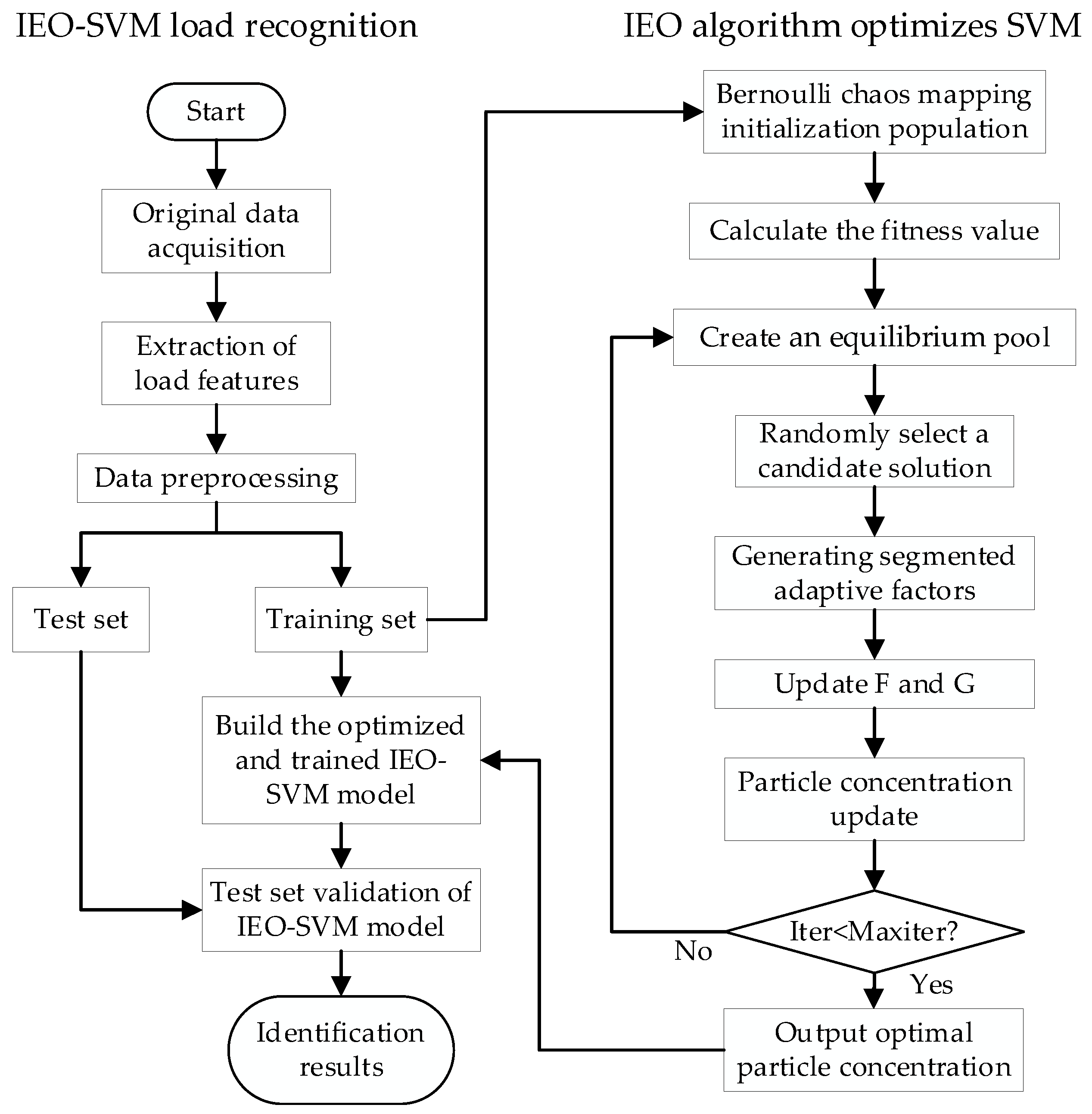
3.4. Load Identification Algorithm Based on IEO-SVM Model

In this paper, we propose a non-intrusive load identification method based on the IEO-SVM model as shown in Figure 4.

4. Dataset

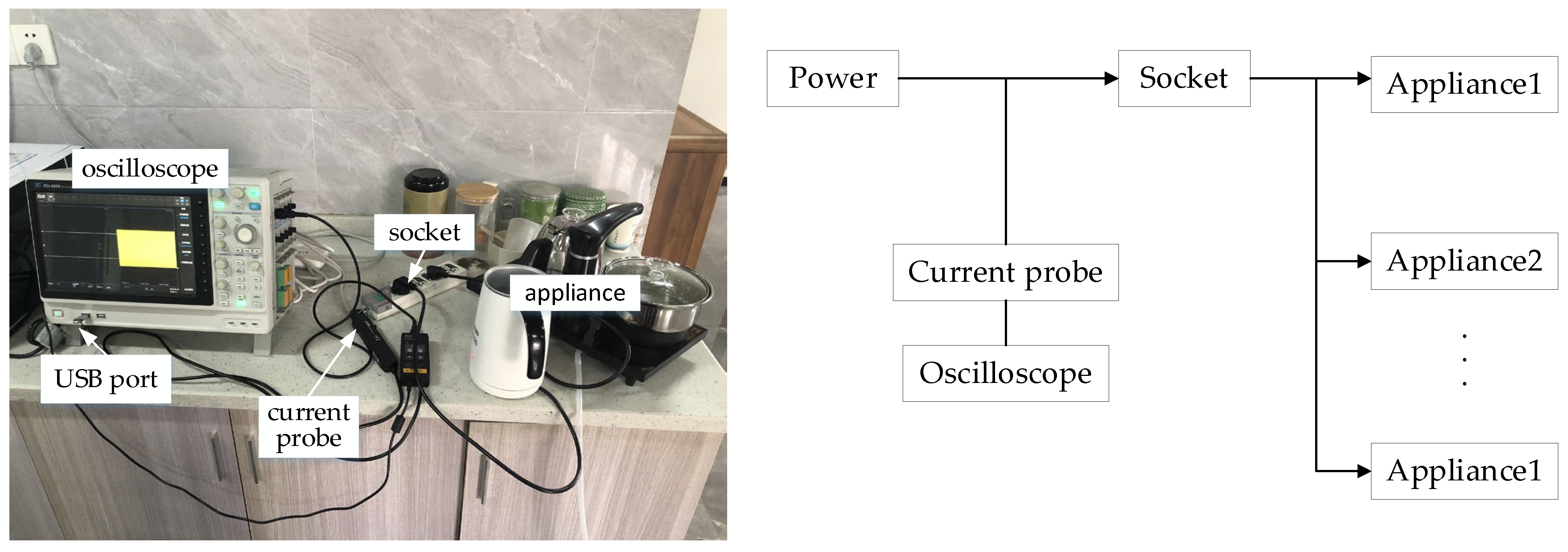
4.1. Self-Test Dataset

4.1.1. Raw Data Acquisition

To conduct experimental verification, data acquisition was performed on household appliances under laboratory conditions. The data acquisition device employed the ZDL6000 oscilloscope recorder and ZCP30 current probe, with a power supply of 200 V 50 Hz AC. The data acquisition device and the connection diagram are shown in Figure 5.

Plug the appliance into the socket and energize it, then clip the current probe of the oscilloscope to the incoming end of the socket, set the sampling frequency to 50 KHz to quickly collect the sample high-frequency data, and at the same time, plug the U disk into the USB port of the oscilloscope to save the data on the U disk in the .mat format, and send the data to the computer side for data analysis through the U disk. The data of 14 household appliance loads such as smartphones, laptops, microwave ovens (both running and standby states) and combined appliances were collected in a laboratory environment based on the data acquisition device. The categories are shown in

Table 1. Measured single electrical appliance and combined electrical appliance categories.

Electrical Appliance Category	Electrical Appliance Category
Smartphone	Desktop computer
Laptop	Tablet PC + Desktop computer
Induction cooker (standby)	Induction cooker (running) + Microwave oven (running)
Induction cooker (running)	Induction cooker (running) + Smartphone
Microwave oven (standby)	Microwave oven (running) + Smartphone
Microwave oven (running)	Microwave oven (running) + Tablet PC
Coffee maker	Smartphone + Laptop

. The current waveforms for each appliance within three cycles are shown in Figure 6.

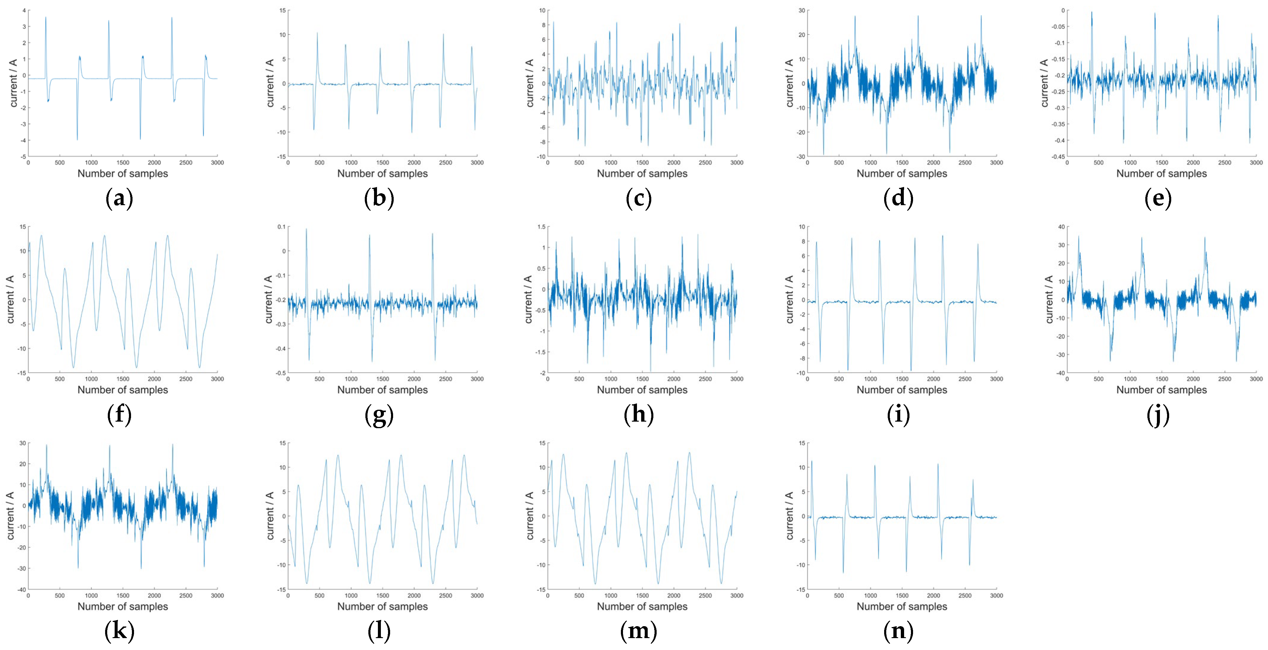
4.1.2. Dataset Production

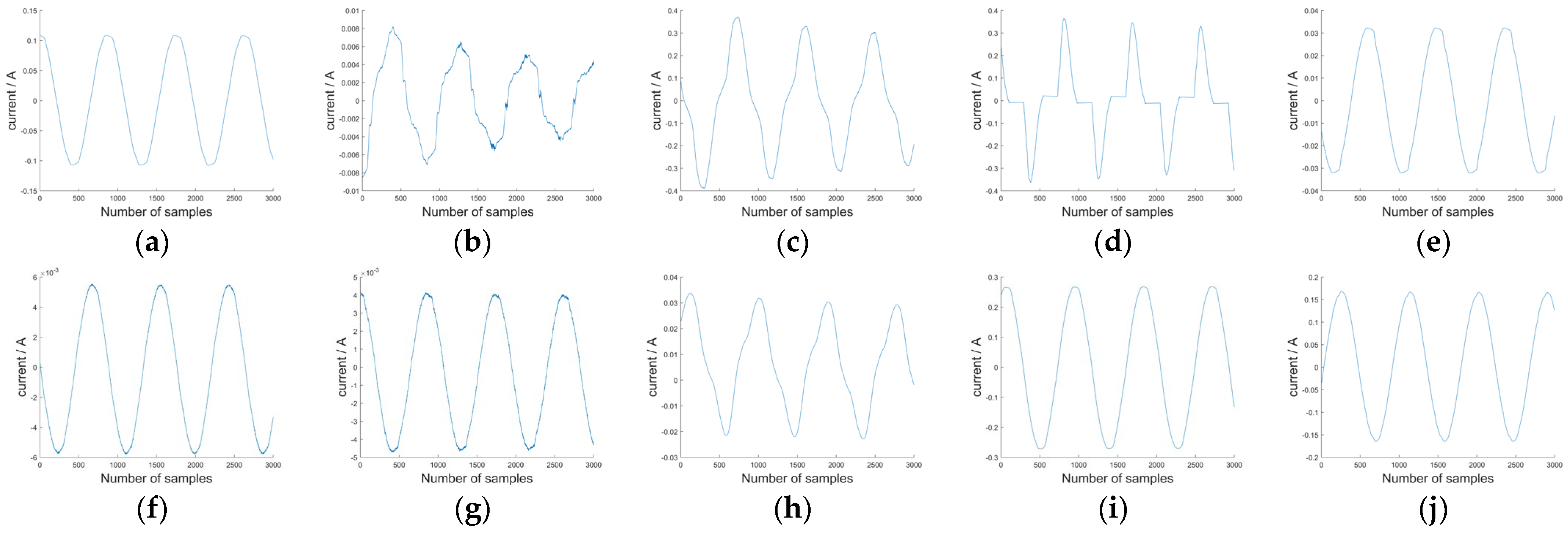
Each appliance category is sampled for 20 s, which corresponds to 1000 cycles, with 1000 sampling points per cycle, and the data of each cycle is the sample data. The corresponding labels for each appliance are set as shown in

Table 2. The labels corresponding to the appliance categories.

Electrical Appliance Category	Label	Electrical Appliance Category	Label
Smartphone	1	Desktop computer	8
Laptop	2	Tablet PC + Desktop computer	9
Induction cooker (standby)	3	Induction cooker (running) + Microwave oven (running)	10
Induction cooker (running)	4	Induction cooker (running) + Smartphone	11
Microwave oven (standby)	5	Microwave oven (running) + Smartphone	12
Microwave oven (running)	6	Microwave oven (running) + Tablet PC	13
Coffee maker	7	Smartphone + Laptop	14

. Seven load features such as $I_{peak}$, $I_{avg}$, $I_{\mathrm{var}}$, $I_{rms}$ and the 1st, 3rd and 5th current harmonic amplitudes are extracted from the original current data of each appliance category in turn in terms of cycles. Then, the extracted load features data are normalized, and the self-test data acquisition and processing are finished. There are 14,000 sample data for 14 types of appliances, of which 90% are the training set and 10% are the test set.

4.2. Public Dataset

To increase the diversity of the data, testing was conducted not only using a self-test dataset but also the WHITED dataset [36]. The WHITED dataset includes 47 different types of appliance categories from 6 different regions, with a sampling frequency of 44.1KHz and each cycle consisting of 882 data points. We selected 10 appliances from the WHITED dataset, including appliances from different brands. The 10 appliance categories ([Category]_[brand]) and their corresponding labels are shown in

Table 3. The appliance types and labels in the WHITED dataset.

Electrical Appliance Category	Label
WaterHeater_Daalderop	1
WashingMachine_Privileg	2
VacuumCleaner_Vento	3
VacuumCleaner_Nilfisk	4
RiceCooker_PanasonicSRG06	5
Fan_VOV-50W	6
LightBulb_Vintage-40W	7
KitchenHood_AmicaUH17051	8
Kettle_TCM	9
Hairdryer_Valera54206	10

. The current waveform is shown in Figure 7. The extraction and preprocessing of load features, as well as the data partitioning, were carried out using the same procedures as those applied to the self-collected dataset.

5. Experimental Analysis and Discussion

The data analysis in this paper is all based on Asus FX50VX PC with i7-6700HQ CPU, 2.60 GHz, 12G RAM, 512 GB hard disk, OS: Windows 10, and the compiled environment used is Python 3.7.

5.1. Experimental Design and Evaluation Metrics

To validate the effectiveness of the proposed method, we compared the following 11 approaches, including machine learning algorithms and existing deep learning algorithms.

(1)

IEO-SVM: the proposed method in this paper.

(2)

EO-SVM: the SVM method is optimized by the original EO algorithm.

(3)

SVM: support vector machine

(4)

LR: logistic regression

(5)

ANN: artificial neural network

(6)

DT: decision tree

(7)

k-NN: k-nearest neighbor

(8)

PSO-SVM: the method based on PSO-SVM used in reference [20].

(9)

AlexNet: the method based on the AlexNet deep learning model used in reference [13].

(10)

CNN: the novel structural convolutional neural network method used in reference [23].

(11)

CNN-LSTM: the method based on the CNN-LSTM deep learning model used in reference [27].

Due to the differences in the datasets and processing methods used in existing approaches, these disparities can lead to abnormal result comparisons. Therefore, we only utilize their core methods while keeping other experimental settings unchanged. We designed three experiments as follows. The experimental procedure is based on the load identification process outlined in Section 3.4, where different methods only differ in the recognition method used during the training of the model, while the remaining steps remain the same. It is worth noting that the first experiment is only conducted to validate the optimization capability of the proposed improved equilibrium optimizer algorithm and does not involve a comparison with the above load identification methods.

(1)

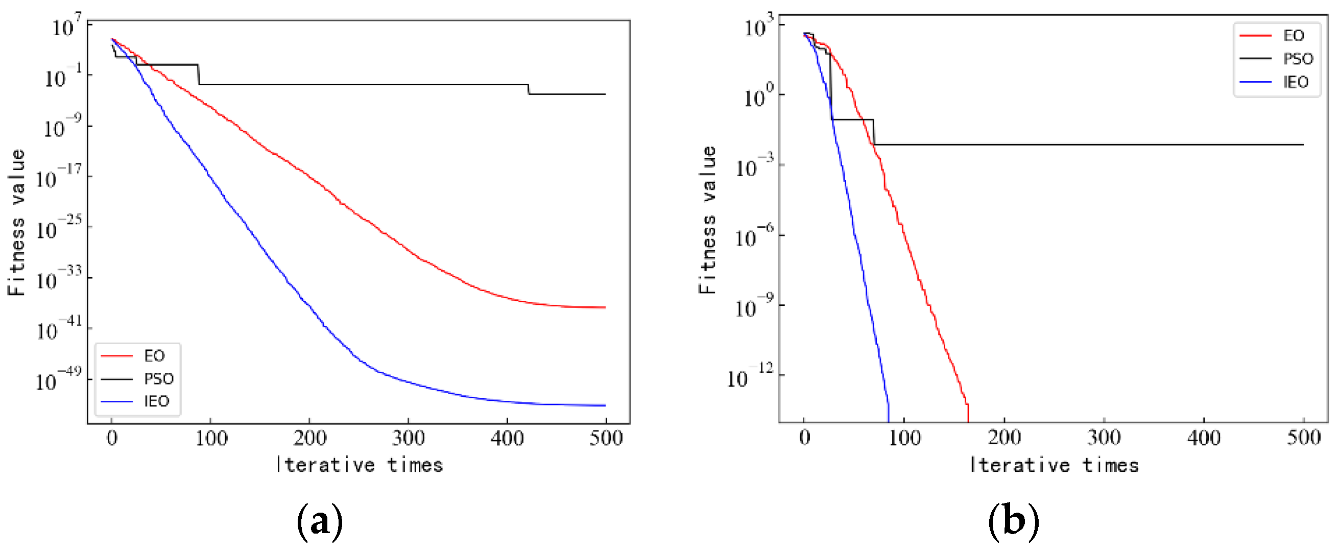
Experiment 1: The proposed IEO algorithm is compared and analyzed with EO and PSO algorithms based on benchmark functions. The superiority of the proposed IEO algorithm is validated using the average of five optimization values and convergence curves of the algorithm.

(2)

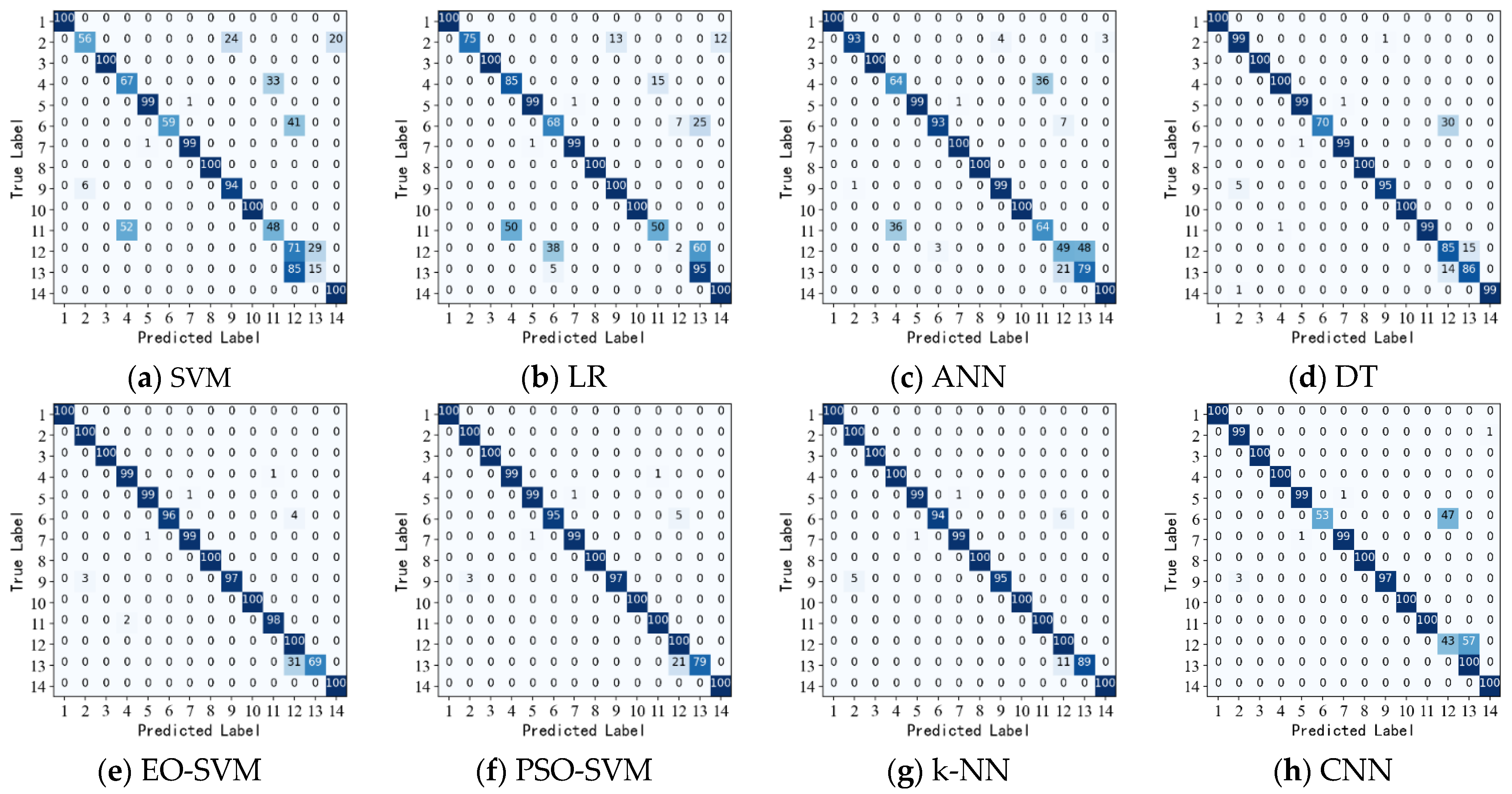
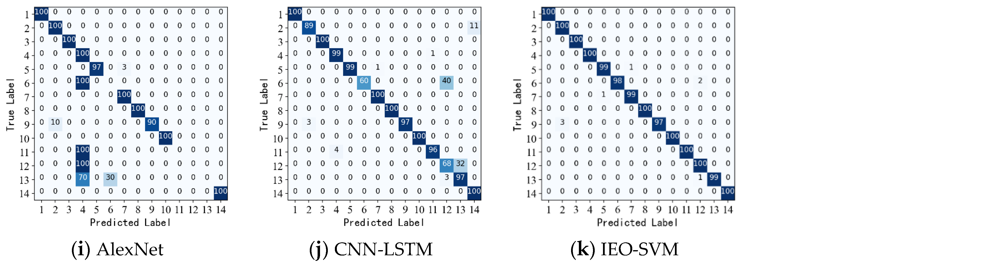
Experiment 2: The proposed IEO-SVM method is compared with other load identification algorithms using a self-test dataset. The experimental results are analyzed using a confusion matrix and four evaluation metrics (accuracy, precision, recall and F1_score).

(3)

Experiment 3: The IEO-SVM method is compared with other methods using a publicly available dataset. The results are analyzed using four evaluation metrics (accuracy, precision, recall and F1_score).

Accuracy, precision, recall and F1_score are commonly used to indicate the classification performance of load identification methods. The calculation formulas for the four metrics are shown as follows.

$$Accuracy=\frac{1}{n}{\displaystyle \sum _{i=1}^n\frac{T{P}_i+T{N}_i}{T{P}_i+T{N}_i+F{P}_i+F{N}_i}}$$

(27)

$$Precision=\frac{1}{n}{\displaystyle \sum _{i=1}^n\frac{T{P}_i}{T{P}_i+F{P}_i}}$$

(28)

$$Recall=\frac{1}{n}{\displaystyle \sum _{i=1}^n\frac{T{P}_i}{T{P}_i+F{N}_i}}$$

(29)

$$F1\_value=\frac{1}{n}{\displaystyle \sum _{i=1}^n\frac{2T{P}_i}{2T{P}_i+F{P}_i+F{N}_i}}$$

(30)

5.2. IEO Algorithm Performance Test

To test the effectiveness and the performance of the IEO algorithm, this paper selects seven benchmark test functions for validation purposes, of which $f_1\sim f_4$ refer to high-dimensional single-peak test functions used to evaluate the algorithm’s local exploitation capability and $f_5\sim f_7$ represent high-dimensional multi-peak test functions utilized to assess the algorithm’s global search ability and its capacity to escape local optima. The IEO algorithm is compared with the EO and PSO [16] by calculating seven test functions. To maintain fairness in comparing the algorithms, the parameters are set uniformly as follows: the population size is fixed at 30, the maximum number of iterations is set to 500, and the dimension is set to 30. The average of five search results is selected as the evaluation index, and the search results of the IEO algorithm are bolded. The results are shown in

Table 4. Comparison of the results of the test functions.

Function Name and Expression	Dimension	Algorithm	Search Space	Theoretical Optimal Value	The Average of Five Results
Sphere: $f_1={\displaystyle \sum _{i=1}^n{x}_i{}^2}$	30	EO	[−100, 100]	0	3.2835 × 10−39
		PSO		0	3.0278 × 10−2
		IEO		0	4.8112 × 10−54
Schwefel2.22: $f_2={\displaystyle \sum _{i=1}^n\left|x_i\right|}+{\displaystyle \prod _{i=1}^n\left|x_i\right|}$	30	EO	[−10, 10]	0	2.7620 × 10−23
		PSO		0	1.3831 × 10−1
		IEO		0	2.9701 × 10−32
Schwefel1.2: $f_3={\displaystyle \sum _{i=1}^n{({\displaystyle \sum _{j-1}^i{x}_j})}^2}$	30	EO	[−100, 100]	0	6.1848 × 10−8
		PSO		0	6.6840 × 101
		IEO		0	9.3542 × 10−21
Schwefel2.21: $f_4={\max }_i\{\left|x_i\right|,1\le i\le n\}$	30	EO	[−10, 10]	0	4.1181 × 10−10
		PSO		0	1.2619 × 10−2
		IEO		0	1.1893 × 10−18
Rastrigin: $f_5={\displaystyle \sum _{i=1}^n(x_i{}^2-10\cos (2\pi x_i)+10)}$	30	EO	[−5.12, 5.12]	0	0
		PSO		0	3.4332 × 10−3
		IEO		0	0
Ackley: $\begin{array}{l}{f}_6=-20\exp (-0.2\sqrt{\frac{1}{n}{\displaystyle \sum _{i=1}^n{x}_i{}^2}})\\ -\exp (\frac{1}{n}{\displaystyle \sum _{i=1}^n\cos (2\pi x_i)})+20+e\end{array}$	30	EO	[−32, 32]	0	7.5495 × 10−15
		PSO		0	1.3490 × 10−1
		IEO		0	3.9968 × 10−15
Griewank: $f_7=\frac{1}{4000}{\displaystyle \sum _{i=1}^n{x}_i{}^2}-{\displaystyle \prod _{i=1}^n\cos (\frac{x_i}{\sqrt{i}})+1}$	30	EO	[−600, 600]	0	0
		PSO		0	5.0186 × 10−2
		IEO		0	0

. From Table 4, the search accuracy of the IEO algorithm is significantly higher than that of the EO algorithm and the PSO algorithm, and it is higher by a certain order of magnitude, while for $f_5$ and $f_7$, the IEO algorithm can search for the optimal value within the search space, and the search effect is outstanding. As a result, the IEO algorithm with the improved strategy exhibits a superior search performance.

To visually observe the optimization accuracy and convergence speed of the IEO algorithm, this paper plots the convergence curves of several test functions using the number of iterations and corresponding fitness values. The results are shown in Figure 8. By observing the convergence curves of some test functions, the IEO algorithm converges late, overcoming the problem of premature convergence of other algorithms, and also shows a greater advantage in search accuracy and convergence speed. Therefore, the IEO algorithm can effectively improve the population quality and quickly jump out of the local optimum with high adaptability.

5.3. Analysis of the Results on the Self-Test Dataset

This section conducts experiments based on the self-test dataset. There are a total of 14 appliances with 14,000 samples, including 12,600 training samples and 1400 testing samples. The classification results are visually analyzed by drawing the confusion matrix to facilitate the observation of the recognition effect of each algorithm.

The confusion matrix is plotted as shown in Figure 9, where the horizontal axis is the predicted labels of appliance categories, and the vertical axis is the actual labels of appliance categories. Each element in the confusion matrix represents the number of vertical-axis appliance categories predicted to be horizontal-axis appliance categories. Analyzing the confusion matrix, it is found that the traditional SVM algorithm and the LR algorithm are less effective in recognition and have too many recognition errors for most of the appliances. The problem with the traditional SVM algorithm is mainly that its parameter selection depends on experience and there is no guarantee that the selected parameters are optimal. The LR algorithm mainly solves the linear problem, and the poor recognition effect indicates that the sample data are nonlinear and therefore cannot be recognized effectively. For the ANN and DT algorithms, the main focus is on the misidentification between three groups of appliance categories, category 4 (induction cooker (running)) and category 11 (induction cooker (running) + smartphone), category 12 (microwave oven (running) + smartphone) and category 13 (microwave oven (running) + tablet PC), and category 6 (microwave oven (running)) and category 12, which are all high-current appliances covering small-current appliances (the stable operating current of an induction cooker and microwave oven is greater than the current of a smartphone and tablet PC). So, the ANN and LR algorithms cannot accurately identify such appliances. The error recognition of the CNN and CNN-LSTM algorithms is mainly concentrated in categories 6 and 12, and they are also unable to effectively identify loads of this type. The AlexNet algorithm exhibits low classification performance due to severe overfitting. Although the EO-SVM, PSO-SVM, and k-NN algorithms have a better recognition effect for the two groups of appliances, categories 4 and 11, and categories 6 and 12, they still cannot effectively recognize for categories 12 and 13, which is because the EO and PSO algorithms very easily fall into the local optimum in the process of optimizing the SVM and cannot seek the optimal SVM, resulting in slightly poor recognition, while the k-NN algorithm needs to be built based on sample balance for recognition. The IEO-SVM algorithm proposed in this paper improves the recognition effect of high-current covering small-current appliances compared with other algorithms and maintains good load recognition for other appliances. The IEO-SVM algorithm surpasses other methods and overcomes the issue of local optimization encountered by the EO and PSO algorithms during the SVM optimization process. It ensures the optimality of the SVM model and effectively improves the performance of the model. Furthermore, the IEO-SVM model achieves higher recognition accuracy.

The evaluation metric results for each method are shown in

Table 5. Experimental results of self-test dataset.

Evaluation Metrics	Accuracy	Precision	Recall	F1_Value
SVM	79.14%	81.22%	79.14%	78.67%
LR	83.79%	82.28%	83.78%	81.49%
ANN	88.57%	88.7%	88.57%	88.49%
DT	95.07%	95.81%	95.07%	95.16%
EO-SVM	96.93%	97.58%	96.93%	96.91%
PSO-SVM [20]	97.71%	98.1%	97.71%	97.73%
k-NN	98.29%	98.48%	98.28%	98.3%
CNN [23]	92.14%	93.25%	92.14%	91.88%
AlexNet [13]	70.5%	64.95%	70.5%	68.86%
CNN-LSTM [27]	93.21%	94.1%	93.2%	93.15%
IEO-SVM	99.43%	99.44%	99.42%	99.43%

. From Table 5, it can be observed that the IEO-SVM method exhibits the highest recognition accuracy, which is 99.43%. Compared to SVM, LR, ANN, DT, EO-SVM, PSO-SVM, k-NN, CNN, AlexNet and CNN-LSTM, the recognition accuracy of our proposed method has been improved by 20.29%, 15.64%, 10.86%, 4.36%, 2.5%, 1.72%, 1.14%, 7.29%, 28.93% and 6.22%, respectively. The IEO-SM model improves the precision, recall, and F1_ value on all three evaluation metrics. The results indicate that the IEO-SVM method is capable of handling recognition tasks on self-evaluation datasets, demonstrating a high level of recognition accuracy and classification performance.

5.4. Analysis of the Results on the Public Dataset

Experiments in this section were conducted based on the WHITED dataset. There are a total of 10 appliances with 10,000 samples, including 9000 training samples and 1000 testing samples. The classification results are analyzed using evaluation metrics, using accuracy to assess the overall classification performance of the methods.

From

Table 6. Experimental results of WHITED dataset.

Evaluation Metrics	Accuracy	Precision	Recall	F1_Value
SVM	89%	93.95%	89%	85.9%
LR	70.9%	66.15%	70.8%	65.7%
ANN	69.7%	77.18%	69.7%	66.16%
DT	100%	100%	100%	100%
EO-SVM	94.9%	96.62%	94.9%	94.54%
PSO-SVM [20]	95.8%	97.04%	95.8%	95.6%
k-NN	100%	100%	100%	100%
CNN [23]	81.5%	75.97%	81.5%	77.63%
AlexNet [13]	74.7%	70.37%	74.7%	71%
CNN-LSTM [27]	98.3%	98.44%	98.3%	98.29%
IEO-SVM	100%	100%	100%	100%

, it can be seen that the IEO-SVM method exhibits superior classification performance. It is worth noting that the accuracy on the WHITED dataset reached 100%. Among other machine learning algorithms, the DT and k-NN methods also exhibit a good recognition performance. Among the existing deep learning algorithms, the CNN and AlexNet methods suffer from a poor recognition performance due to overfitting issues. The CNN-LSTM method shows better overall classification performance, but compared to the IEO-SVM method, there is still room for improvement in terms of accuracy. The results indicate that the overall classification performance of the IEO-SVM method is superior to other methods on the WHITED dataset.

5.5. Feasibility Analysis of the IEO-SVM Method

Based on the above results and discussions, the IEO-SVM method performs well on both the self-test dataset and the WHITED dataset. Although the DT, k-NN and CNN-LSTM methods perform well on the WHITED dataset, there is still a gap compared to the IEO-SVM method on the self-test dataset. This indicates that the IEO-SVM method can not only handle appliance recognition tasks in public datasets but also handle specialized appliance recognition tasks in the self-test dataset, such as identifying high-current appliances that overlap with low-current appliances. Due to its excellent classification performance, the IEO-SVM method can achieve more accurate identification of appliances and can be better applied in practical scenarios.

6. Conclusions

In this paper, we propose an improved EO algorithm to optimize the load identification algorithm of the SVM for the problem of difficult parameter selection when the SVM is performing load identification tasks. When performing load identification tasks based on the IEO-SVM model, the standard EO algorithm is improved by using Bernoulli chaotic sequences to initialize the population, dynamic adjustment parameters, and Levy flight perturbation concentration update strategy. Based on the testing functions, the IEO algorithm demonstrates good optimization performance with fast convergence speed and high convergence accuracy, establishing an IEO-SVM load identification model and validating it based on both a self-test dataset and a public dataset (WHITED). The results demonstrate that the IEO-SVM method significantly improves the recognition accuracy in both datasets. It can better address the challenge of distinguishing between appliances with a high current and those with a low current in the self-test dataset.

In the future, we need to consider the application in complex environments, as well as the deployment of the algorithm, while ensuring recognition accuracy, simplifying the model and reducing time costs.

References

1. Lee, H. Towards Convergence in Federated Learning via Non-IID Analysis in a Distributed Solar Energy Grid. Electronics 2023, 12, 1580. [Google Scholar] [CrossRef]
2. Liaqat, R.; Sajjad, I.A. An Event Matching Energy Disaggregation Algorithm Using Smart Meter Data. Electronics 2022, 11, 3596. [Google Scholar] [CrossRef]
3. Yang, M.; Li, X.; Liu, Y. Sequence to Point Learning Based on an Attention Neural Network for Nonintrusive Load Decomposition. Electronics 2021, 10, 1657. [Google Scholar] [CrossRef]
4. Zoha, A.; Gluhak, A.; Imran, M.A.; Rajasegarar, S. Non-intrusive load monitoring approaches for disaggregated energy sensing: A survey. Sensors 2012, 12, 16838–16866. [Google Scholar] [CrossRef] [Green Version]
5. Chui, K.T.; Hung, F.H.; Li, B.Y.S.; Tsang, K.F.; Chung, H.S. Appliance signature: Multi-modes electric appliances. In Proceedings of the 2014 IEEE International Conference on Consumer Electronics, Shenzhen, China, 9–13 April 2014; pp. 1–3. [Google Scholar]
6. Lemes, D.A.M.; Cabral, T.W.; Fraidenraich, G.; Meloni, L.G.P.; Lima, E.R.D.L.; Neto, F.B. Load disaggregation based on time window for HEMS application. IEEE Access 2021, 9, 70746–70757. [Google Scholar] [CrossRef]
7. Salerno, V.M.; Rabbeni, G. An Extreme Learning Machine Approach to Effective Energy Disaggregation. Electronics 2018, 7, 235. [Google Scholar] [CrossRef] [Green Version]
8. Chang, H.; Lin, L.; Chen, N.; Lee, W. Particle-Swarm-Optimization-Based Nonintrusive Demand Monitoring and Load Identification in Smart Meters. IEEE Trans. Ind. Appl. 2013, 49, 2229–2236. [Google Scholar] [CrossRef]
9. Chea, R.; Thourn, K.; Chhorn, S. Improving VI Trajectory Load Signature in NILM Approach. In Proceedings of the 2022 International Electrical Engineering Congress, Khon Kaen, Thailand, 9–11 March 2022; pp. 1–4. [Google Scholar]
10. Abraham, O.A.; Ochiai, H.; Shibly, K.H.; Hossain, M.D.; Taenaka, Y.; Kadobayashi, Y. Unauthorized Power Usage Detection Using Gradient Boosting Classifier in Disaggregated Smart Meter Home Network. In Proceedings of the 2022 IEEE Future Networks World Forum, Montreal, QC, Canada, 10–14 October 2022; pp. 688–693. [Google Scholar]
11. Kramer, O.; Klingenberg, T.; Sonnenschein, M.; Wilken, O. Non-intrusive appliance load monitoring with bagging classifiers. Log. J. IGPL 2015, 23, 359–368. [Google Scholar] [CrossRef]
12. Gillis, J.M.; Alshareef, S.M.; Morsi, W.G. Nonintrusive load monitoring using wavelet design and machine learning. IEEE Trans. Smart Grid 2015, 7, 320–328. [Google Scholar] [CrossRef]
13. Liu, Y.; Wang, X.; You, W. Non-intrusive load monitoring by voltage–current trajectory enabled transfer learning. IEEE Trans. Smart Grid 2018, 10, 5609–5619. [Google Scholar] [CrossRef]
14. Chang, H.; Lee, M.; Lee, W.; Chien, C.; Chen, N. Feature Extraction-Based Hellinger Distance Algorithm for Nonintrusive Aging Load Identification in Residential Buildings. IEEE Trans. Ind. Appl. 2016, 52, 2031–2039. [Google Scholar] [CrossRef]
15. Chen, T.; Qin, H.; Li, X.; Wan, W.; Yan, W. A Non-Intrusive Load Monitoring Method Based on Feature Fusion and SE-ResNet. Electronics 2023, 12, 1909. [Google Scholar] [CrossRef]
16. Mahmudur Rahman Khan, M.; Siddique, A.B.; Sakib, S. Non-Intrusive Electrical Appliances Monitoring and Classification using K-Nearest Neighbors. In Proceedings of the 2019 2nd International Conference on Innovation in Engineering and Technology, Dhaka, Bangladesh, 23–24 December 2019; pp. 1–5. [Google Scholar]
17. Su, S.; Yan, Y.; Lu, H.; Li, K.; Sun, Y.; Wang, F.; Liu, L.; Ren, H. Non-intrusive load monitoring of air conditioning using low-resolution smart meter data. In Proceedings of the 2016 IEEE International Conference on Power System Technology, Wollongong, NSW, Australia, 28 September–1 October 2016; pp. 1–5. [Google Scholar]
18. Dufour, L.; Genoud, D.; Jara, A.; Treboux, J.; Ladevie, B.; Bezian, J. A non-intrusive model to predict the exible energy in a residential building. In Proceedings of the 2015 IEEE Wireless Communications and Networking Conference Workshops, New Orleans, LA, USA, 9–12 March 2015; pp. 69–74. [Google Scholar]
19. Su, D.; Shi, Q.; Xu, H.; Wang, W. Nonintrusive load monitoring based on complementary features of spurious emissions. Electronics 2019, 8, 1002. [Google Scholar] [CrossRef] [Green Version]
20. Gong, F.; Han, N.; Zhou, Y.; Chen, S.; Li, D.; Tian, S. A svm optimized by particle swarm optimization approach to load disaggregation in non-intrusive load monitoring in smart homes. In Proceedings of the 2019 IEEE 3rd Conference on Energy Internet and Energy System Integration, Changsha, China, 8–10 November 2019; pp. 1793–1797. [Google Scholar]
21. Liu, K.; Fu, Y.; Wang, P.; Wu, L.; Bo, R.; Li, X. Automating feature subspace exploration via multi-agent reinforcement learning. In Proceedings of the 25th ACM SIGKDD International Conference on Knowledge Discovery, New York, NY, USA, 4–8 August 2019; pp. 207–215. [Google Scholar]
22. Kolter, J.Z.; Jaakkola, T. Approximate inference in additive factorial hmms with application to energy disaggregation. In Proceedings of the Fifteenth International Conference on Artificial Intelligence and Statistics, La Palma, Canary Islands, Spain, 21–23 April 2012; pp. 1472–1482. [Google Scholar]
23. Zhou, Y.; Shi, Z.; Shi, Z.; Gao, Q.; Wu, L. Disaggregating power consumption of commercial buildings based on the finite mixture model. Appl. Energy 2019, 243, 35–46. [Google Scholar] [CrossRef]
24. Ciancetta, F.; Bucci, G.; Fiorucci, E.; Mari, S.; Fioravanti, A. A new convolutional neural network-based system for NILM applications. IEEE Trans. Instrum. Meas. 2020, 70, 1501112. [Google Scholar] [CrossRef]
25. Guo, L.; Wang, S.; Chen, H.; Shi, Q. A load identification method based on active deep learning and discrete wavelet transform. IEEE Access 2020, 8, 113932–113942. [Google Scholar] [CrossRef]
26. Tian, Y.; Wang, H.; Li, A.; Shi, S.; Wu, J. Non-intrusive load monitoring using inception structure deep learning. In Proceedings of the 2020 10th International Conference on Power and Energy Systems (ICPES), Chengdu, China, 25–27 December 2020; pp. 151–155. [Google Scholar]
27. Du, L.; He, D.; Harley, R.G.; Habetler, T.G. Electric load classification by binary voltage–current trajectory mapping. IEEE Trans. Smart Grid 2015, 7, 358–365. [Google Scholar] [CrossRef]
28. Chen, C.; Gao, P.; Jiang, J.; Jiang, J.; Wang, H.; Li, P.; Wan, S. A deep learning based non-intrusive household load identification for smart grid in China. Comput. Commun. 2021, 177, 176–184. [Google Scholar] [CrossRef]
29. Kaselimi, M.; Doulamis, N.; Doulamis, A.; Voulodimos, A.; Protopapadakis, E. Bayesian-optimized bidirectional LSTM regression model for non-intrusive load monitoring. In Proceedings of the ICASSP 2019—2019 IEEE International Conference on Acoustics, Speech and Signal Processing (ICASSP), Brighton, UK, 12–17 May 2019; pp. 2747–2751. [Google Scholar]
30. Faramarzi, A.; Heidarinejad, M.; Stephens, B.; Mirjalili, S. Equilibrium optimizer: A novel optimization algorithm. Knowl.-Based Syst. 2020, 191, 105190. [Google Scholar] [CrossRef]
31. Kennedy, J.; Eberhart, R. Particle swarm optimization. In Proceedings of the ICNN’95-International Conference on Neural Networks, Perth, WA, Australia, 27 November–1 December 1995; pp. 1942–1948. [Google Scholar]
32. Kamaruzaman, A.F.; Zain, A.M.; Yusuf, S.M.; Udin, A. Levy flight algorithm for optimization problems-a literature review. Appl. Mech. Mater. 2013, 421, 496–501. [Google Scholar] [CrossRef]
33. Yan, B.; Zhao, Z.; Zhou, Y.; Yuan, W.; Li, J.; Wu, J.; Cheng, D. A particle swarm optimization algorithm with random learning mechanism and Levy flight for optimization of atomic clusters. Comput. Phys. Commun. 2017, 219, 79–86. [Google Scholar] [CrossRef]
34. Pathak, Y.; Arya, K.V.; Tiwari, S. Feature selection for image steganalysis using levy flight-based grey wolf optimization. Multimed. Tools Appl. 2019, 78, 1473–1494. [Google Scholar] [CrossRef]
35. Lopes, F.F.; Ferreira, J.C.; Fernandes, M.A. Parallel Implementation on FPGA of Support Vector Machines Using Stochastic Gradient Descent. Electronics 2019, 8, 631. [Google Scholar] [CrossRef] [Green Version]
36. Kahl, M.; Haq, A.U.; Kriechbaumer, T.; Jacobsen, H.A. WHITED—A Worldwide Household and Industry Transient Energy DataSet. In Proceedings of the 3rd International Workshop on Non-Intrusive Load Monitoring, Simon Fraser University, Vancouver, BC, Canada, 14–15 May 2016. [Google Scholar]
Figure 1. (a) Microwave oven (running state) current waveform and (b) laptop current waveform.
Electronics 12 03138 g001
Figure 2. Induction cooker (running state) spectrum chart.
Electronics 12 03138 g002
Figure 3. Levy flight path.
Electronics 12 03138 g003
Figure 4. Flow diagram of load identification algorithm based on IEO-SVM.
Electronics 12 03138 g004
Figure 5. Experimental acquisition device and connection diagram.
Electronics 12 03138 g005
Figure 6. Current waveforms of 14 electrical appliances: (a) Smartphone; (b) Laptop; (c) Induction cooker (standby); (d) Induction cooker (running); (e) Microwave oven (standby); (f) Microwave oven (running); (g) Coffee maker; (h) Desktop computer; (i) Tablet PC + Desktop computer; (j) Induction cooker (running) + Microwave oven (running); (k) Induction cooker (running) + Smartphone; (l) Microwave oven (running) + Smartphone; (m) Microwave oven (running) + Tablet PC; and (n) Smartphone + Laptop.
Electronics 12 03138 g006
Figure 7. Current waveforms of 10 electrical appliances: (a) WaterHeater; (b) WashingMachine; (c) VacuumCleaner_Vento; (d) VacuumCleaner_Nilfisk; (e) RiceCooker; (f) Fan; (g) LightBulb; (h) KitchenHood; (i) Kettle; and (j) Hairdryer.
Electronics 12 03138 g007
Figure 8. (a) Convergence diagram of f1 function, and (b) convergence diagram of f 5 function.
Electronics 12 03138 g008
Figure 9. The confusion matrix results for SVM, LR, ANN, DT, EO-SVM, PSO-SVM, k-NN, CNN, AlexNet, CNN-LSTM and IEO-SVM (ak).
Electronics 12 03138 g009aElectronics 12 03138 g009b