Interval Type 2 Fuzzy Adaptive Motion Drive Algorithm Design

Abstract

Motion drive algorithms are a set of filters designed to simulate realistic motion and are an integral part of contemporary vehicle simulators. This paper presents the design of a novel intelligent interval type 2 fuzzy adaptive motion drive algorithm for an off-road uphill vehicle simulator. The off-road, uphill vehicle simulator is used to train and assess the driver’s behavior under varying operational and environmental conditions in mountainous terrain. The proposed algorithm is the first of its kind to be proposed for off-road uphill vehicle simulators, and it offers numerous benefits over other motion drive algorithms. The proposed algorithm enables the simulator to adapt to changes in the uphill road surface, vehicle weight distribution, and other factors that influence off-road driving in mountainous terrain. The proposed algorithm simulates driving on hilly terrain more realistically than existing algorithms, allowing drivers to learn and practice in a safe and controlled environment. Additionally, the proposed algorithm overcomes limitations present in existing algorithms. The performance of the proposed algorithm is evaluated via test drives and compared to the performance of the conventional motion drive algorithm. The results demonstrate that the proposed algorithm is more effective than the conventional motion drive algorithm for the ground vehicle simulator. The pitch and roll responses demonstrate that the proposed algorithm has enabled the driver to experience abrupt changes in terrain while maintaining the driver’s safety. The surge response demonstrated that the proposed MDA handled the acceleration and deceleration of the vehicle very effectively. In addition, the results demonstrated that the proposed algorithm resulted in a smoother drive, prevented false motion cues, and offered a more immersive and realistic driving experience.

1. Introduction

Motion simulators were primarily developed for aircraft flight simulation. However, in the past few decades, the usage of motion simulators has increased in diversified fields and application domains, i.e., academia, aerial vehicle simulation and training, and driving vehicle simulation and training, among many. The increased popularity of motion simulators is due to the cost-effectiveness and safety features that it provides to simulate extreme conditions [1]. Like flight simulators, ground vehicle simulators have also gained popularity in the past few years. Ground vehicle simulators are employed for applications like driver training, driver behavior assessment, automotive research and manufacturing, and road accident analysis [2,3]. Typically, ground vehicle simulators are categorized as (i) driving (training) simulators and (ii) research simulators. Driving simulators provide the trainee drivers with an environment that emulates a real driving environment and allows the driver to drive the vehicle in various driving environments and conditions without using the actual vehicle. Thus, it enables the driver to fully master driving skills, learn driving regulations, and develop skills to effectively handle any possible emergencies. Furthermore, driving simulators are beneficial for use as compared to the real vehicle for testing or training in terms of saving time and cost-effectiveness by avoiding potential hazards such as accidents and vehicle failure and ensuring road safety. A considerable amount of work has been done on driving simulators; some of the important contributions in high-fidelity and intermediate-fidelity simulators are discussed below.

High-fidelity simulators provide the highest level of vehicle simulation with a broad field of view, realistic audio, visual, force feedback, and motion cues. These simulators are usually developed by automotive manufacturers for the testing and validation of new vehicles. Some notable high-fidelity simulators and their salient features are described in

Table 1. Summary of high-fidelity simulators.

Name	Initiation Year	Organization	Salient Features
VTI driving simulator [4]	1984	VTI Sweden	-8 DOF simulator -Traffic simulation -Exchangeable cabin design
Mercedes-Benz driving simulator [5,6,7]	1985	Mercedes Benz Germany	-7 DOF simulator (6 DOF platform + 12 m long rail) -360° projection screen
National advanced driving simulator (NADS-I) [8]	1996	University of Iowa USA	-13 DOF simulator -Large motion envelope -16 high-definition LED projector
Virttex simulator [9,10]	2000	Ford USA	-6 DOF simulator -45-megapixel, 360° projection screen -Exchangeable cabin design
The Ultimate Simulator [11,12]	2001	Renault Techno center	-8 DOF simulator (6 DOF platform, X and Y rails) -Panoramic screen -3D sound system
BMW driving simulator [13]	2003	BMW Germany	-6 DOF simulator -Dynamic car testing -Driving assistance system
UoLDS [14]	2006	University of Leeds UK	-8 DOF simulator (6DOF platform, XY table) -Jaguar S-type vehicle cab -3D graphics
Toyota driving simulator [15]	2007	Toyota Japan	-Largest driving simulator -Adjustable-speed generator to emulate the dangerous situation -360° spherical screen -realistic sound and motion
OKTAL simulator [16,17]	2011	Tongji University, China	-6 to 9 DOF motion platform -up to 360° visual screen -Total immersion
Stuttgart driving simulator [18,19]	2012	FKFS, Uni. of Stuttgart Germany	-8 DOF simulator (6 DOF platform, XY table) -Driver assistance system

.

Intermediate-fidelity simulators are simpler and more cost-effective as compared to high-fidelity simulators. These simulators use a partial or generalized cabin instead of perfect vehicle imitation but produce high-quality audio, visual, and motion cues. Some notable intermediate-fidelity simulators and their salient features are described in

Table 2. Summary of intermediate-fidelity simulators.

Name	Initiation Year	Organization	Salient Features
UCF driving simulator [20,21]	2002	University of Central Florida USA	-6 DOF simulator -180° of the field of view -3D road surface model -Traffic safety and operation analysis
DLR dynamic driving simulator [22]	2004	German Aerospace Center Germany	-6 DOF simulator -Inverted Cabin design -Large field-of-view projection system
Universal driving simulator [23]	2004	University of Tokyo Japan	-6 DOF simulator -360° of the field of view -Developed for drivers’ characteristics analysis
Chalmers vehicle simulator [24,25]	2005	Chalmers University of Technology Sweden	-6 DOF simulator -veDYNA model-based vehicle dynamic simulation
MPI CyberMotion Simulator [26]	2007	Max Planck Institute Germany	-7 DOF simulator -Anthropomorphic manipulator-based design
CARRS-Q Advanced Driving Simulator [27]	2011	Queensland University of Technology, Australia	-6 DOF simulator -Holden Commodore vehicle with instruments -For road safety research
Jaguar Land Rover simulator [28]	2012	Cruden Netherlands	-6 DOF simulator -Support design and test of Jaguar and Land Rover

.

The majority of existing driving simulators have focused on urban driving training and little attention is paid to off-road uphill driving simulators. Driving in hilly and mountainous areas is riskier and the accident rate in hilly areas is high as compared to urban areas due to road dynamics and driving behavior [29]. Therefore, there is a genuine need for the development of an off-road uphill driving simulator for driver training as well as testing for different road scenarios to avoid accidents.

The motion drive algorithm (MDA) or washout filter is an integral part of vehicle simulators. The MDA aims to replicate, as closely as possible, the motion of a real vehicle using a multi-degree-of-freedom motion platform. However, due to the limited movement of platform actuators, an exact rendering of the real vehicle’s motion is not possible. Therefore, MDA uses a set of low-pass filters (LPFs) and high-pass filters (HPFs) to produce motion within the platform motion envelope, allowing the user to have a realistic driving or flying experience. There are five major variations of MDA, which are referred to as (i) classical, (ii) adaptive, (iii) intelligent, (iv) optimal, and (v) hybrid, respectively. Conrad and Schmidt [30] conducted experiments that resulted in the development of classic washout filters as the most prevalent and cost-effective MDA. It is made up of a chain of HPF and LPF, and it also has an optional tilt coordination element. The tilt coordination generates continuous accelerations using lower frequencies of the vehicle data. The motion platform’s movement within its motion envelope is facilitated by the utilization of the higher-frequency elements of the motion data through the implementation of a high-pass filter. The classical washout filter has several benefits, including good efficiency, minimal computational cost, and ease of implementation. The classical washout filter is designed to make sure that the motion platform is always contained within the motion envelope. This assumption diminishes the algorithm’s ability to reproduce precise motion sensations. In addition to these problems, classical washout filters have other issues, such as fixed filters’ transfer function, neglecting the sensory model, and motion platform constraints. As a result of these limitations, motion sickness emerges as the most significant disadvantage of the MDA.

Parrish et al. [31] proposed the idea of the adaptive washout filter with variable cutoff frequencies of LPF and HPF. Reid and Nahon [32] used the coordinated adaptive washout filter to try to reduce the differences between how the real driver of the vehicle and the motion platform driver felt the motion. Nehaoua et al. [33,34] proposed an adaptive washout filter for a two-degrees-of-freedom (2-DoF) platform. They used the gradient descent (GD) technique to find the best values for HPF and LPF coefficients using error data and motion envelope constraints. Inayat et al. [35] proposed an adaptive washout filter for aircraft Hardware-In-the-Loop (HIL) simulation. Liao et al. [36] proposed a novel washout filter design in which they combined conventional and adaptive washout filters.

Fuzzy logic has been used by Hwang et al. [37] to modify the washout filters’ coefficients during operation to provide precise motion sensations. Asadi et al. [38] employed fuzzy logic to modify the cut-off frequencies of low- and high-pass filters, taking into account the differences in motion perception between the drivers of the actual vehicle and motion platform, in addition to the translational and rotational displacement of the motion platform. Although the provided technique proved effective for the six-degree-of-freedom (6DOF) Stewart platform, it is hindered by the need to account for the motion platform’s restriction in the Cartesian space for serial motion platforms. Asadi et al. [39] also offered a new feature of the adaptive washout filter that generates stabilized motion in response to changes in the current state of the platform, such as the end-deviation effectors from the equilibrium point.

Huang and Fu [40] proposed an optimal washout filter that relies on the Human Vestibular Model (HVM) and the constraints of the motion platform. The filter’s cost function was minimized by utilizing the driver sensation error, which was calculated by comparing the simulator and vehicle. In order to create realistic behavior, Chen and Fu [41] also proposed an optimal washout filter that accounts for the motion platform’s limited workspace and attempts to reduce human perception mistakes. Qazani et al. [42] have recently proposed an optimal washout filter using fuzzy and neural network-based system. While the neural network is implemented to solve the Riccati problem, the fuzzy logic model is developed to extract the weighting matrices used by the LQR approach. The suggested approach takes the physical limits of the motion platform into account in real time and produces a motion profile with a high degree of accuracy.

This study employs an Interval Type 2 (IT2) fuzzy-based adaptive MDA while considering the dynamic and physical features of the motion platform. IT2 fuzzy-based adaptive MDA is proposed for two reasons. To begin, IT2 fuzzy systems excel in dealing with uncertainty and imprecision [43,44]. Uncertainties in mountainous terrain include unexpected road conditions, variable slopes, and uneven traction. When paired with IT2 fuzzy systems, the adaptive nature of MDA allows the simulator to dynamically alter its settings based on changing terrain and vehicle circumstances. This versatility guarantees that the simulator can adjust to changes in the uphill road surface, vehicle weight distribution, and other aspects affecting off-road driving in mountainous terrain. Second, the simulator delivers a more immersive and realistic driving experience by merging IT2 fuzzy systems with adaptive MDA. The MDA can smooth out inputs and outputs, minimizing noise and vibrations caused by off-road driving. This results in a more accurate simulation of genuine mountain driving conditions, allowing drivers to gain significant experience and abilities in a controlled and safe setting. The secondary objective of the proposed algorithm is to solve the shortcomings of the current adaptive MDAs, for instance, overlooking the effect of sudden changes in angular velocities, which often happens in off-road simulators. The suggested MDA observes the velocities of the motion platform, as well as the driving perception error, in an effort to provide the correct motion data. This is to remedy the poor utilization of the motion envelope, which is a limitation for the vehicle simulator driver. The fuzzy IT2 controllers are employed to determine the proper cut-off frequencies for the HPFs and LPFs in the adaptive washout filter. The algorithm is tested using an indigenously developed off-road uphill vehicle simulator mounted on the Stewart platform. The efficacy of our proposed algorithm is assessed through a comparative analysis with the conventional washout filter/ MDA under varying driving conditions. The contributions of the proposed algorithm can be summarized as follows:

• To the best of the authors’ knowledge, the suggested algorithm is the first MDA proposed for off-road uphill vehicle simulators.
• The suggested algorithm delivers a more realistic driving experience than conventional algorithms by more accurately representing the actual driving difficulties in hilly terrains, allowing drivers to gain valuable experience and skills in a controlled and safe setting.
• The suggested algorithm has included the human perception model in the fuzzy controller and uses this information in the adaptive algorithm, so it enhances the realism of the simulator.
• Finally, the suggested approach has overcome limitations with the present adaptive MDA, resulting in a more effective response.

The subsequent sections of the document are structured in the following manner. Section 2 provides a description of the motion simulator system utilized in this study with details of Stewart platform geometry, dynamics, and kinematics. Section 3 presents a discussion on the design of the proposed algorithm. Section 4 presents the findings and corresponding analyses. The final section of the study serves as a conclusion to the research.

2. Motion Simulator System

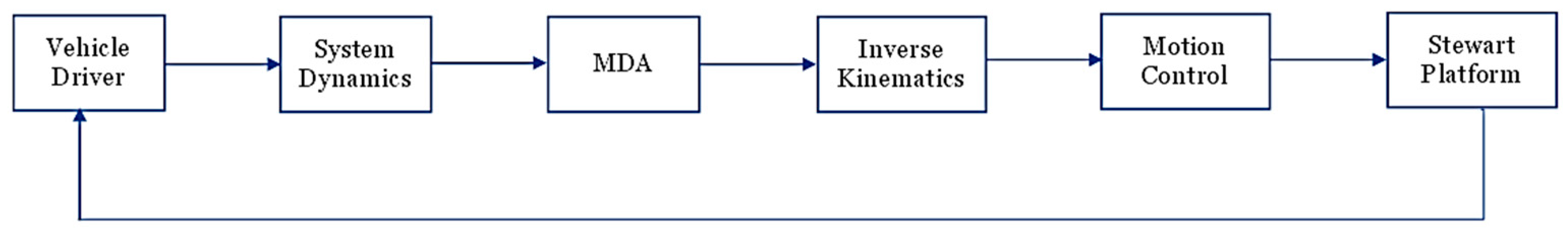
The present study employs an off-road uphill vehicle simulator to implement the suggested algorithm. The simulator utilizes a 6DOF Stewart platform as the motion base. Figure 1 depicts the block diagram of the comprehensive motion simulator system.

The driver operates the vehicle and according to the given driving commands, system dynamics generate the 6DOF motion data. MDA transforms the vehicle motion data according to the restricted platform’s workspace while preserving all the sensory stimuli. The inverse kinematics downstream the motion data as they convert the platform coordinates into the actuator coordinates and determine the required actuator length for all six actuators. Motion control then generates a signal to open/close the actuator’s length to the desired value, which in turn changes the position of the Stewart Platform, and the driver feels the effect like a real vehicle.

The Stewart platform is used as the motion base for the simulator. The Stewart platform is the most popular configuration in parallel manipulators. It offers advantages such as high rigidity, low inertia, and a large load-to-weight ratio. The Stewart platform is the essential essence of motion simulators to provide drivers with a realistic feeling of vehicle driving. In this section, we have described the geometry and inverse kinematics of the platform. The actuators’ dynamics are also presented.

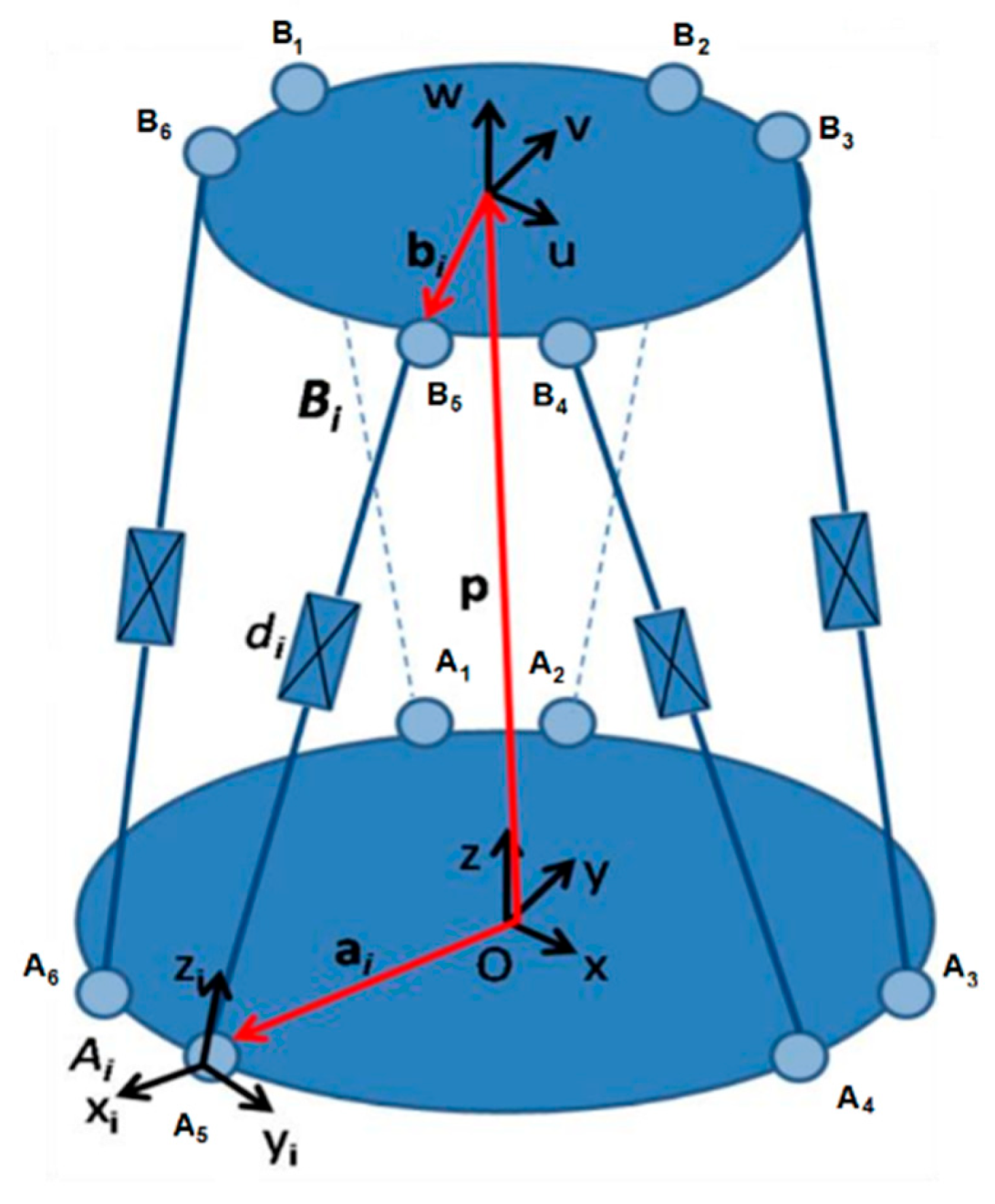
2.1. Stewart Platform Geometry

Using the coordinate system in Figure 2, one frame $A\left(x,y,z\right)$ is connected to the fixed base plate of the platform, and the other frame $B\left(u,v,w\right)$ is associated with the top moving plate of the platform. The mobile platform is connected to the fixed base through six legs (actuators), which are affixed to points $B_i$ and $A_i$ using spherical joints where $i=1,2,\dots ,6$.

The rotation matrix ${}^{A}R_B$ is defined by the angles of yaw $\phi$, roll $\theta$, and pitch $\varphi$ and is given as

$$\begin{array}{l}{}^{A}R_B=\left[\begin{array}{ccc}\mathrm{c}\phi \mathrm{c}\theta & \mathrm{c}\phi \mathrm{s}\theta \mathrm{s}\varphi -\mathrm{c}\varphi \mathrm{s}\phi & \mathrm{c}\phi \mathrm{c}\varphi \mathrm{s}\theta +\mathrm{s}\phi \mathrm{s}\varphi \\ \mathrm{c}\theta \mathrm{s}\phi & \mathrm{c}\phi \mathrm{c}\varphi +\mathrm{s}\phi \mathrm{s}\theta \mathrm{s}\varphi & \mathrm{c}\varphi \mathrm{s}\phi \mathrm{s}\theta -\mathrm{c}\phi \mathrm{s}\varphi \\ -\mathrm{s}\theta & \mathrm{c}\theta \mathrm{s}\varphi & \mathrm{c}\theta \mathrm{c}\varphi \end{array}\right]\\ \mathrm{Where}c=\cos ,s=\sin \end{array}$$

(1)

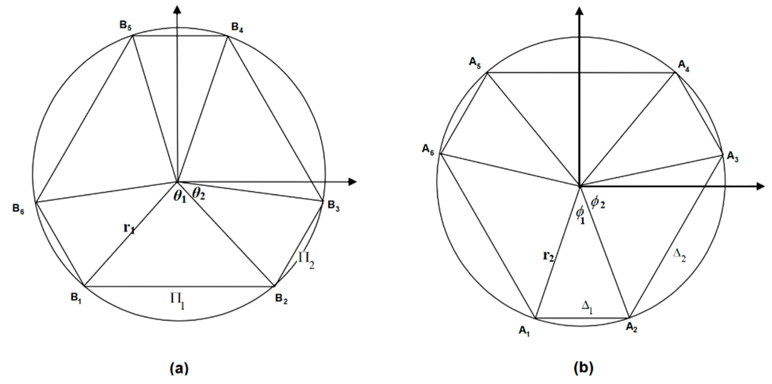
Considering the geometry of the top plate in Figure 3a, the position of each link is the part of the circle intersecting at point $B_1,B_2,\dots ,B_6$. As $u,v$ and $w$ are already defined as the unit orthogonal vectors of the inertial frame of reference, the position vectors of points along $u,v,w$ from the origin, given the value of ${\mathsf{\Pi }}_1$ and ${\mathsf{\Pi }}_2$, are described as

Position vectors along u

$$B_1=-\frac{{\mathsf{\Pi }}_1}{2},B_2=\frac{{\mathsf{\Pi }}_1}{2},B_3=\frac{\left({\mathsf{\Pi }}_1+{\mathsf{\Pi }}_2\right)}{2}$$

$$B_4=\frac{{\mathsf{\Pi }}_2}{2},B_5=-\frac{{\mathsf{\Pi }}_2}{2},B_6=-\frac{\left({\mathsf{\Pi }}_1+{\mathsf{\Pi }}_2\right)}{2}$$

Position vectors along v

$$B_1=-r_1\cos \left(\frac{{\theta }_1}{2}\right),B_2=-r_1\cos \left(\frac{{\theta }_1}{2}\right),B_3=-r_1\sin \left(\frac{\pi }{6}-\frac{{\theta }_2}{2}\right)$$

$$B_4=r_1\cos \left(\frac{{\theta }_2}{2}\right),B_5=r_1\cos \left(\frac{{\theta }_2}{2}\right),B_6=-r_1\sin \left(\frac{\pi }{6}-\frac{{\theta }_2}{2}\right)$$

All the vectors along the $w$ axis are zero for all platform points.

Finally, the positions of the top plate legs joined to the platform are given as

$$\begin{array}{l}{}^{B}b_1={\left[\begin{array}{ccc}-\frac{{\mathsf{\Pi }}_1}{2}& -r_1\cos \left(\frac{{\theta }_1}{2}\right)& 0\end{array}\right]}^T\\ {}^{B}b_2={\left[\begin{array}{ccc}\frac{{\mathsf{\Pi }}_1}{2}& -r_1\cos \left(\frac{{\theta }_1}{2}\right)& 0\end{array}\right]}^T\\ {}^{B}b_3={\left[\begin{array}{ccc}\frac{\left({\mathsf{\Pi }}_1+{\mathsf{\Pi }}_2\right)}{2}& -r_1\sin \left(\frac{\pi }{6}-\frac{{\theta }_2}{2}\right)& 0\end{array}\right]}^T\\ {}^{B}b_4={\left[\begin{array}{ccc}\frac{{\mathsf{\Pi }}_2}{2}& r_1\cos \left(\frac{{\theta }_2}{2}\right)& 0\end{array}\right]}^T\\ {}^{B}b_5={\left[\begin{array}{ccc}-\frac{{\mathsf{\Pi }}_2}{2}& r_1\cos \left(\frac{{\theta }_2}{2}\right)& 0\end{array}\right]}^T\\ {}^{B}b_6={\left[\begin{array}{ccc}-\frac{\left({\mathsf{\Pi }}_1+{\mathsf{\Pi }}_2\right)}{2}& -r_1\sin \left(\frac{\pi }{6}-\frac{{\theta }_2}{2}\right)& 0\end{array}\right]}^T\end{array}$$

(2)

where $r_1=\sqrt{\frac{{\mathsf{\Pi }}_1{}^2+{\mathsf{\Pi }}_2{}^2+2{\mathsf{\Pi }}_1{\mathsf{\Pi }}_2}{3}}$, which is the radius of the circle inscribing the platform’s hexagon.

Now, considering the geometry of the base plate in Figure 3b, the position of each link is the part of the circle inscribing the base hexagon intersection at the points $A_1,A_2,\dots ,A_6$.

So, position vectors of base points along $x,y,z$ from the origin, given the value of ${\mathsf{\Delta }}_1$ and ${\mathsf{\Delta }}_2$, are described as

Position vectors along x

$$A_1=-\frac{{\mathsf{\Delta }}_1}{2},A_2=\frac{{\mathsf{\Delta }}_1}{2},A_3=\frac{\left({\mathsf{\Delta }}_1+{\mathsf{\Delta }}_2\right)}{2}$$

$$A_4=\frac{{\mathsf{\Delta }}_2}{2},A_5=-\frac{{\mathsf{\Delta }}_2}{2},A_6=-\frac{\left({\mathsf{\Delta }}_1+{\mathsf{\Delta }}_2\right)}{2}$$

Position vectors along y

$$A_1=-r_2\cos \left(\frac{{\varphi }_1}{2}\right),A_2=-r_2\cos \left(\frac{{\varphi }_1}{2}\right),A_3=-r_2\sin \left(\frac{\pi }{6}-\frac{{\varphi }_2}{2}\right)$$

$$A_4=r_2\cos \left(\frac{{\varphi }_2}{2}\right),A_5=r_2\cos \left(\frac{{\varphi }_2}{2}\right),A_6=-r_2\sin \left(\frac{\pi }{6}-\frac{{\varphi }_2}{2}\right)$$

All the vectors along the $z$ axis are zero for all platform points.

Finally, the positions of the base plate legs joined to the platform are given as

$$\begin{array}{l}{}^{A}a_1={\left[\begin{array}{ccc}-\frac{{\mathsf{\Delta }}_1}{2}& -r_2\cos \left(\frac{{\varphi }_1}{2}\right)& 0\end{array}\right]}^T\\ {}^{A}a_2={\left[\begin{array}{ccc}\frac{{\mathsf{\Delta }}_1}{2}& -r_2\cos \left(\frac{{\varphi }_1}{2}\right)& 0\end{array}\right]}^T\\ {}^{A}a_3={\left[\begin{array}{ccc}\frac{\left({\mathsf{\Delta }}_1+{\mathsf{\Delta }}_2\right)}{2}& -r_2\sin \left(\frac{\pi }{6}-\frac{{\varphi }_2}{2}\right)& 0\end{array}\right]}^T\\ {}^{A}a_4={\left[\begin{array}{ccc}\frac{{\mathsf{\Delta }}_2}{2}& r_2\cos \left(\frac{{\varphi }_2}{2}\right)& 0\end{array}\right]}^T\\ {}^{A}a_5={\left[\begin{array}{ccc}-\frac{{\mathsf{\Delta }}_2}{2}& r_2\cos \left(\frac{{\varphi }_2}{2}\right)& 0\end{array}\right]}^T\\ {}^{A}a_6={\left[\begin{array}{ccc}-\frac{\left({\mathsf{\Delta }}_1+{\mathsf{\Delta }}_2\right)}{2}& -r_2\sin \left(\frac{\pi }{6}-\frac{{\varphi }_2}{2}\right)& 0\end{array}\right]}^T\end{array}$$

(3)

Let $a_i$ and $b_i$ be vector positions of points $A_i$ and $B_i$ in the given coordinate systems. The mesh equation for the ith actuator of the platform is expressed as follows:

$$\overline{A_i{B}_i}=p+{}^{A}R_B{}^B\mathbf{b}_i-a_i$$

(4)

The length of the ith actuator is determined using

$$d_i=\pm \sqrt{\left[p+{}^{A}R_B{}^B\mathbf{b}_i-a_i\right]\left[p+{}^{A}R_B{}^B\mathbf{b}_i-a_i\right]}$$

(5)

The simplified form is given as

$$\begin{array}{l}{d}_i=\left[p+{}^{A}R_B{}^B\mathbf{b}_i-a_i\right]\\ =\left[\begin{array}{c}x\\ y\\ z\end{array}\right]+\left[\begin{array}{ccc}\mathrm{c}\phi \mathrm{c}\theta & \mathrm{c}\phi \mathrm{s}\theta \mathrm{s}\varphi -\mathrm{c}\varphi \mathrm{s}\phi & \mathrm{c}\phi \mathrm{c}\varphi \mathrm{s}\theta +\mathrm{s}\phi \mathrm{s}\varphi \\ \mathrm{c}\theta \mathrm{s}\phi & \mathrm{c}\phi \mathrm{c}\varphi +\mathrm{s}\phi \mathrm{s}\theta \mathrm{s}\varphi & \mathrm{c}\varphi \mathrm{s}\phi \mathrm{s}\theta -\mathrm{c}\phi \mathrm{s}\varphi \\ -\mathrm{s}\theta & \mathrm{c}\theta \mathrm{s}\varphi & \mathrm{c}\theta \mathrm{c}\varphi \end{array}\right]\left[\begin{array}{c}{b}_{iu}\\ b_{iv}\\ b_{iw}\end{array}\right]-\left[\begin{array}{c}{a}_{ix}\\ a_{iy}\\ a_{iz}\end{array}\right]\\ =\left[\begin{array}{c}x+b_{iu}\mathrm{c}\phi \mathrm{c}\theta +b_{iv}\left(\mathrm{c}\phi \mathrm{s}\theta \mathrm{s}\varphi -\mathrm{c}\varphi \mathrm{s}\phi \right)+b_{iw}\left(\mathrm{c}\phi \mathrm{c}\varphi \mathrm{s}\theta +\mathrm{s}\phi \mathrm{s}\varphi \right)-a_{ix}\\ y+b_{iu}\mathrm{c}\theta \mathrm{s}\phi +b_{iv}\left(\mathrm{c}\phi \mathrm{c}\varphi +\mathrm{s}\phi \mathrm{s}\theta \mathrm{s}\varphi \right)+b_{iw}\left(\mathrm{c}\varphi \mathrm{s}\phi \mathrm{s}\theta -\mathrm{c}\phi \mathrm{s}\varphi \right)-a_{iy}\\ z-b_{iu}\mathrm{s}\theta +b_{iv}\left(\mathrm{c}\theta \mathrm{s}\varphi \right)+b_{iw}\left(\mathrm{c}\theta \mathrm{c}\varphi \right)-a_{iz}\end{array}\right]\end{array}$$

(6)

Therefore, for each given position of the mobile platform, there are two possible solutions for each leg. However, solutions that result in negative leg lengths are physically non-feasible. In instances where the solution assumes a complex number value, the mobile platform’s position is deemed unattainable.

2.2. Inverse Kinematics

In the case of inverse kinematics, we determine the exact leg lengths if we are given the pose (i.e., roll–pitch–yaw) and orientations $\left(x,y,z\right)$. This is achieved by expressing the position of links relative to the position of the end effectors, i.e., local coordinates are determined in terms of global coordinates. For this work, we have used a variant of the Denavit and Hartenberg [45] technique for inverse kinematics.

To find the inverse kinematics equations, consider a given pose and orientation of the platform with translated vector $\left(x,y,z\right)$ and rotational vector ${}^{A}R_B=$ (Rot ($\phi$)*Rot ($\theta$)*Rot ($\varphi$)), provided in Equation (1).

Using the vector theory, the length $d_i$ is determined mathematically [46], as from Figure 2.

$$d_i=T\ast {}^{B}b_i-{}^{A}a_i$$

(7)

$$\left[\begin{array}{c}{d}_{ix}\\ d_{iy}\\ d_{iz}\end{array}\right]=\left[\begin{array}{c}\begin{array}{cccc}\mathrm{c}\phi \mathrm{c}\theta & \mathrm{c}\phi \mathrm{s}\theta \mathrm{s}\varphi -\mathrm{c}\varphi \mathrm{s}\phi & \mathrm{c}\phi \mathrm{c}\varphi \mathrm{s}\theta +\mathrm{s}\phi \mathrm{s}\varphi & x\\ \mathrm{c}\theta \mathrm{s}\phi & \mathrm{c}\phi \mathrm{c}\varphi +\mathrm{s}\phi \mathrm{s}\theta \mathrm{s}\varphi & \mathrm{c}\varphi \mathrm{s}\phi \mathrm{s}\theta -\mathrm{c}\phi \mathrm{s}\varphi & y\\ -\mathrm{s}\theta & \mathrm{c}\theta \mathrm{s}\varphi & \mathrm{c}\theta \mathrm{c}\varphi & z\\ 0& 0& 0& 1\end{array}\end{array}\right]\left[\begin{array}{c}\begin{array}{c}{b}_{iu}\\ b_{iv}\\ b_{iw}\end{array}\\ 1\end{array}\right]-\left[\begin{array}{c}\begin{array}{c}{a}_{ix}\\ a_{iy}\\ a_{iz}\end{array}\\ 1\end{array}\right]$$

(8)

where $d_{ix},d_{iy}$ and $d_{iz}$ are the coordinates of the leg length along the $x,y$ and $z$ axes. The leg length can be determined using the following equation.

$$d_i=\sqrt{{\left(d_{ix}\right)}^2+{\left(d_{iy}\right)}^2+{\left(d_{iz}\right)}^2}$$

(9)

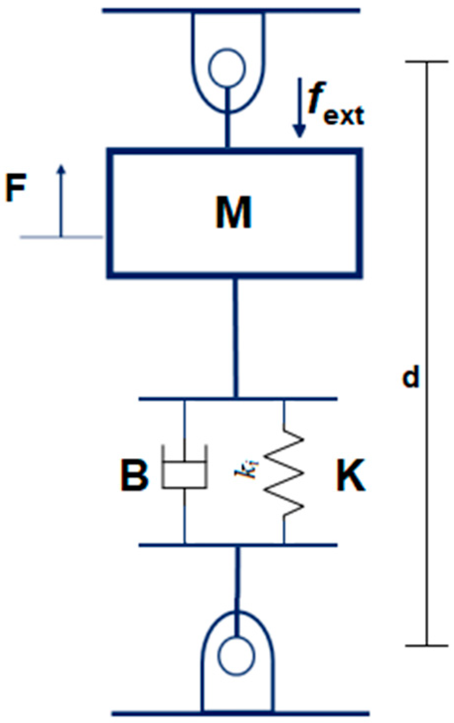
2.3. Actuator’s Dynamics

The Stewart platform is actuated through the utilization of six linear actuators that are affixed to the base plate of the platform and extend to the mounting points located on the top plate. The entire system can be partitioned into six distinct subsystems, with each subsystem composed of a single actuator. It is possible to represent each actuator as a standalone second-order system, as depicted in Figure 4.

The actuator dynamics are modelled as a second-order system and are written as

$$K_i{d}_i\left(t\right)+B_i{\dot{d}}_i\left(t\right)+M_i{\ddot{d}}_i\left(t\right)=F_i\left(t\right)+f_{ext}i=1,2,\dots ,6$$

(10)

where $f_{ext}$ denotes the external force acting on the actuator, $M_i$ the actuator load, $B_i$ the damping coefficient, and $K_i$ the actuator compression coefficient.

3. Fuzzy Adaptive Motion Drive Algorithm Design

MDA design has a key role in motion simulator performance. MDA receives 6DOF motion data from the vehicle dynamics model and generates the required motion sequences within the limits of the Stewart platform. Various types of these algorithms are being used for different simulators, as mentioned in Section 1. We have proposed the IT2 fuzzy adaptive washout algorithm for two reasons. First, an off-road, uphill vehicle simulator has different dynamics as compared to that of a normal driving simulator. Therefore, a constant update is required in filter parameters to avoid falsely generated cues. Second, we have included HVM in the fuzzy controller and subsequently used this information in an adaptive algorithm, which enhances the realism of the simulator. In this section, we discuss the proposed algorithm design.

3.1. Structure of Fuzzy Adaptive MDA

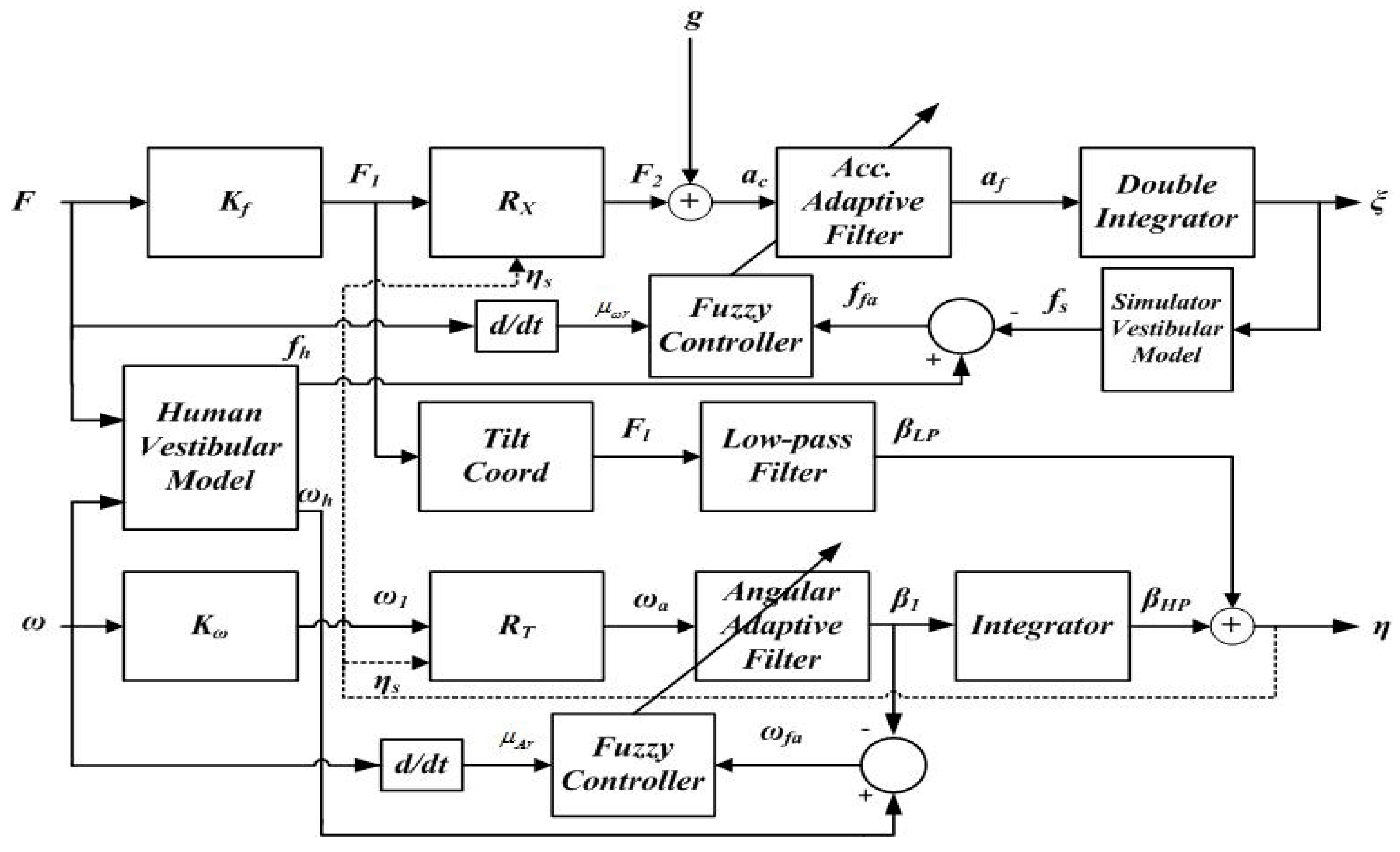
The structure of the proposed fuzzy adaptive MDA seems similar to that of other adaptive washout algorithms. However, it is different in the sense that HVM is used with a fuzzy controller, and adaptive filter coefficients are regularly updated to minimize a loss function. The proposed algorithm is shown in Figure 5.

The algorithm receives body transformed specific forces $F$ and angular rates $\omega$ as input. $K_f$ and $K_{\omega }$ are scaling factors for $F$ and $\omega$, respectively. $R_X$ is a rotation matrix that transforms the angular output vector from the body reference frame to the inertial frame, given in Equation (1), and $R_T$ is a transformation matrix that transforms the angular velocity to Euler angle rates, given as

$$R_T=\left[\begin{array}{ccc}1& \sin \varphi \tan \theta & \cos \varphi \tan \theta \\ 0& \cos \varphi & -\sin \varphi \\ 0& \sin \varphi \sec \theta & \cos \varphi \sec \theta \end{array}\right]$$

(11)

In the first block of the algorithm, specific forces $F$ are scaled based on requirements and simulator limitation, multiplied by the rotational matrix $R_X$, and then passed to the Acceleration Adaptive filter. Forces are also the input of the HVM block, which provides reference sensed specific forces. These forces are then subtracted from measured forces and then passed to the fuzzy controller. The acceleration adaptive filter is composed of an adaptive HPF for $X,Y$ and $Z$ accelerations. It also incorporates fuzzy input and provides translational accelerations. The accelerations are then integrated twice and then the translation position is obtained, i.e., $\xi ={[X,Y,Z]}^T$. In the second block, angular rates are also scaled based on the requirements and multiplied by transformation matrix $R_T$ and then passed to the Angular Adaptive filter. Angular rates are also the input of the HVM block, which provides reference sensed rates. These rates are then subtracted from the measured rates and passed to the fuzzy controller. The angular adaptive filter is composed of an adaptive HPF for the Euler angle rate. It also incorporates fuzzy input and provides filtered rates, which are then integrated to provide a portion of Euler angles. The other portion of Euler angles comes from the LPF of tilt coordination. Tilt coordination is included to incorporate the effect of sustained forces. The two portions combine and provide Euler angles $\eta ={[\varphi ,\theta ,\psi ]}^T$ for rotational motion. The Euler angles are used to calculate $R_X$ and $R_T$ for the next iteration.

3.2. Design of an IT2 Fuzzy Adaptive MDA

The design of the proposed fuzzy adaptive MDA first describes the fuzzy controller design, which is followed by adaptive filter transfer functions and then the selection of adaptive loss functions for parameter update.

3.2.1. Fuzzy Controller Design

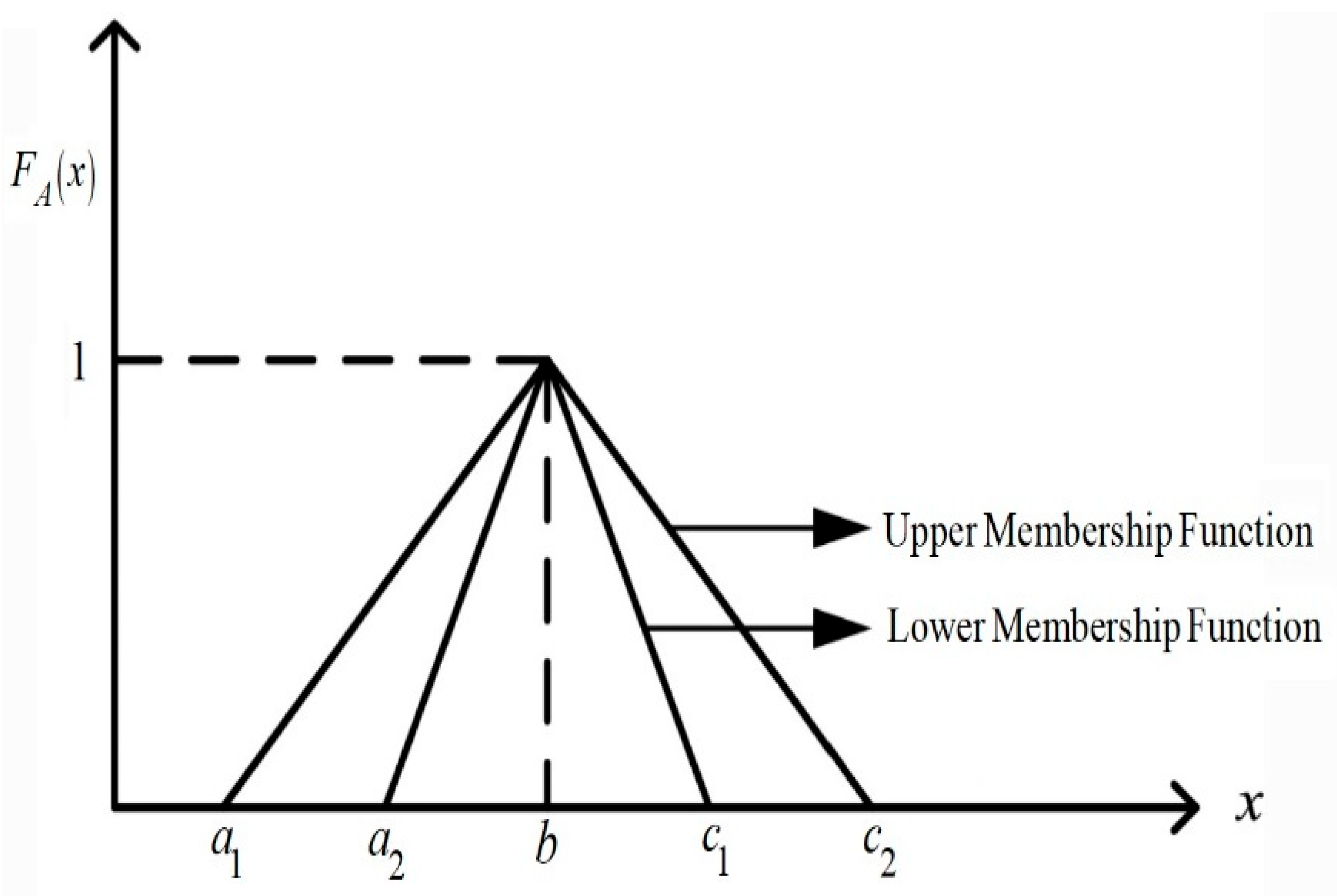
The fuzzy controller is proposed to incorporate HVM to include human perception in the MDA design and to provide a realistic simulator output. For this purpose, an IT2 fuzzy controller is used in this work to produce realistic motion cues while overcoming uncertainty in unknown terrains. A typical IT2 fuzzy membership function is shown in Figure 6, where $F_{\overline{A}}\left(x\right)$ and $F_{\underset{\_}{A}}\left(x\right)$ represent upper and lower membership functions, respectively, and are described below as follows.

$$\begin{array}{l}{F}_{\overline{A}}\left(x\right)=\{\begin{array}{cc}0& x<a_1\\ x-a_1/b-a_1& a_1<x<b\\ 1& x=b\\ c_2-x/c_2-b& b<x<c_2\\ 0& x\ge c_2\end{array}\\ F_{\underset{\_}{A}}\left(x\right)=\{\begin{array}{cc}0& x<a_2\\ x-a_2/b-a_2& a_2<x<b\\ 1& x=b\\ c_2-x/c_2-b& b<x<c_1\\ 0& x\ge c_1\end{array}\end{array}$$

Fuzzy rule base, fuzzification, and defuzzification methods are like type 1 fuzzy systems.

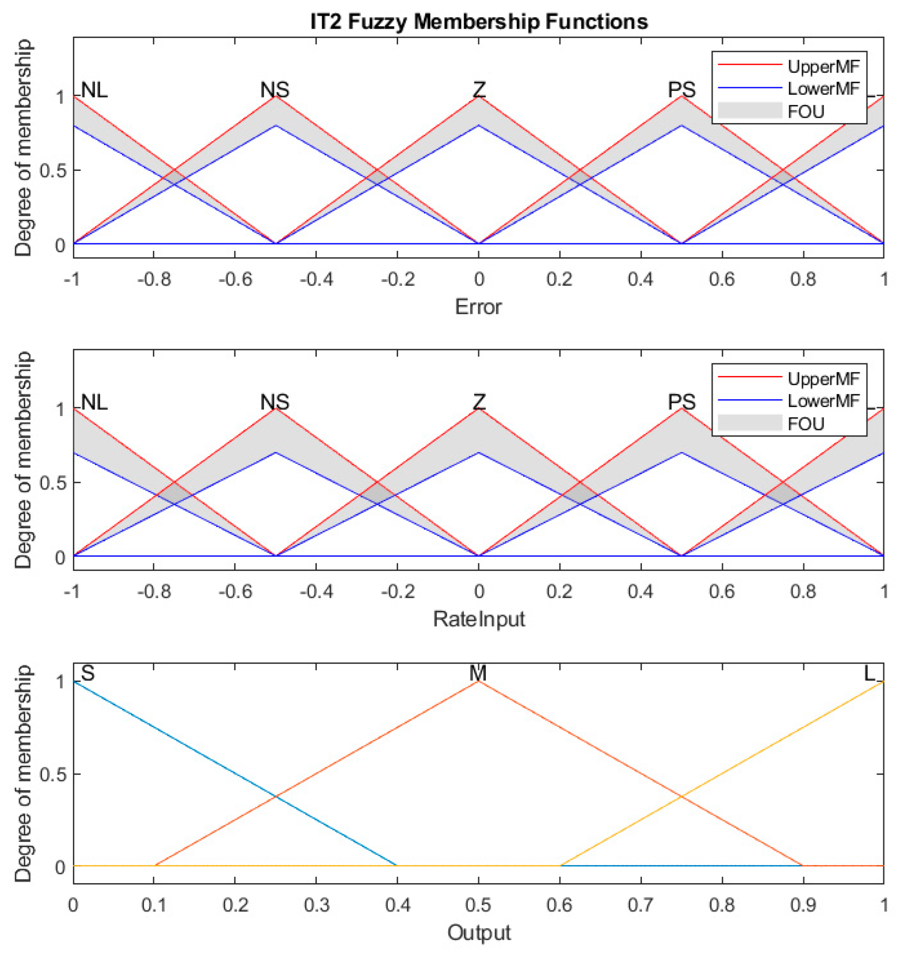
In this work, two fuzzy controllers are used with an acceleration adaptive filter and an angular adaptive filter. The inputs to the first fuzzy controller are specific force rates and an error signal calculated from the difference of reference sensed specific forces and simulator specific forces. The inputs to the second fuzzy controller are angular acceleration and an error signal calculated from the difference of reference sensed rates and measured rates. The inputs are fuzzified into five fuzzy sets, i.e., Negative Large (NL), Negative Small (NS), Zero (Z), Positive Small (PS), and Positive Large (PL). The outputs are fuzzified into three fuzzy sets, i.e., Small (S), Medium (M), and Large (L). Triangular membership functions are selected for input and output variables. Fuzzy rules for the controllers are provided in

Table 3. Fuzzy rules.

	Input Rate
Error	NL	NS	Z	PS	PL
NL	L	L	M	S	S
NS	L	L	M	S	S
Z	L	M	M	M	S
PS	L	M	M	M	S
PL	M	M	M	S	S

. The rule can be explained for the first row as follows:

If the error is NL and input rate is also NL, then output is Large.

If the error is NL and input rate is also NS, then output is Large.

If the error is NL and input rate is also Z, then output is Medium.

If the error is NL and input rate is also PS, then output is Small.

If the error is NL and input rate is also PL, then output is Small.

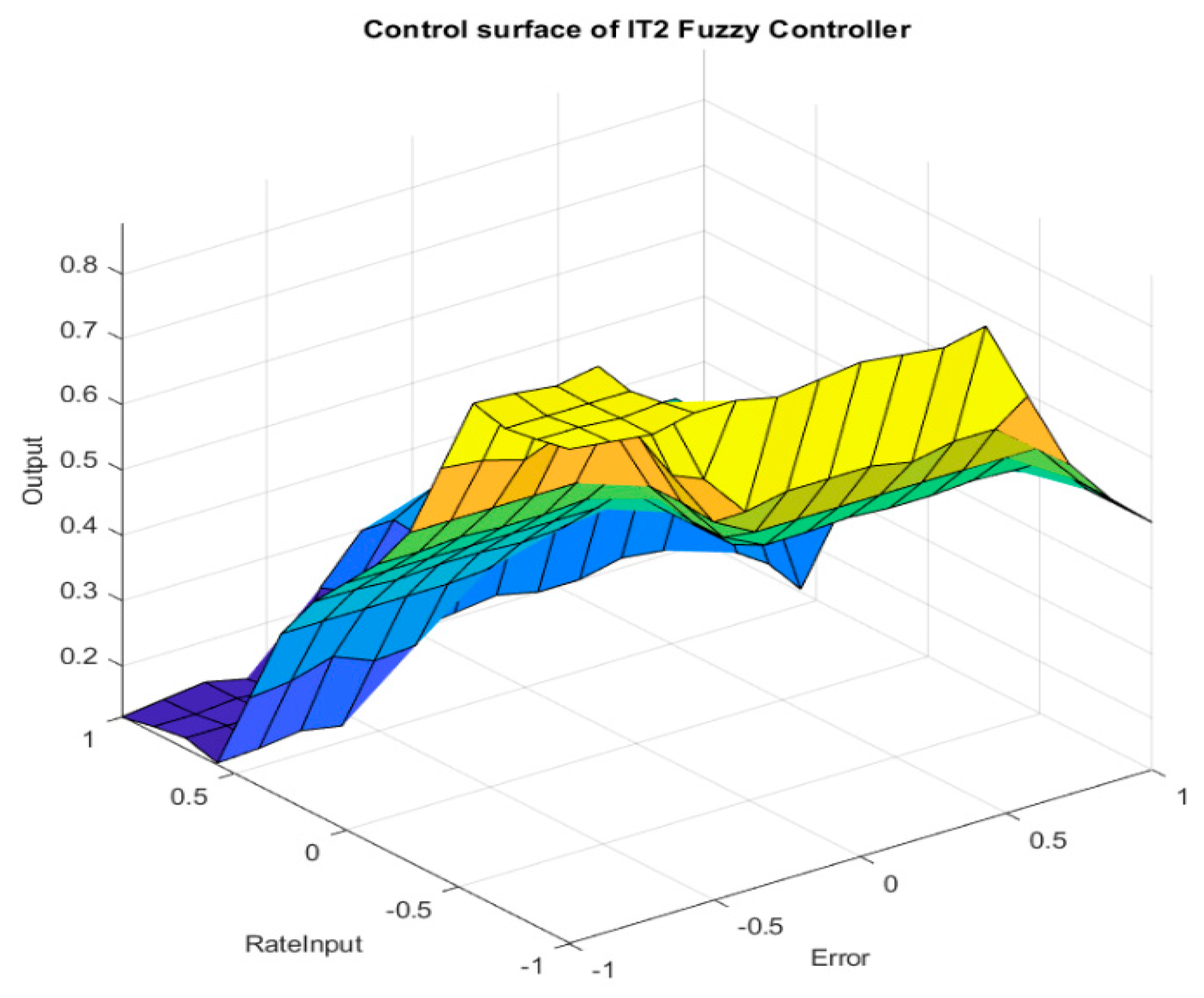
Fuzzy surface plots and membership functions are shown in Figure 7 and Figure 8, respectively. The centroid de-fuzzification method is used to determine the output of the fuzzy controllers. A fuzzy control surface is a stereoscopic three-dimensional map that shows both input and output simultaneously. This facilitates the testing of output for any combination of inputs and output range. For instance, the plot shows that the highest output is less than 0.8.

3.2.2. Adaptive Filter Transfer Functions

The proposed fuzzy adaptive MDA consisted of six HPFs (three for acceleration adaptive filter and angular adaptive filters, respectively) and two LPFs. All HPFs are adaptive in nature, whereas the LPFs are classical LPFs used for tilt coordination.

Acceleration adaptive filters are second-order filters designed for $X,Y$ and $Z$ accelerations. The transfer function of a filter is defined as

$$\frac{a_f{}^{\xi }}{a_c{}^{\xi }}=K_{\xi }\frac{s^2}{s^2+2{\zeta }_{\xi }{\omega }_{1\xi }{w}_{\xi }s+{\omega }_{1\xi }{w}_{\xi }}\mathrm{for} \xi =X,Y,Z$$

(12)

where $K_{\xi }$ is adaptive gain and ${\omega }_{1\xi }$ is fuzzy controller output.

Angular adaptive filters are first-order filters designed for Euler rates. The transfer function of a filter is defined as

$$\frac{{\beta }_{HP}{}^{\eta }}{{\beta }_1{}^{\eta }}=K_{\eta }s\frac{\mathrm{s}}{\mathrm{s}+{\omega }_{2\eta }{w}_{\eta }}\mathrm{for} \mathrm{each} \eta =\theta , \varphi , \psi$$

(13)

where $K_{\eta }$ is adaptive gain and ${\omega }_{2\eta }$ is fuzzy controller output.

The LPFs for tilt coordination are defined as

$$\frac{{\beta }_{LP}{}^{\alpha }}{{\mathrm{F}}_l}=\frac{1}{9.8}\frac{s^2}{s^2+2w_{\alpha }s+w_{\alpha }{}^2}\mathrm{for} \mathrm{each} \alpha =x,y$$

(14)

3.2.3. Adaptive Loss Functions

The adaptive loss functions or cost functions are used to update filter parameters. It is a method for measuring the filter’s performance and modifying its behavior accordingly. Similar to a feedback mechanism, it aids the filter in adapting and enhancing its performance over time. The loss functions are summation of products of weights and various factors that help to evade false motion in the Stewart platform and return it to the base position in case of sustained motions. It also ensures the simulator’s operation within defined simulator boundaries.

Three adaptive loss functions are formulated for (i) X/pitch (CP), (ii) roll/Y (CR), and (iii) yaw/Z (CY). The adaptive loss functions are determined as

$$\begin{array}{l}{C}_P=\frac{1}{2}\left[W_{p1}{\left(\dot{x}\right)}^2+W_{p2}{\left(x\right)}^2+W_{p3}{\left({\dot{\theta }}_0\right)}^2+W_{p4}{\left({\theta }_0\right)}^2+W_{p5}{\left(K_{x1}-K_{x0}\right)}^2+W_{p6}{\left(K_{\theta 1}-K_{\theta 0}\right)}^2\right]\\ C_R=\frac{1}{2}\left[W_{r1}{\left(\dot{y}\right)}^2+W_{r2}{\left(y\right)}^2+W_{r3}{\left({\dot{\varphi }}_0\right)}^2+W_{r4}{\left({\varphi }_0\right)}^2+W_{r5}{\left(K_{y1}-K_{y0}\right)}^2+W_{r6}{\left(K_{\varphi 1}-K_{\varphi 0}\right)}^2\right]\\ C_Y=\frac{1}{2}\left[W_{y1}{\left(\dot{z}\right)}^2+W_{y2}{\left(z\right)}^2+W_{y3}{\left({\dot{\psi }}_0\right)}^2+W_{y4}{\left({\psi }_0\right)}^2+W_{y5}{\left(K_{z1}-K_{z0}\right)}^2+W_{y6}{\left(K_{\psi 1}-K_{\psi 0}\right)}^2\right]\end{array}$$

(15)

where $W_{}$ denotes weight values used in each function. $W_1$ and $W_2$ are responsible for minimization of position error. $W_3$ and $W_4$ are responsible for minimization of motion cues error. $W_5$ and $W_6$ are responsible for maintaining the parameters’ values within limits.

The gradient descent method is employed for minimization of the proposed functions. The adaptive parameters are updated for each sample n with the following formula:

(i) X

$$\begin{array}{l}\mathsf{\Delta }{K}_x(n)=-{\lambda }_x\frac{\partial C_P}{\partial K_x}\\ K_x\left(n\right)=K_x\left(n-1\right)+\mathsf{\Delta }{K}_x\left(n\right)+\mathsf{\gamma }\left[K_x\left(n-1\right)-K_x\left(n-2\right)\right]\end{array}$$

(16)

(ii) Y

$$\begin{array}{l}\mathsf{\Delta }{K}_y(n)=-{\lambda }_y\frac{\partial C_R}{\partial K_y}\\ K_y\left(n\right)=K_y\left(n-1\right)+\mathsf{\Delta }{K}_y\left(n\right)+\mathsf{\gamma }\left[K_y\left(n-1\right)-K_y\left(n-2\right)\right]\end{array}$$

(17)

(iii) Z

$$\begin{array}{l}\mathsf{\Delta }{K}_z(n)=-{\lambda }_z\frac{\partial C_Y}{\partial K_z}\\ K_z\left(n\right)=K_z\left(n-1\right)+\mathsf{\Delta }{K}_z\left(n\right)+\mathsf{\gamma }\left[K_z\left(n-1\right)-K_z\left(n-2\right)\right]\end{array}$$

(18)

(iv) Pitch

$$\begin{array}{l}\mathsf{\Delta }{K}_{\theta }(n)=-{\lambda }_{\theta }\frac{\partial C_P}{\partial K_{\theta }}\\ K_{\theta }\left(n\right)=K_{\theta }\left(n-1\right)+\mathsf{\Delta }{K}_{\theta }\left(n\right)+\mathsf{\gamma }\left[K_{\theta }\left(n-1\right)-K_{\theta }\left(n-2\right)\right]\end{array}$$

(19)

(v) Roll

$$\begin{array}{l}\mathsf{\Delta }{K}_{\varphi }(n)=-{\lambda }_{\varphi }\frac{\partial C_R}{\partial K_{\varphi }}\\ K_{\varphi }\left(n\right)=K_{\varphi }\left(n-1\right)+\mathsf{\Delta }{K}_{\varphi }\left(n\right)+\mathsf{\gamma }\left[K_{\varphi }\left(n-1\right)-K_{\varphi }\left(n-2\right)\right]\end{array}$$

(20)

(vi) Yaw

$$\begin{array}{l}\mathsf{\Delta }{K}_{\psi }(n)=-{\lambda }_{\psi }\frac{\partial C_Y}{\partial K_{\psi }}\\ K_{\psi }\left(n\right)=K_{\psi }\left(n-1\right)+\mathsf{\Delta }{K}_{\psi }\left(n\right)+\mathsf{\gamma }\left[K_{\psi }\left(n-1\right)-K_{\psi }\left(n-2\right)\right]\end{array}$$

(21)

where ${\lambda }_{x,y,\theta ,\varphi ,\psi }\in \left(0,1\right)$ shows learning factor and $\mathsf{\gamma }\in \left(0,1\right)$ shows momentum factor.

4. Results and Discussions

In this section, the performance evaluation of the proposed algorithm on an off-road, uphill vehicle simulator is presented. The motion specifications of the Stewart platform are given in

Table 4. Stewart platform specifications.

Degree of Freedom	Displacement	Velocity	Acceleration
Pitch	±15 deg	±30 deg/s	±150 deg/s2
Roll	±15 deg	±28 deg/s	±150 deg/s2
Yaw	±18 deg	±35 deg/s	±150 deg/s2
Heave	±0.15 m	±0.35 m/s	+0.6 G
Surge	±0.19 m	±0.50 m/s	±0.6 G
Sway	±0.20 m	±0.50 m/s	±0.6 G

. The specifications also indicate the motion’s limitations. The work also has another limitation, which is that the proposed algorithm is designed for a 6-DOF motion platform and is therefore inapplicable to lesser DOF motion platforms. There are no specific criteria for the selection of gains and filters’ weights. After a few iterations, the selected parameters for the proposed fuzzy adaptive MDA are given in

Table 5. Adaptive washout filter parameters.

Parameters	Value	Parameters	Value
Kf	0.33	Learning rate $\lambda$	0.13
Kω	0.5	Momentum factor $\mathsf{\gamma }$	0.20
$w_X$	4	$W_1$ for pitch, roll, yaw	0.4
$w_Y$	4	$W_2$ for pitch, roll, yaw	0.4
$w_Z$	4.3	$W_3$ for pitch, roll	0.45
${\zeta }_X$	0.9	$W_4$ for pitch, roll	0.45
${\zeta }_Y$	0.9	$W_5$ for pitch, roll, yaw	0.4
${\zeta }_Z$	0.5	$W_6$ for pitch, roll	0.45
$w_{\theta }$	3	$W_3$ for yaw	0.33
$w_{\varphi }$	3	$W_4$ for yaw	0.33
$w_{\psi }$	2.5	$W_6$ for yaw	0.33

.

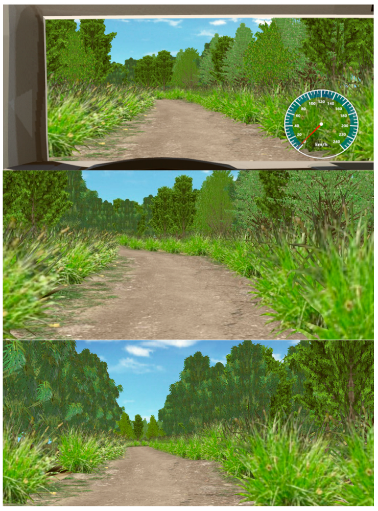
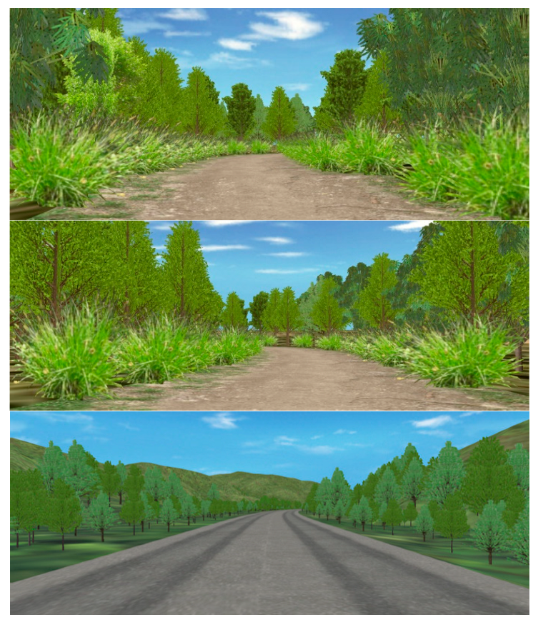
The Truck was selected to drive on mountain tracks developed in UC-Win/Road. Some random screenshots of the simulated environment are shown in Figure 9. The experiment was performed with haphazard driving, especially on the yaw axis, rather than smooth driving, to check the performance of the proposed algorithm. The rotational angles were measured using the Attitude Heading Reference Sensor (AHRS) mounted on the Stewart platform, whereas forward kinematics were used to find translation motion values. In the experiment, the proposed algorithm on an off-road, uphill vehicle simulator provided realistic motion cues. Although the performance of a driving simulator can only be evaluated by driving it based on the quality of the ride the driver experiences, for evaluation, we have compared our results with the classical algorithm. The approach has also been adopted by other researchers who have developed MDA and washout filters [33,34,39,47,48]. For this purpose, the experimental motion data were recorded to compare the proposed algorithm’s response with classical washout filters. All the results have two components. In the first section, the input to the algorithm is displayed, while in the second section, the responses of the proposed MDA and the classical MDA are displayed. The x-axis depicts the number of samples. There are 15 samples per second, so the average response time is approximately 5 min and 30 s.

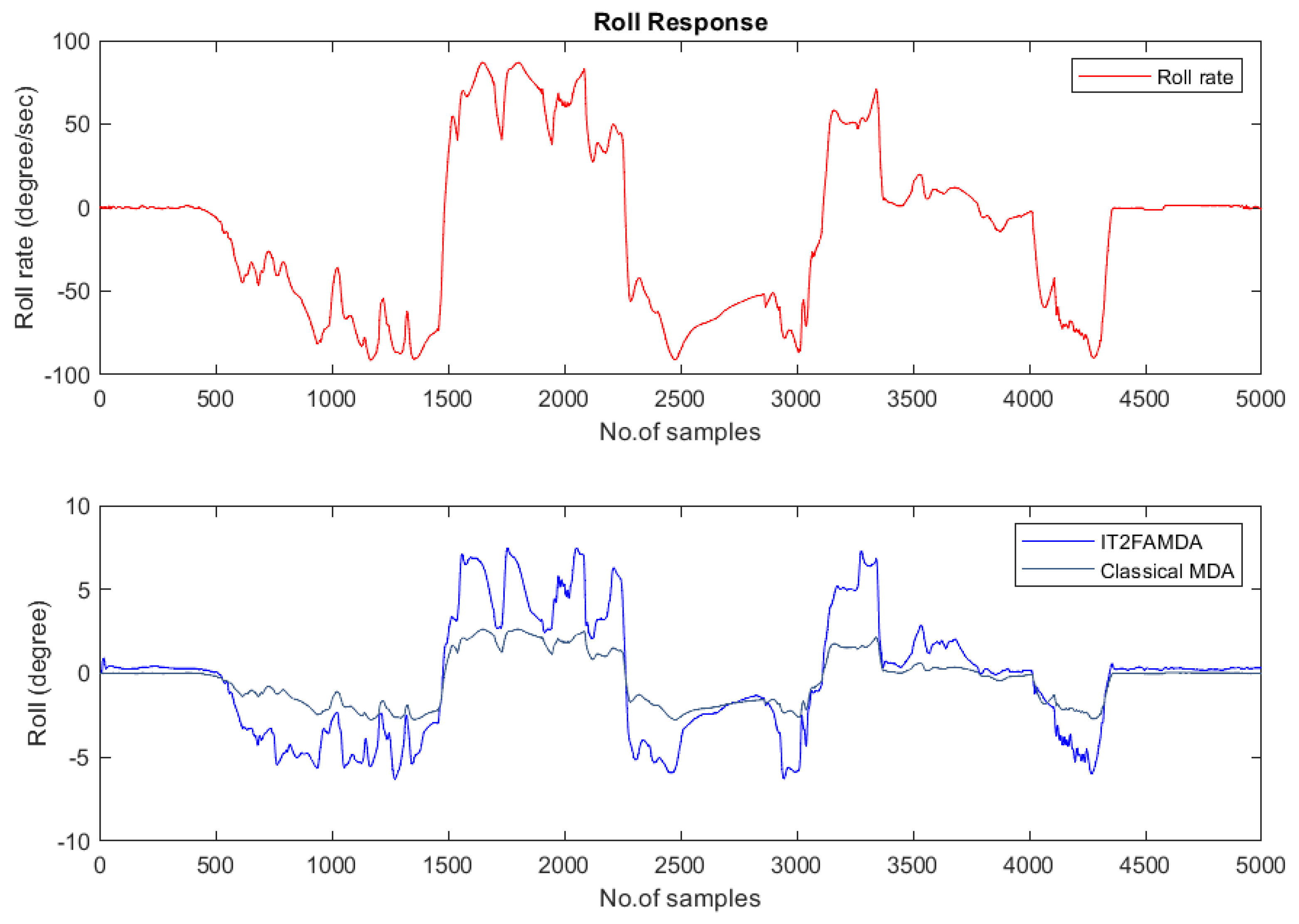
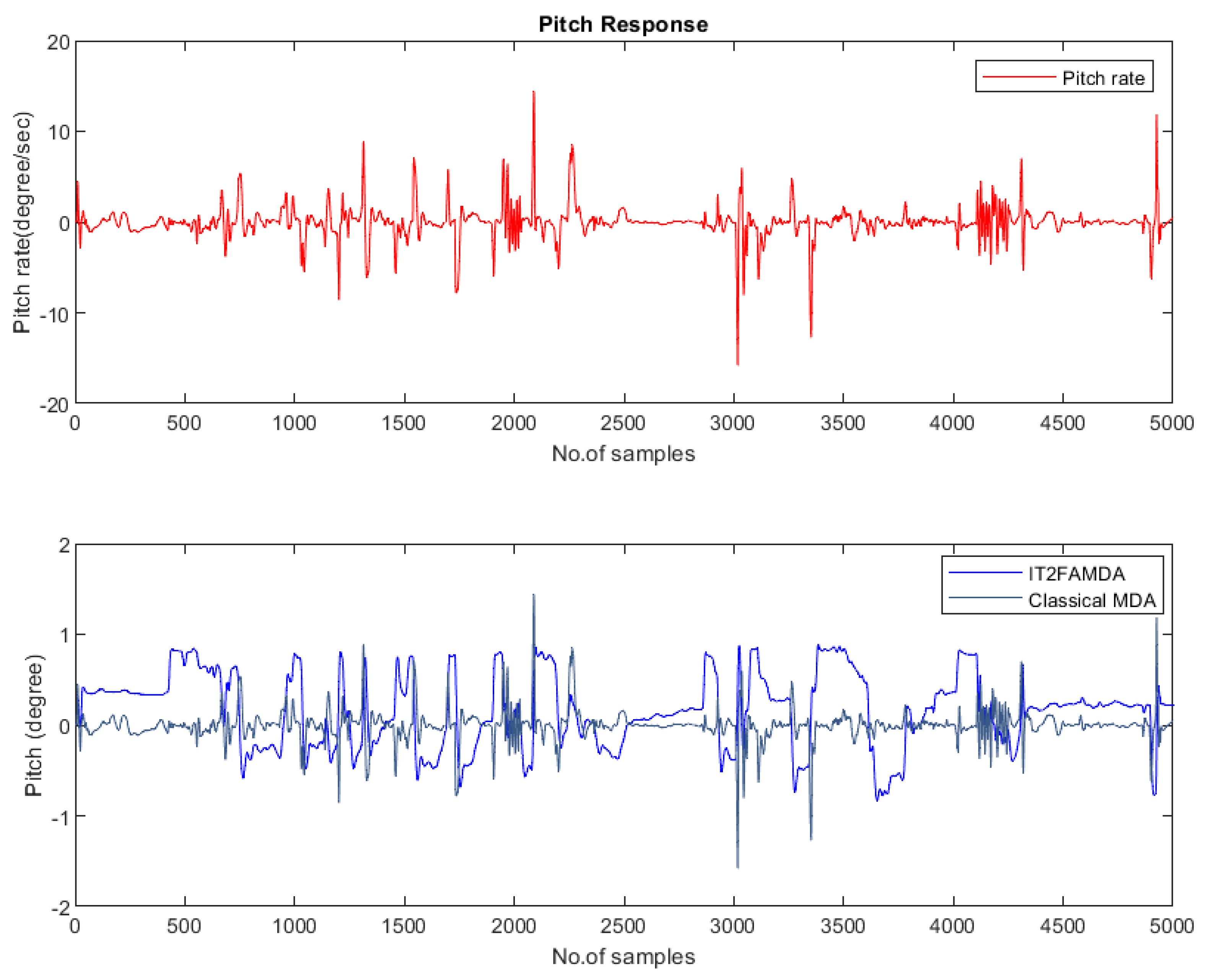
The roll and pitch responses of the proposed MDA are shown in Figure 10 and Figure 11, respectively. Roll and pitch motion cues are not as significant for urban ground vehicle simulators but they are very important in off-road uphill simulators, as tracks are not uniform and Roll and Pitch reflect the road and driving conditions. A good washout filter should let the driver experience variable road and driving conditions. For these responses, we have used rough terrains. The result in Figure 10 shows that the proposed algorithm offers true rolling sensation as compared to the classical algorithm. It is also important to note that the proposed algorithm has allowed the driver to truly experience the abrupt change that is caused by ditches while still ensuring the driver’s safety. This is an important achievement for the algorithm. There is evidence of it in sample numbers 1500, 2275, 3100, and 4300 respectively. On the contrary, the classical algorithm has suppressed the response. In the case of the largest unexpected change, which occurred at sample number 1500, the proposed algorithm translated the response to the driver in a seamless manner. The response of the pitch is shown to be more smooth in Figure 11 when compared to the classical MDA. Despite this, there are not many jarring shifts discernible in the response of classical MDA. For example, the driver will experience jerks when using the classical MDA at samples 1230, 2150, 3020, 3400, and 4900, respectively. However, the proposed algorithm is able to handle these jerks in a smooth manner and permit the driver to experience them while remaining within acceptable safety parameters.

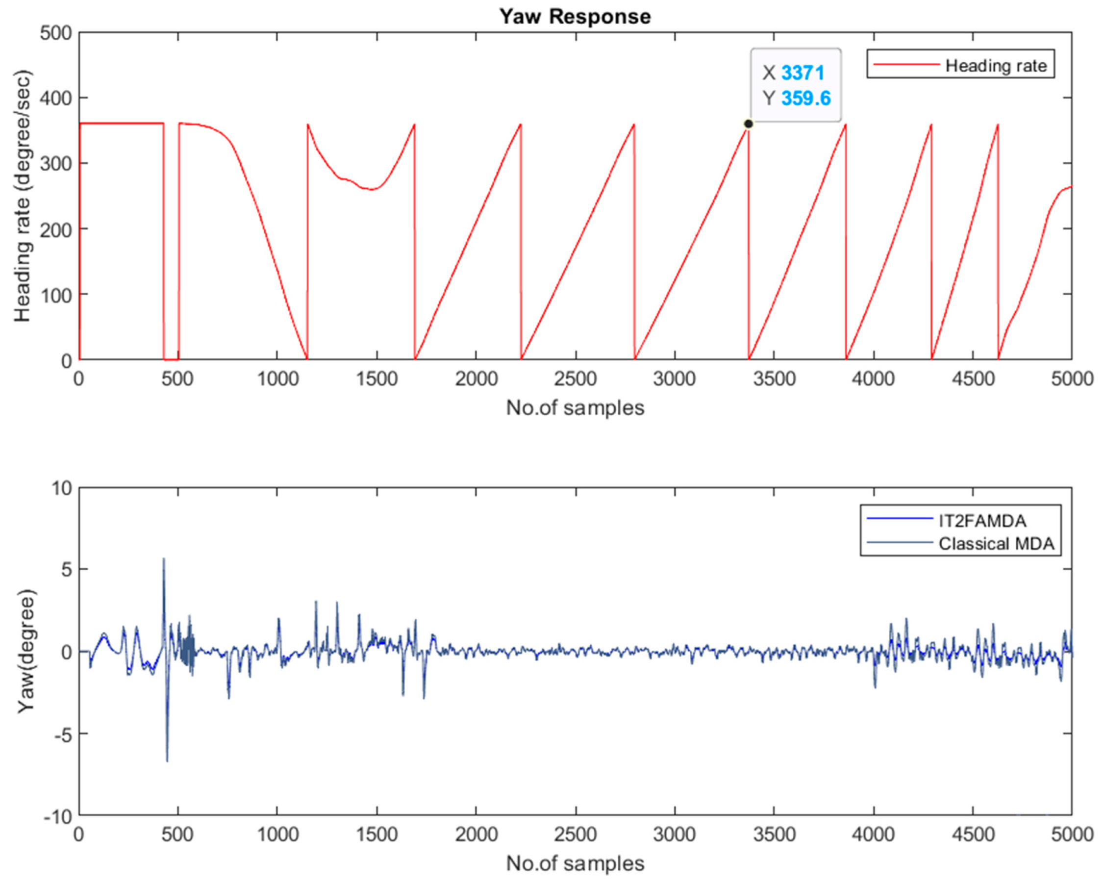
The yaw motion response is illustrated in Figure 12. For this motion, the vehicle was initially constantly turned to the right, then to the left for 250 samples, and then back to the right for the remaining 3300 samples. Initially, the proposed MDA and classical MDA demonstrated comparable performance, but false cues can be observed in the response of the classical MDA after continuously varying heading rate. Figure 12 also demonstrates that the yaw response is very smooth despite the constantly changing heading rate.

In addition to the drivers’ testimonials trained on the proposed simulator, all the provided responses clearly indicate that the proposed IT2 fuzzy-based adaptive motion drive algorithm provides better performance as compared to the classical MDA on mountain tracks. The proposed MDA has avoided false cues that are present in classical MDA responses.

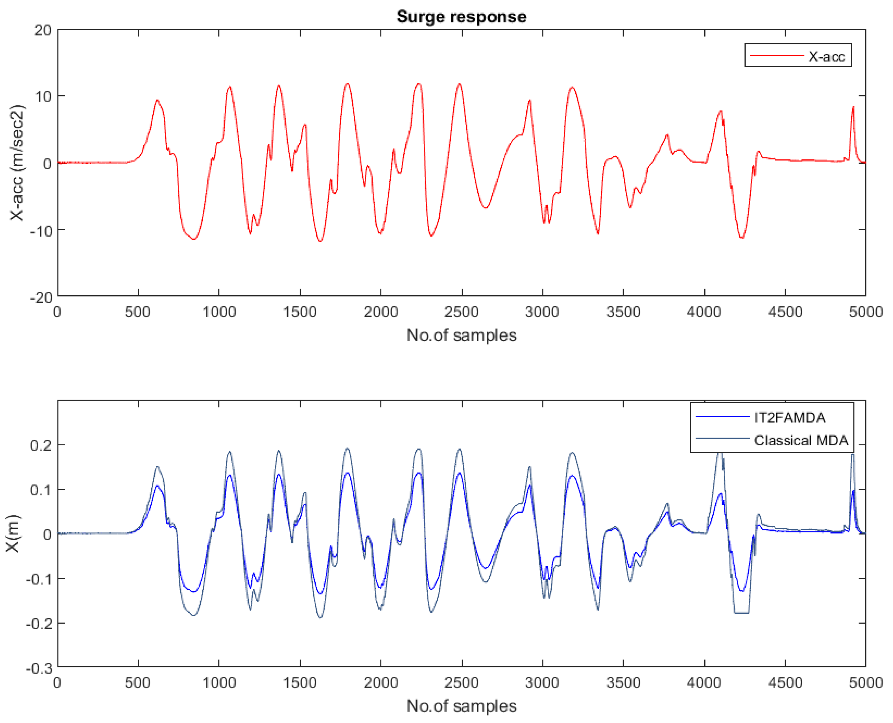
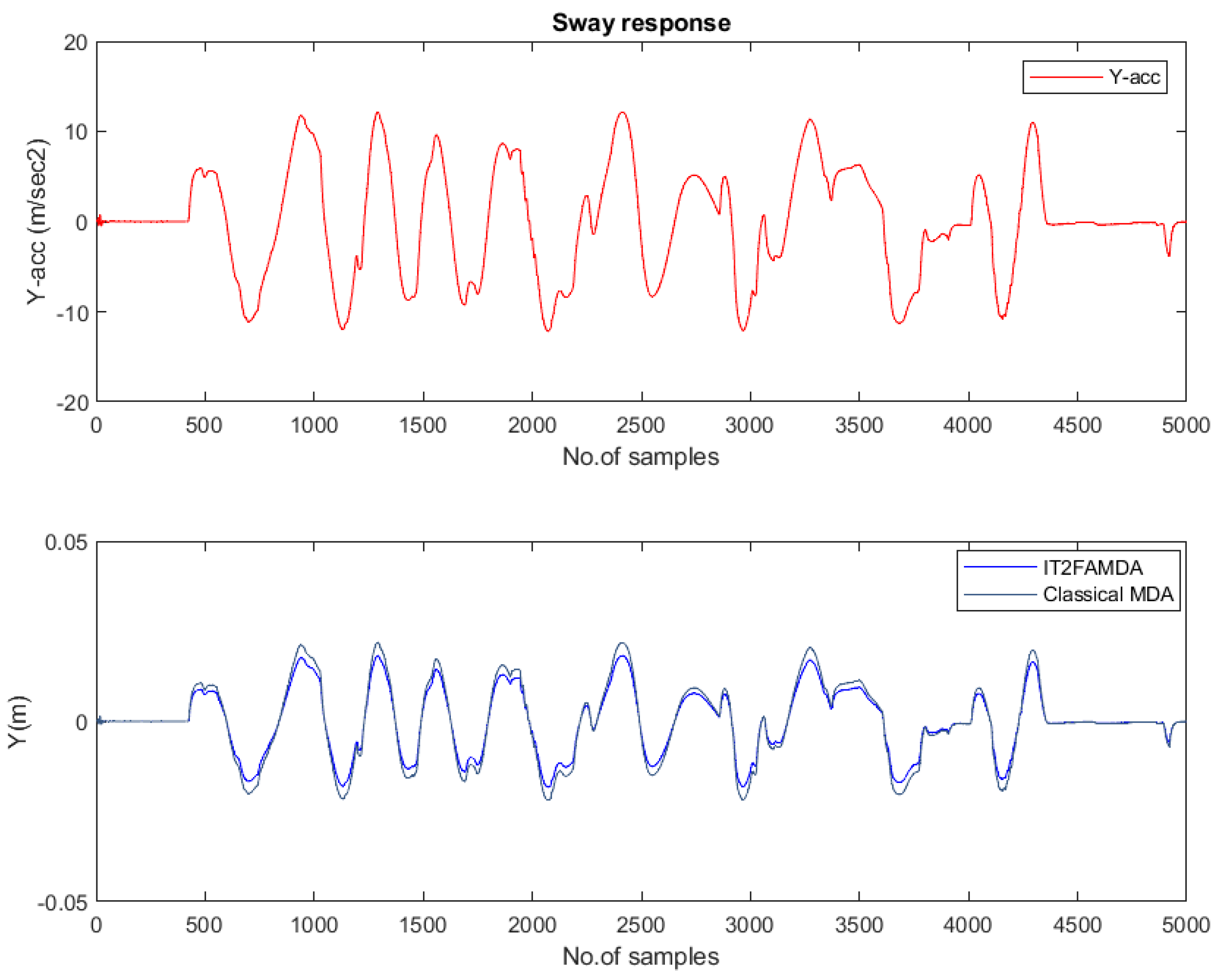
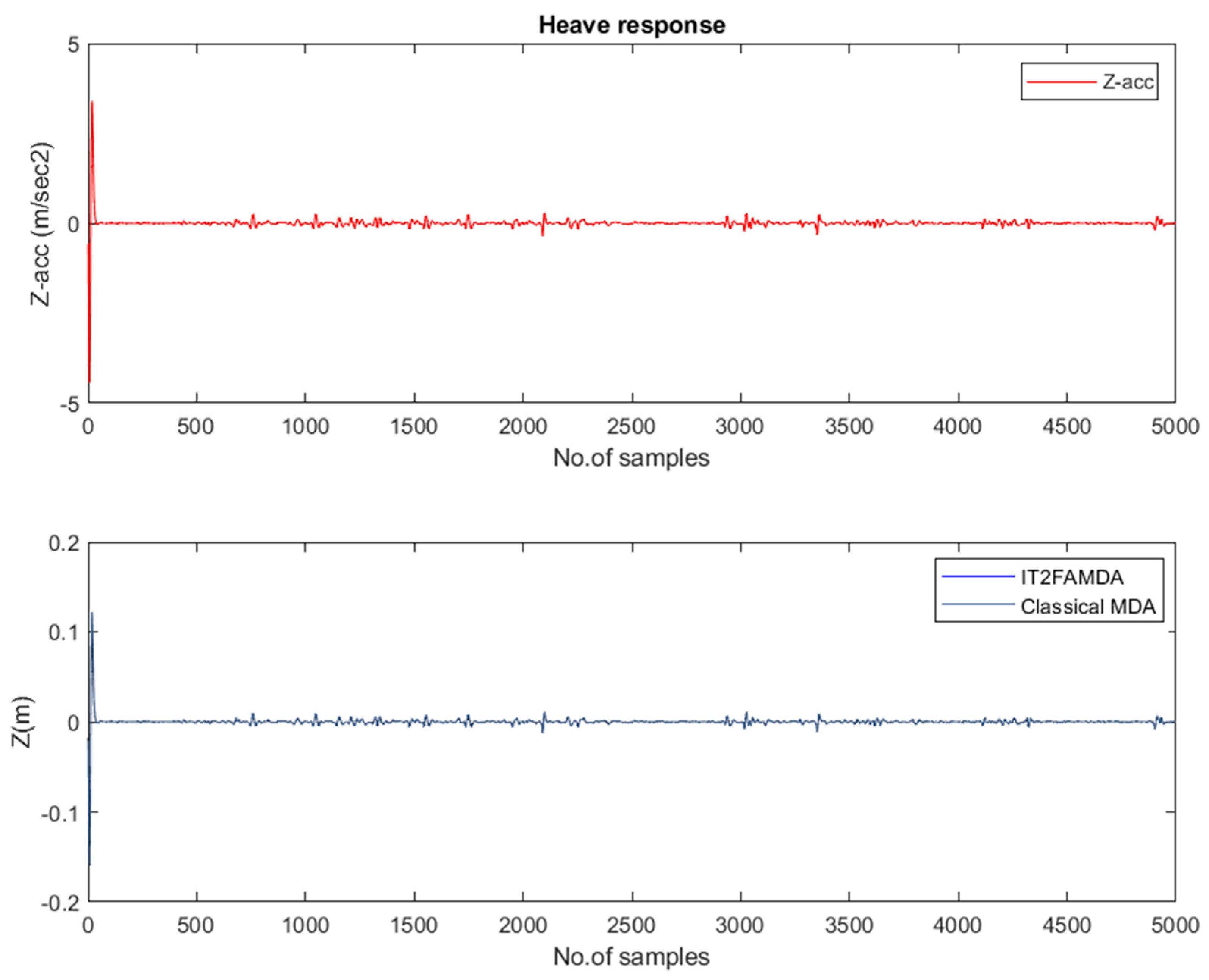
Responses for translation motions are provided in Figure 13, Figure 14 and Figure 15. When it comes to ground vehicle simulators, only the surge motion is more important than the sway and heave movements. This is because the vehicle can only move in one direction, forward. For this response, the driver was asked to move the car forward, then slowly apply the brakes, then move the car forward, and do this over and over again. The positive accelration shows the movement in the forward direction, whereas the negative acceleration shows the braking phenomena. Figure 13 shows that when the brake is used, the proposed MDA was able to bring the Stewart platform back to the neutral position. Moreover, the Stewart platform never reached the maximum allowable surge movement. In this experiment, on the other hand, classical MDA caused the Stewart platform to reach the surge movement limit three times and potentially decreased the allowable limits for other DOF motions. Figure 14 shows the similar sway motion response for both algorithms except at peaks, where the proposed algorithm response is different because of continuously updating adaptive gains. Figure 15 shows an almost similar response for both filters because a simple HP filter was used for the heave channel, as the heave channel has no significance in ground vehicle simulators.

In summary, it is observed in the test drive that the proposed algorithm has proved more efficient than classical MDA for the ground vehicle simulator. The usage of the IT2 fuzzy-based adaptive washout filter resulted in a smooth drive and avoided any false motion cues. Furthermore, due to continuous updates of adaptive parameters, the motion platform remained within the allowable motion envelope.

5. Conclusions

This article introduces a novel IT2 fuzzy adaptive motion drive algorithm for high-fidelity motion cuing and realistic simulation of the ground vehicle simulator in mountainous regions. This paper provides an overview of the current state of the art regarding driving simulators and motion drive algorithms. The geometry, kinematics, and actuator dynamic model of the Stewart platform are discussed in depth. The design of the proposed algorithm is presented in detail. The proposed algorithm response is compared to the classical washout algorithm response on an off-road uphill vehicle simulator. In addition to the testimonials of drivers trained on the proposed simulator, simulation results demonstrate that the proposed IT2 fuzzy-based adaptive motion drive algorithm provides superior performance on mountain tracks compared to the classical washout algorithm. The pitch and roll responses demonstrate that the proposed algorithm has enabled the driver to experience the abrupt changes caused by ditches while maintaining the driver’s safety. The classical algorithm, on the other hand, restricted the roll response and provided a jerky pitch response. The surge response demonstrated that the proposed MDA handled the acceleration and deceleration of the vehicle very effectively. In addition, the Stewart platform never reached the permitted maximum surge motion. Classical MDA, on the other hand, caused the Stewart platform to reach the surge movement limit three times and possibly lowered the allowable limits for other DOF motions. Numerous practical implications and potential applications exist for the proposed simulator in a variety of industries. The automotive industry, particularly manufacturers and suppliers of off-road vehicles, could greatly benefit from the findings of this study. It could aid in vehicle development and testing, improving off-road performance, and enhancing off-road driving safety features. For training purposes, military organizations and defense contractors may find the simulator useful. It could aid in simulating difficult terrains and scenarios encountered during military operations, allowing soldiers and personnel to practice off-road driving in a safe, controlled environment. Future work could include data collection and analysis for performance evaluation, machine learning techniques for adaptive simulation, or integration with other emerging technologies like AI for intelligent driver assistance systems.