Article

Single-Image Dehazing Based on Improved Bright Channel Prior and Dark Channel Prior

1
College of Computer and Information Science, Southwest University, Chongqing 400715, China
2
College of Big Data and Intelligent Engineering, Chongqing College of International Business and Economics, Chongqing 401520, China
3
College of Big Data and Artificial Intelligence, Chizhou University, Chizhou 247000, China
4
College of Electronic and Information Engineering, Southwest University, Chongqing 400715, China
*
Author to whom correspondence should be addressed.
Electronics 2023, 12(2), 299; https://doi.org/10.3390/electronics12020299
Submission received: 29 November 2022 / Revised: 26 December 2022 / Accepted: 29 December 2022 / Published: 6 January 2023
(This article belongs to the Special Issue Artificial Intelligence Technologies and Applications)

Abstract

:
Single-image dehazing plays a significant preprocessing role in machine vision tasks. As the dark-channel-prior method will fail in the sky region of the image, resulting in inaccurately estimated parameters, and given the failure of many methods to address a large band of haze, we propose a simple yet effective method for single-image dehazing based on an improved bright prior and dark channel prior. First, we use the Otsu method by particle swarm optimization to divide the hazy image into sky regions and non-sky regions. Then, we use the improved bright channel prior and dark channel prior to estimate the parameters in the physical model. Second, we propose a weighted fusion function to efficiently fuse the parameters estimated by two priors. Finally, the clear image is restored through the physical model. Experiments illustrate that our method can solve the problem of the invalidation of the dark channel prior in the sky region well and achieve high-quality image restoration, especially for images with limited haze.

1. Introduction

Complex weather, such as haze, will decrease the visibility of the landscape and affect the image quality. For example, there will be missing colors, low saturation and blurred texture details, which will lead to a decrease in the accuracy of vision system tasks.
Image dehazing methods can be divided into: image enhancement-based, prior-based and deep learning-based methods. Enhanced-based dehazing methods such as Retinex [1], histogram equalization [2] and wavelet transform [3] do not depend on the physical model and improve image quality by increasing contrast and saturation. However, this kind of method does not have a good dehazing effect and does not realize real dehazing physically. Prior-based image dehazing methods generally estimate the parameters (transmission map and atmospheric light) of the atmospheric scattering model (ASM) [4,5,6] and recover sharp images. For example, He et al. [7] proposed the dark channel prior (DCP) to estimate the transmission map. DCP is a well-known prior, which assumes that low-intensity values of at least one color channel in a haze-free image are close to zero [8]. Meng [9] proposed boundary constraints and regularization (BCCR), which uses guided filtering and bilateral filtering to replace time-consuming soft matting to improve computational efficiency. Berman [10] discovered a haze line prior (NonLocal), that is, the color value distribution of the image will change from clusters to lines due to the existence of haze, and used this distribution rule to make a preliminary estimate of the transmission map. Some scholars have also proposed some methods combining total variation and DCP to estimate the parameters [11,12,13]. These prior-based methods, although somewhat successful, rely on estimates of parameters but are prone to problems such as distortion.
Recently, learning-based methods have received more attention. Scholars have begun to explore the use of convolutional neural networks (CNN) for image dehazing. Early image dehazing methods focused on using the estimated transmission map to restore the hazy images. For example, Li [14] proposed an AOD-Net, which reformulated ASM and put a transmission map and atmospheric light into a new variable, and then restored the clear image. Ren [15] proposed coarse-scale and fine-scale networks to roughly estimate and refine the transmission map, respectively. Li [16] proposed a hybrid dehazing network combining the vision transformer. Deep learning-based methods [17,18,19,20,21,22,23,24,25,26,27,28,29,30,31,32] rely heavily on synthetic hazy images, which are prone to overfitting and perform poorly in real-world scenarios.
To solve the above problems, we propose a novel single-image dehazing method based on an improved bright channel prior (BCP) [33] and DCP to more accurately estimate the transmission map and atmospheric light to restore a more clear haze-free image. First, for the failure of DCP in the sky region, we propose the Otsu using particle swarm optimization (PSO) to divide the hazy images into sky regions and non-sky regions, and then estimate the parameters via the improved BCP and DCP. Our work can be summarized as follows:
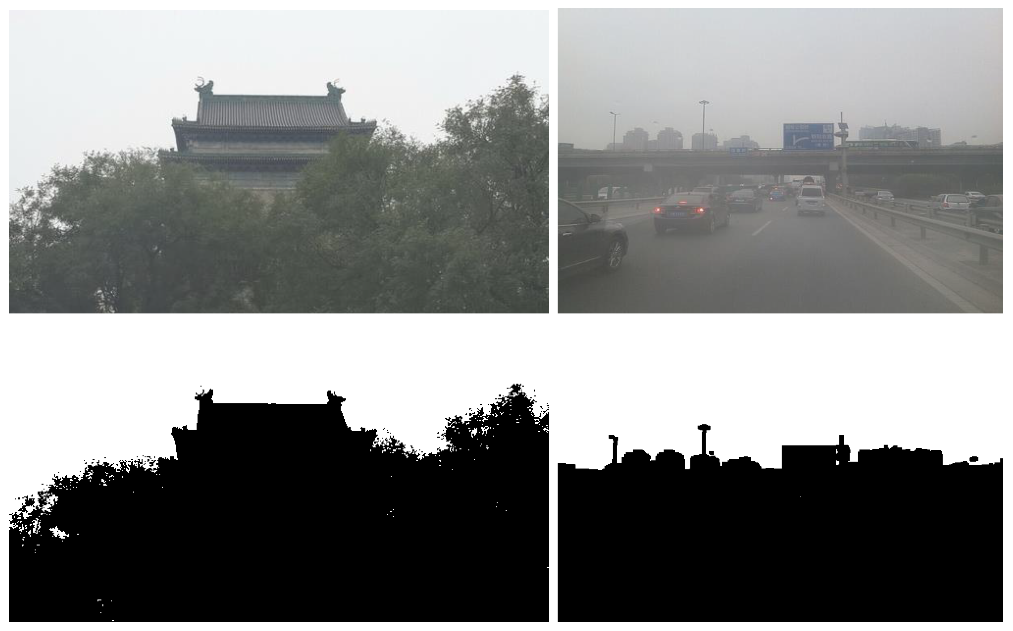
  • A Otsu and PSO method is proposed to accurately segment the sky and non-sky regions of hazy images, which allows the different priors in the two regions to estimate the parameters accurately.
  • We propose an improved BCP to more accurately estimate the transmission map. Inaccurate estimation of the parameters of the sky region can easily amplify noise and cause distortion, so we limit it.
  • To better fuse the parameters estimated by BCP and DCP, we propose weighted fusion functions to obtain more accurate transmission maps and atmospheric light values, respectively.

2. Related Work

2.1. Image-Enhancement-Based Methods

Methods based on image enhancement include histogram equalization and the Retinex algorithm. The histogram equalization dehazing method is to transform the gray value of the hazy image into a uniform distribution. Retinex is a color vision model [1]. Differently from traditional methods, Retinex can adaptively enhance various images. However, since the dehazing is not performed physically, such methods are not robust.

2.2. Prior-Based Methods

Low visibility in hazy weather is affected by atmospheric particles. The most common ASM is to describe the image degradation process in hazy weather:
I ( q ) = J ( q ) t ( q ) + A ( 1 t ( q ) )
where q represents the position of a pixel, I ( q ) denotes the hazy image, J ( q ) represents the clear image, A is the global atmospheric light and t ( q ) is the transmission map. The task of image dehazing is to restore J ( q ) from I ( q ) . Some scholars propose prior knowledge to estimate J ( q ) . The DCP-based algorithm [7] is the first method to combine DCP with ASM for image dehazing. The mathematical expression of the dark channel:
J d a r k ( q ) = m i n y Ω ( q ) ( m i n c ( R , G , B ) J c ( q ) ) , J d a r k ( q ) 0
where c is a channel combining the three channels of R, G, and B; J d a r k ( q ) can be calculated by replacing the gray value of the center point pixel with the minimum gray value in the rectangular area Ω ( q ) . According to DCP theory, J d a r k ( q ) is close to zero. DCP is introduced to estimate the values of t ( q ) and A, and DCP has become the fastest-growing and most widely used image dehazing algorithm. Therefore, many scholars have proposed a large number of improved algorithms based on DCP [34,35,36,37]. However, many DCP-based works cannot provide the dehazing of the sky region and are prone to halo and distortion, and the use of algorithms has high requirements for light intensity. Zhu [38] proposed a color attenuation prior based on the statistical analysis of a large number of hazy images. The method shows that the higher the haze concentration, the larger the depth of field. He et al. [39] converted the parameter estimation into a convex linear optimization problem and introduced the Haar wavelet transform to speed up the solution. It provides good real-time performance. Ehsan [40] proposed a dual-transmission map method to restore the haze-free image and reduce the halo phenomenon.

2.3. Learning-Based Methods
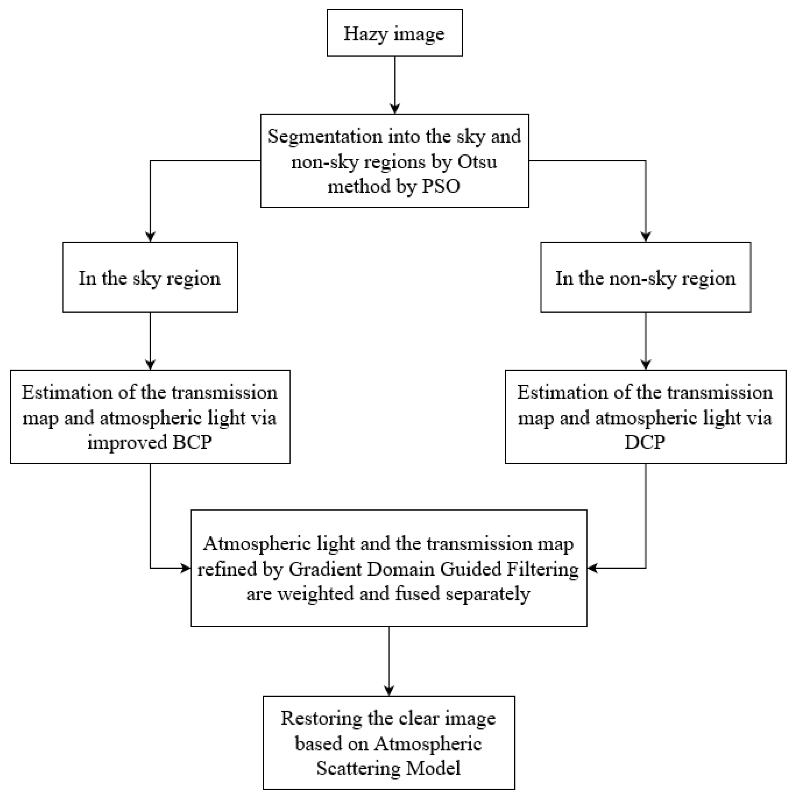
There is also a large number of learning-based methods in the field of haze removal. Cai [41] proposed DehazeNet that can directly estimate the transmission map and then completed the reconstruction of the clear image according to ASM. DehazeNet combines the prior knowledge of the traditional dehazing network and obtains refined transmission maps through feature extraction and nonlinear regression, and guided filtering [42]. DehazeNet’s dehazing effect is good, but there are certain problems. Due to the different degrees of light absorption, scattering, and transmission in different locations in the real atmospheric environment, the distribution of atmospheric light is uneven, and the atmospheric light obtained by using an assumptions prior cannot be well adapted to various situations in the dehazing task. The processing effect at the change of depth of field is average. Ren [15] proposed a single-image dehazing network (MSCNN), which first estimated the overall transmission map and then further optimized it, and then analyzed the difference between the features acquired by traditional methods and convolutional neural network learning. Li [14] proposed AOD-Net, which unifies the two parameters in ASM into one parameter through the conversion formula, eliminating intermediate steps and reducing the cumulative error in parameter estimation. The network consists of two sub-modules, which are simple in structure and efficient in processing. Engin [43] proposed an enhanced cycle generation adversarial network (Cycle-Dehaze) that can directly generate a haze-free image without estimating the parameters of ASM and in an unpaired manner. The network combines with perceptual loss to improve the cycle consistency loss of CycleGAN architecture. Chen [44] proposed GCANet, which used a smooth dilation technique that inserts dilated residual blocks between codecs to aggregate contextual information without causing grid artifacts. Wu [45] proposed AECR-Net based on contrastive learning, which uses the information of clear images and hazy images as positive samples and negative samples respectively, ensuring that the restored result images are closer to clear images. The network introduces deformable convolution into the dynamic feature enhancement module in AECR-Net so that the sampling grid can dynamically adapt to the shape to expand the receiving field and achieve a better dehazing effect. AECR-Net is based on an autoencoder-like framework, which becomes more compact by reducing the number of layers and the size of the space. Tran et al. [46] proposed a new encoding–decoding network (EDN-GTM) that uses traditional RGB hazy images and transmission maps estimated using dark channel priors as input to the network, U-Net as the core network for image processing, and the spatial pyramid pooling module and the Swish activation function in the network to achieve a better dehazing goal. Zhao [47] proposed a nighttime image dehazing network, which fuses three inputs through white balance. Alenezi [48] proposed an underwater image dehazing network that utilizes the color channels and image features of RGB images to improve overall usability. The output color channel features are fused using softmax weighting to obtain a clear image. Yang [49] proposed a self-enhanced image dehazing framework D4 that focuses on the scattering coefficient and depth information of images. They trained the network through unpaired hazy and clear images to restore the scattering coefficient, depth map, and clear images. Song et al. proposed DehazeFormer [50], which improved the structure of Swin Transformer [51] to make it more suitable for the dehazing task. Song et al. proposed a compact dehazing network gUNet [52] based on UNet [53] and achieved good results. Despite the great success of deep learning-based methods, their generalization performance is unsatisfactory due to heavy reliance on synthetic hazy image datasets.

3. Methods

The method we propose mainly consists of three steps. We first segment the sky region of the hazy image. Then, we estimate the transmission map and atmospheric light via the proposed improved BCP and DCP. Finally, we fuse the transmission map and atmospheric light and restore the clear image. The overall flowchart is shown in Figure 1.

3.1. Otsu Method by Particle Swarm Optimization

We propose an Otsu method [54,55] that uses particle swarm optimization (PSO) [56,57] to find a better segmentation threshold to separate the sky region from the non-sky regions in hazy images. The Otsu method by PSO can more accurately segment the sky and non-sky regions.
We first convert the RGB hazy image into a grayscale image, letting N U M represent the total number of pixels of the image and c o u n t ( x ) the number of pixels with a pixel gray value of x. Then, the number of pixels with a gray value of x that appears in the image probability P ( x ) can be expressed as:
P ( x ) = c o u n t ( x ) N U M , 0 255 P ( x ) = 1
Assuming that t is the threshold value for segmenting the non-sky and sky region of the image, the pixels with gray values ranging from 0 to t are classified as non-sky regions, and the pixels with gray values ranging from t + 1 to 255 are classified as sky regions. Let w 1 and w 2 denote the probabilities of two regions:
w 1 = x = 0 t P ( x ) , w 2 = x = t + 1 255 P ( x )
Then, get the mean u 1 and u 2 of the two regions:
u 1 = x = 0 t x × P ( x ) w 1 , u 2 = x = t + 1 255 x × P ( x ) w 2
Then, the mathematical expectation of the overall pixel gray value of the image is:
u = w 1 × u 1 + w 2 × u 2
According to the OSTU method [58], the optimal threshold t can be obtained by maximizing the between-cluster variance σ 2 of the image:
σ 2 = w 1 × ( u 1 u ) 2 + w 2 × ( u 2 u ) 2
Then, we use Equation (7) as the fitness function of PSO. We used 500 particles and iterated 400 times to adaptively obtain the optimal segmentation threshold t. Finally, we performed binarization processing and set the pixel value of the sky region whose gray value is greater than the threshold t to 1, and the pixel value of the non-sky area whose gray value is less than or equal to the threshold t to be 0. Figure 2 shows the effect of segmentation.

3.2. Accurate Estimation of Transmission Map and Atmospheric Light

3.2.1. In the Non-Sky Region

In the non-sky regions, DCP performs very well, so we use DCP for the initial estimation. From Equations (1) and (2), the transmission map estimated by DCP [7] is:
t _ D C P ( q ) = 1 ω m i n y Ω ( q ) ( m i n c I c ( y ) A D C P c )
where the parameter ω is used to make distant objects have a small amount of haze, which was set to 0.95 in [7]. As for the estimation of atmospheric light A D C P , we also use the method of He [7]. First, we select the 0.1% brightest pixels in the dark channel and then take the average value of the pixel values in the corresponding input image as the estimated value of atmospheric light.

3.2.2. In the Sky Region

Since DCP fails in the sky region [7], we adopt the improved BCP to estimate parameters in the sky region. According to the BCP theory [33], the intensity values of most images containing white objects or light sources in the RGB color channel are particularly large, or even close to 255. For an image J ( q ) , the mathematical expression of the bright channel is:
J b r i g h t ( q ) = m a x y Ω ( q ) m a x c ( R , G , B ) ) [ J c ( q ) ] , J b r i g h t ( q ) 255
where c is a channel combining the three channels of R, G, and B; Ω ( q ) is a rectangular area centered at q. According to the BCP theory, J b r i g h t ( q ) is close to 255. From ASM (Equation (1)) and BCP (Equation (9)), it can be deduced that the transmission map is:
t _ b r i g h t ( q ) = m a x [ m a x y Ω ( p ) I c ( y ) ] A b r i g h t c 255 A b r i g h t c
where c is a channel combining the three channels of R, G, and B; Ω ( q ) is a rectangular area centered at q. However, the transmission map obtained in this way may be a negative value or may be too small, so we improved it. We let b = m a x m a x y Ω ( q ) I c ( y ) A b r i g h t c , and m e a n ( b ) represents the mean of b. Then:
t _ b r i g h t ( q ) = b + k 255 A b r i g h t c , i f b < m e a u ( b ) b 255 A b r i g h t c , i f b m e a u ( b )
where k is the adjustment factor, and it was found through experiments that the value of k is most suitable between 0.05 and 0.15. In addition, in order to prevent the transmission map of pixels from exceeding 1, we made another restriction as follows:
t _ b r i g h t ( q ) = m i n t _ b r i g h t ( q ) , 1
For the estimation of atmospheric light A b r i g h t based on BCP, according to the BCP, the maximum value of the bright channel in the region where the atmospheric light is located is closest to the atmospheric light, so we take the 0.1-percent brightest pixels of the bright channel and then take the average value of the pixel of the corresponding input image as the atmospheric light estimated value.

3.3. Fusion of Sky and Non-Sky Regions

In order to better fuse the estimated parameters of the sky and non-sky region, we propose a more appropriate weighted fusion function.

3.3.1. Transmission Map Fusion

According to the DCP and BCP theories, the transmission map estimated by DCP is suitable for non-sky regions, and the transmission map estimated by BCP is suitable for sky regions. For better fusion, we introduce a weight parameter λ :
λ = Z H × W
where Z represents the total number of pixels in the sky region, which can be obtained by calculating the number of pixels whose pixel value is [t + 1, 255]; H and W represent the height and width of the image, respectively; H × W represents the total number of pixels of the image. The fused transmission map t ( q ) is:
t ( q ) = λ t _ b r i g h t ( q ) + ( 1 λ ) t _ d a r k ( q ) σ
where σ = 1 10 e Z H × W Z 0.05 is an adaptive parameter we designed, and the value of σ belongs to [−0.05, 0.05]; Z is the total number of pixels in the sky region; ( H × W Z ) is the total number of pixels in the non-sky region; the value of σ in the sky region is a negative number; and the value of σ in the non-sky region is a positive number. The fused transmission map t ( q ) is then refined by gradient domain guided filtering [59] to reduce blocking artifacts. Experiments verify that the transmission map obtained after σ fine-tuning can make the image recovery better.

3.3.2. Atmospheric Light Fusion

Since the atmospheric light obtained by the bright channel has an atmospheric light value near to that of light in the haze-free state, we fuse the atmospheric light as follows:
A = λ A D C P + ( 1 λ ) A b r i g h t

3.4. Recovering the Clear Image

According to Equation (1), the final recovered clear image J ( p ) is as follows:
J ( q ) = I ( q ) A m a x ( t ( q ) , 0.1 ) + A
where we set a lower limit of 0.1 for the transmission map, retaining a little haze and preventing noise amplification caused by the too-small transmission map. The algorithm of the proposed method is described in Algorithm 1.
Algorithm 1: Single image dehazing based on improved BCP and DCP.
Input: A hazy image I ( q )
(1) Segmentation I ( q ) into sky area and non-sky regions using OSTU by PSO.
(2.1) For the non-sky region of I ( q ) , the transmission map t _ D C P ( q ) and atmospheric light A D C P are estimated by DCP.
(2.2) For the sky region of I ( q ) , the transmission map t _ b r i g h t ( q ) and atmospheric light A b r i g h t are estimated by improved BCP.
(3) Fuse t _ D C P ( q ) and t _ b r i g h t ( q ) by Equation (14), and fuse A D C P and A b r i g h t by Equation (15)
(4) Recovering the clear image J ( q ) byEquation (16)
Output: The clear image J ( q )

4. Experiments and Discussion

We randomly sampled some images from the synthetic hazy image (RESIDE dataset [60]) and real hazy images (O-Haze dataset [61] and NH-Haze dataset [62]) for comparative experiments, and used the peak-signal-to-noise ratio (PSNR) and the structural similarity index measure (SSIM) metrics [63] for quantitative evaluation. We conducted detailed comparative experiments with state-of-the-art methods, including DCP [7], BCCR [9], NonLocal [10], MSCNN [15], DehazeNet [41], AODNet [14], He [39], Ehsan [40], D4 [49], DehazeFormer-T [50], and gUNet-T [52].

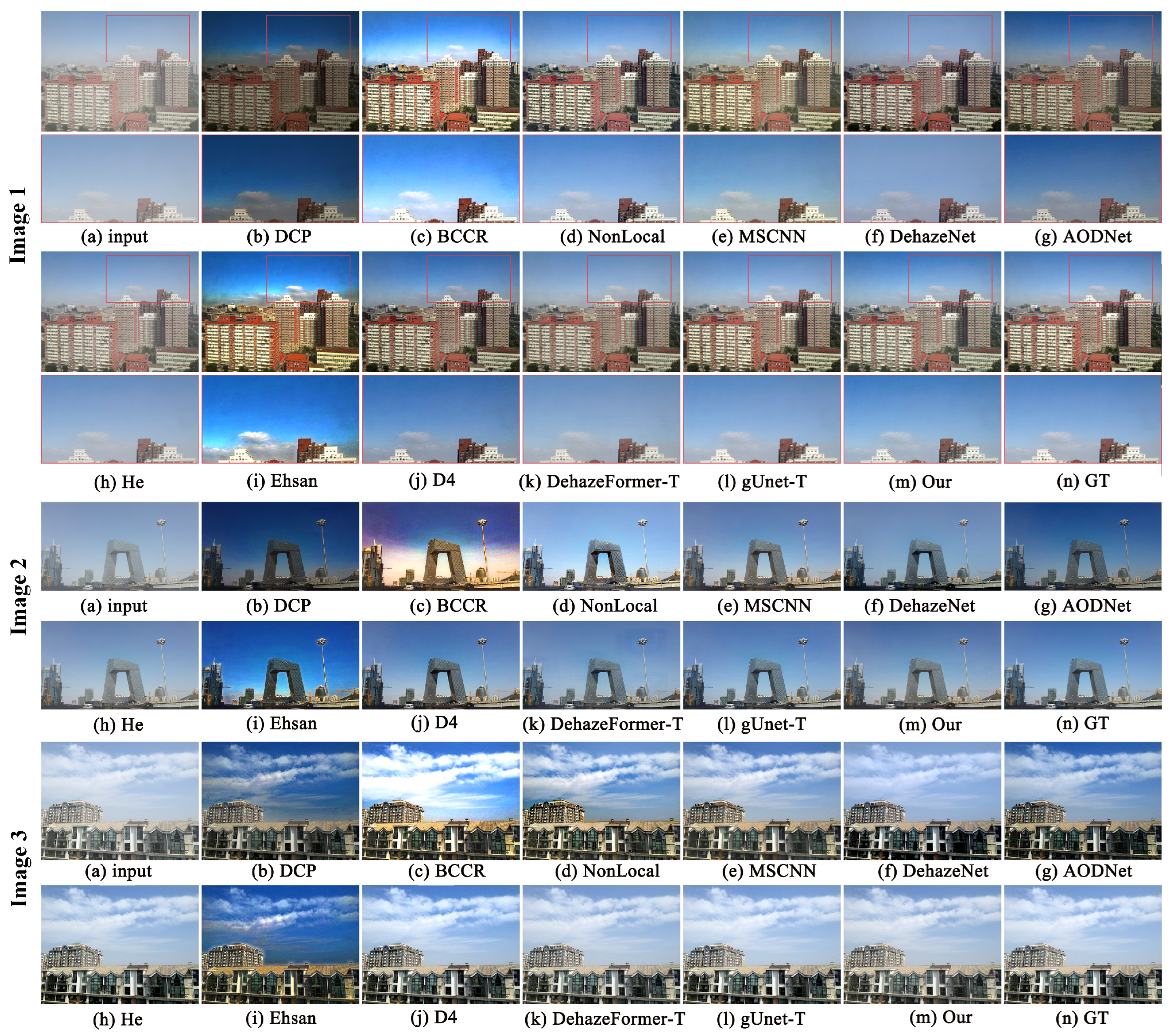
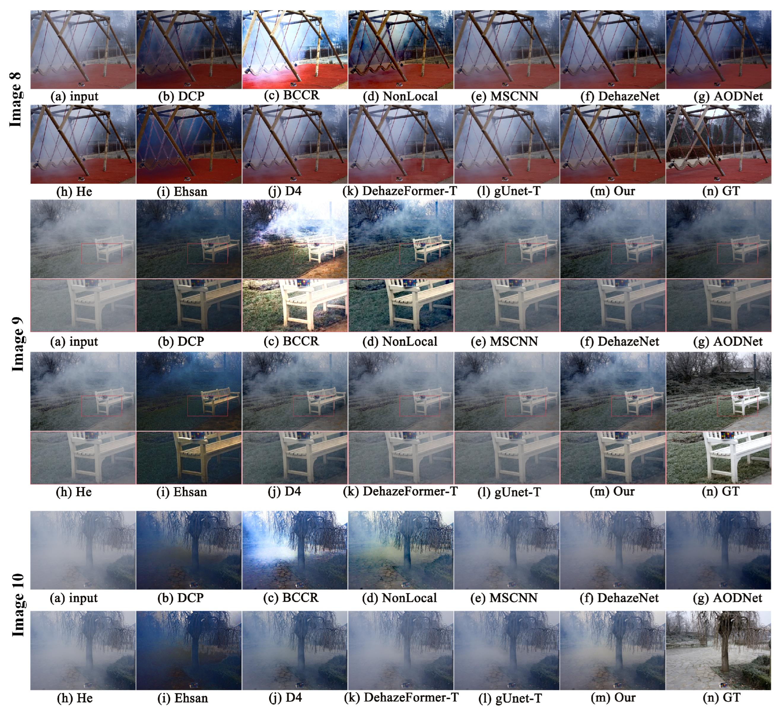
4.1. Experiments on Synthetic Hazy Images

We randomly sampled several images from SOTS-Outdoor (from RESIDE dataset) for experimental comparison. The visual comparison is shown in Figure 3. For Image 1, the result of restoration via DCP is overall darker; the image restored by BCCR is a bit overexposed; the result of restoration by He’s method has more haze; the color restoration result of AODNet and Ehsan’s method shows a great change; the result of restoration by NonLocal, MSCNN, DehazeNet, and D4 has color distortion; the result of restoration by our method is closest to ground truth (GT)—the sky area is very well protected. For Image 2 and Image 3, the restored results of DCP, BCCR, AODNet, and Ehsan show severe color distortion. He’s method was not effective in dehazing, and the restored results of NonLocal, MSCNN, DehazeNet, and D4 show overexposure or overexposure in the sky region. The overall restoration effects of DehazeFormer-T and gUNet-T are better, but the restoration results of the sky region in Image 1 are slightly different from those of GT. The result recovered by our method is closest to that of GT. The comparison of visual effect experiments shows that our method can well protect the sky region of the image, which solves the problem that DCP fails in the sky region.

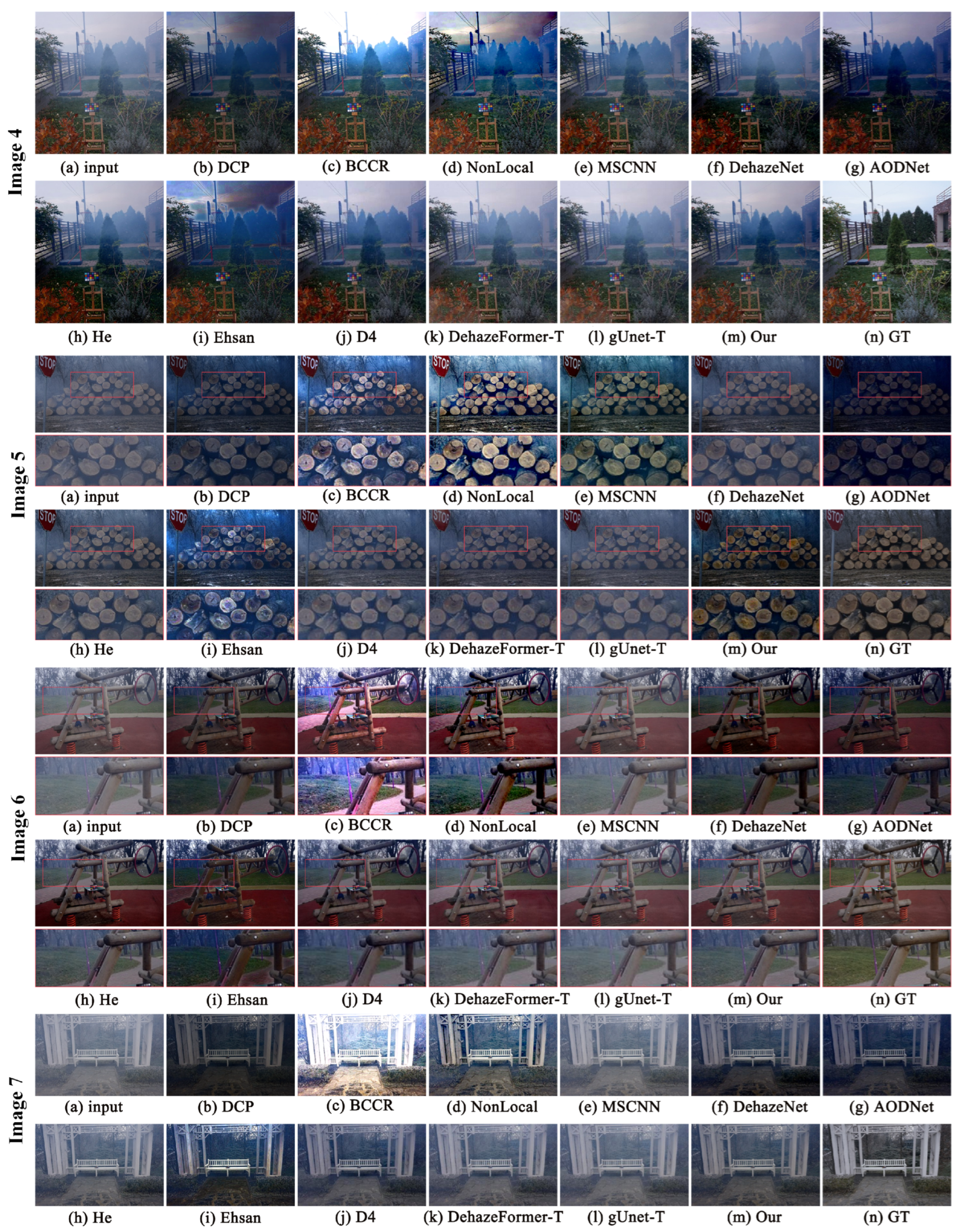
4.2. Experiments on Real-World Hazy Images

We randomly sampled several images from the O-Haze and NH-Haze datasets for comparative experiments. Both O-Haze and NH-Haze datasets show haze generated by professional haze generators. O-Haze has hazy outdoor scenes, and NH-Haze has uneven haze. Figure 4 shows the dehazing effects of different methods on the O-Haze dataset. In Image 4 of Figure 4, the results restored by DCP, NonLocal, and Ehsan methods are severely distorted in the sky region, and the result of BCCR is that the sky area is overexposed. The results of restoration by DehazeNet, MSCNN, He, D4, DehazeFormer-T, and gUNet-T have more haze, as shown in the tree area in Image 4. The result of recovery by AODNet is oversaturated. For Image 5, the BCCR and NonLocal methods increased the original brightness, and AODNet reduced the original brightness of the image. The result recovered by Ehsan’s method is severely distorted. The results of D4, DehazeFormer-T, and gUNet-T restoration still show residual haze, such as the red box area. For Image 6, the recovery results of DCP, DehazeNet, AODNet, and Ehsan are all darker, and the brightness of the recovery result of BCCR is obviously changed. The recovery by MSCNN, DehazeFormer-T, and gUnet-T left the haze visible to the naked eye, such as the grass part of the image. Image 7 shows a similar result. The results recovered by our method have the least haze while being closest to GT.
Figure 5 is a comparison on the NH-Haze dataset. The haze in each image in this dataset is relatively thick. The images restored by methods such as DCP, AODNet, and Ehsan are too dark or oversaturated. The image recovered by BCCR is overexposed. The images restored by MSCNN, DehazeNet, He, and D4 methods still have more haze; and the images restored by NonLocal have less haze, as shown in Image 8, which may be because the non-local prior has a better dehazing effect on uneven haze, but the scene color shows some distortion. In Image 9, the results recovered by DCP and Ehsan are darker; the result of BCCR is overexposed; and the results recovered by MSCNN, He, DehazeFormer-T, and gUnet-T have more residual haze, such as the area shown in the red box. The scene details restored by NonLocal feel good, but the color of the haze is changed, making it the same in Image 10. The image restored by our method is relatively closer to GT in terms of color and saturation, but there is still a certain amount of haze, which is where our future work can be improved.

4.3. Quantitative Evaluation Experiment

To objectively verify the performance, we conducted a detailed quantitative evaluation using PSNR and SSIM metrics for comparison. Table 1 is the quantitative experimental comparison results of all images in Figure 3, Figure 4 and Figure 5. In Table 1, the highest PNSR/SSIM scores of Image 1, Image 2, and Image 3 are based on the deep learning method gUNet, which is due to the fact that gUNet learns better features on synthetic data. However, the PNSR/SSIM score of our method was the highest on the remaining real-world hazy images, which illustrates the excellent performance of our method in real-world scenes.
In addition, we performed quantitative comparison experiments on all images on the SOTS-Outdoor dataset, O-Haze dataset, and NH-Haze dataset. Table 2 shows the average PNSR/SSIM score results of the three datasets. On the synthetic data, SOTS-Outdoor, our method, scored inferiorly to the latest deep learning methods DehazeFormer-T and gUNet-T, which shows that these two methods perform well on synthetic datasets. However, our method scored the highest on the O-Haze and NH-Haze datasets of real-world hazy images, which further illustrates the excellent dehazing performance of our method in the real world. The performance of deep learning-based methods on real-world images is inferior to that of our method, possibly due to the overfitting of models trained on synthetic datasets. This also shows that deep learning-based methods may have poor generalization ability due to their heavy dependence on datasets.

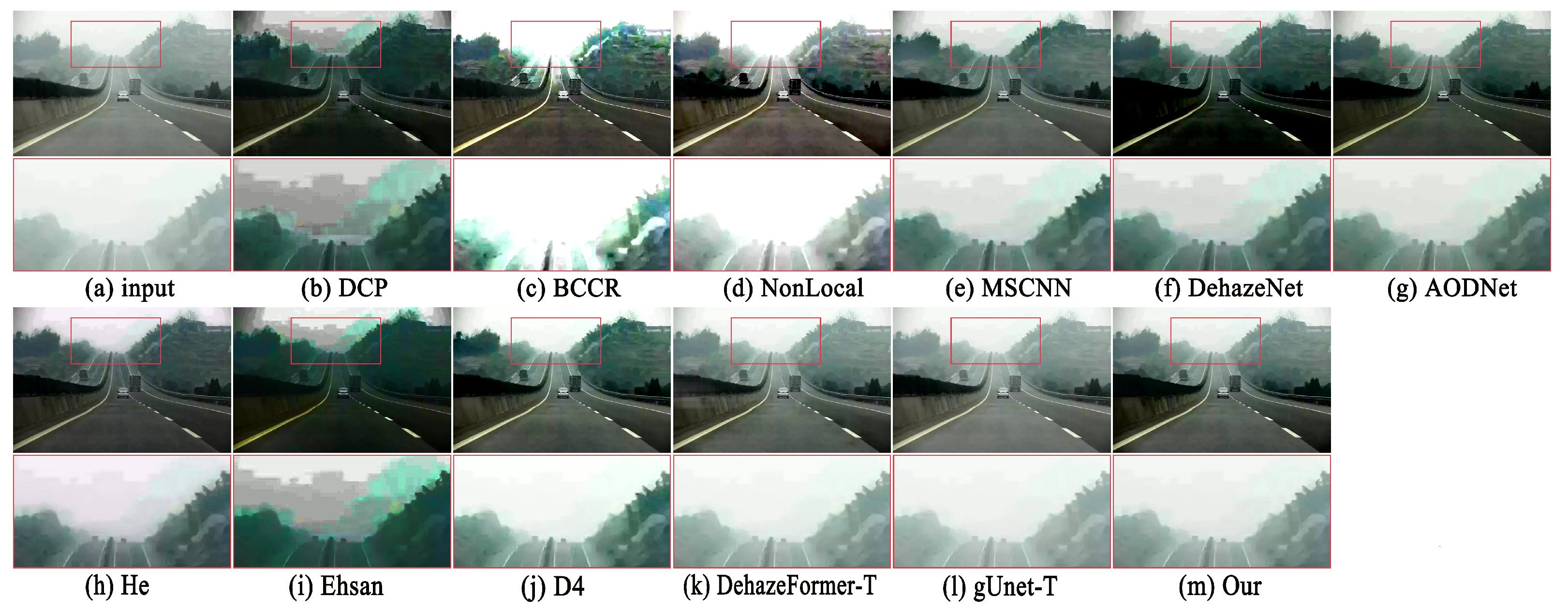
4.4. Application in Traffic Electronic Monitoring

On roads, especially in mountainous areas, haze is prone to occur, and there is much electronic monitoring on roads. Hazy weather may affect the collection of vehicle information by electronic monitoring, such as vehicle color, license plate number, and other information. Our method can also be used for haze removal in hazy images collected by traffic electronic monitoring. We downloaded a hazy traffic scene from the Internet and conducted a comparative experiment. As shown in Figure 6, the results recovered by DCP, BCCR, and Ehsan methods has obvious color distortion. The sky region of the NonLocal restored result is overexposed. The results recovered by MSCNN, DehazeNet, AODNet, and He have distortion in the sky region; and the road part recovered by DehazeNet, AODNet, He, Ehsan, and D4 is too dark. The overall effects of the DehazeFormer-T and gUnet-T restoration are superior, but there will be more residual haze, whereas the restoration result of our method reduces distortion while removing haze. Since there is no GT image, it is impossible to quantitatively evaluate the PNSR/SSIM index, but we used a fog aware density evaluator (FADE) [53] to measure the amount of haze. The score of the FADE index indicates the density of haze to a certain extent. In Table 3, the haze density of the image recovered by the DehazeNet method is shown to be the smallest, which reflects that the method has good dehazing ability, but the visual effect is not satisfactory. Our method restores the image fog concentration only 0.024 more than the DehazeNet method. The FADE value of the image recovered by our method is only 0.024 higher than that of the DehazeNet method, which shows that the dehazing performance by our method is also very good. In addition, it can be seen that the images recovered by MSCNN, DehazeFormer-T, and gUNet-T methods have more residual haze, which illustrates the limitations of these methods for dehazing.

4.5. Processing Time of the Algorithm

We used MATLAB 2019a software to execute our algorithm on an Intel i7-7700 3.6 GHz CPU and 8 GB RAM environment to obtain the haze-free images. Table 4 shows the processing times of all images in Figure 3, Figure 4 and Figure 5. In Table 4, we can see that as the size of the image increases, the processing time of the algorithm increases. Especially for high-definition images with a resolution of 1600 × 1200, the algorithm’s processing time increases significantly. The two most time-consuming operations of the algorithm are to use PSO to find the optimal segmentation threshold t and to traverse each pixel of the image to determine whether it belongs to the sky region. This shows that our method takes more time to process high-definition images, which is also the direction of our future improvement.

5. Conclusions

We propose a simple yet effective dehazing method. In order to solve the famous DCP failure in the sky region, we segment the sky area of the image, use the improved BCP to estimate the parameter in the sky area, and use DCP to estimate the transmission map in the non-sky area and atmospheric light. We then efficiently fuse the parameters of the two regions, and then recover a clear image according to ASM. We conducted visual and quantitative comparison experiments on synthetic and real-world datasets with state-of-the-art methods. The results demonstrate that our method can well preserve sky regions, reduce color distortion and oversaturation, and provide higher PSNR and SSIM scores. Recent learning-based methods have achieved excellent performance on synthetic datasets due to their powerful backbone networks for learning image features, such as UNet and Swin transformer. However, the learning-based method has poor generalization ability due to its heavy dependence on the specific dataset it is trained with, and it may not perform satisfactorily on new scenes. In contrast, our method is unsupervised and performs well in real-world scenarios, which illustrates the effectiveness of physical models and prior knowledge.
In addition, the proposed method cannot fully achieve the effect of dehazing non-uniform thick hazy images, which may be due to the fact that the physical model and prior knowledge are not fully practical in non-uniform haze scenes, which is also the direction of our future work. In the future, we will try to study a more robust physical model that can reflect the imaging process of images with various haze concentrations.

Author Contributions

Writing—original draft preparation, C.L.; writing—review and editing, H.X. and H.Z.; supervision, H.X.; experiment, C.Y., H.P., Y.Y. and Z.W.; funding acquisition, H.X. All authors have read and agreed to the published version of the manuscript.

Funding

This work was supported by the Science and Technology Research Program of Chongqing Municipal Education Commission (grant No. KJQN202102002; NO. KJZD-K202102001), the Science and Technology Research Plan of Chongqing Education Commission (No.: KJQN201903311), the National College Students’ innovation and entrepreneurship training program of China (grant No. 202211306020), and the Fundamental Research Funds for the Central Universities of China (SWU2009107).

Institutional Review Board Statement

This paper does not studies not involving humans or animals.

Informed Consent Statement

This paper does not studies not involving humans or animals.

Conflicts of Interest

The authors declare no conflict of interest.

References

  1. Li, H.; Xie, W.H.; Wang, X.G.; Liu, S.S.; Gai, Y.Y.; Yang, L. Gpu implementation of multi-scale retinex image enhancement algorithm. In Proceedings of the 2016 IEEE/ACS 13th International Conference of Computer Systems and Applications (AICCSA), Agadir, Morocco, 29 November–2 December 2016; pp. 1–5. [Google Scholar]
  2. Kim, W.; You, J.; Jeong, J. Contrast enhancement using histogram equalization based on logarithmic mapping. Opt. Eng. 2012, 51, 067002. [Google Scholar] [CrossRef]
  3. Laha, S.; Foroosh, H. Haar Wavelet-Based Attention Network for Image Dehazing. In Proceedings of the 2022 IEEE International Conference on Image Processing (ICIP), Bordeaux, France, 16–19 October 2022; pp. 3948–3952. [Google Scholar]
  4. Middleton, W.E.K.; Twersky, V. Vision through the atmosphere. Phys. Today 1954, 7, 21. [Google Scholar] [CrossRef]
  5. McCartney, E.J. Optics of the atmosphere: Scattering by molecules and particles. Phys. Today 1976, 30, 76. [Google Scholar] [CrossRef]
  6. Narasimhan, S.G.; Nayar, S.K. Vision and the atmosphere. Int. J. Comput. Vis. 2002, 48, 233–254. [Google Scholar] [CrossRef]
  7. He, K.M.; Sun, J.; Tang, X.O. Single image haze removal using dark channel prior. IEEE Trans. Pattern Anal. Mach. Intell. 2011, 33, 2341–2353. [Google Scholar] [PubMed]
  8. Zhou, H.; Zhang, Z.; Liu, Y.; Xuan, M.; Jiang, W.; Xiong, H. Single Image Dehazing Algorithm Based on Modified Dark Channel Prior. IEICE Trans. Inf. Syst. 2021, 104, 1758–1761. [Google Scholar] [CrossRef]
  9. Meng, G.F.; Wang, Y.; Duan, J.Y.; Xiang, S.M.; Pan, C.H. Efficient image dehazing with boundary constraint and contextual regularization. In Proceedings of the IEEE International Conference on Computer Vision, Sydney, NSW, Australia, 1–8 December 2013; pp. 617–624. [Google Scholar]
  10. Berman, D.; Treibitz, T.; Avidan, S. Non-local image dehazing. In Proceedings of the IEEE Conference on Computer Vision and Pattern Recognition, Las Vegas, NV, USA, 27–30 June 2016; pp. 1674–1682. [Google Scholar]
  11. Zhou, H.; Xiong, H.; Li, C.; Jiang, W.; Lu, K.; Chen, N.; Liu, Y. Single image dehazing based on weighted variational regularized model. IEICE Trans. Inf. Syst. 2021, 104, 961–969. [Google Scholar] [CrossRef]
  12. Zhou, H.; Zhao, Z.; Xiong, H.; Liu, Y. A unified weighted variational model for simultaneously haze removal and noise suppression of hazy images. Displays 2022, 72, 102137. [Google Scholar] [CrossRef]
  13. Hsieh, P.W.; Shao, P.C. Variational contrast-saturation enhancement model for effective single image dehazing. Signal Process. 2022, 192, 108396. [Google Scholar] [CrossRef]
  14. Li, B.; Peng, X.; Wang, Z.Y.; Xu, D.; Feng, J.Z. Aod-net: All-in-one dehazing network. In Proceedings of the IEEE International Conference on Computer Vision, Venice, Italy, 22–29 October 2017; pp. 4780–4788. [Google Scholar]
  15. Ren, W.; Liu, S.; Zhang, H.; Pan, J.; Cao, X.; Yang, M.H. Single image dehazing via multi-scale convolutional neural networks. In Proceedings of the European Conference on Computer Vision, Amsterdam, The Netherlands, 11–14 October 2016; pp. 154–169. [Google Scholar]
  16. Li, S.; Yuan, Q.; Zhang, Y.; Lv, B.; Wei, F. Image Dehazing Algorithm Based on Deep Learning Coupled Local and Global Features. Appl. Sci. 2022, 12, 8552. [Google Scholar] [CrossRef]
  17. Liu, Y.; Zhu, L.; Pei, S.; Fu, H.; Qin, J.; Zhang, Q.; Wan, L.; Feng, W. From synthetic to real: Image dehazing collaborating with unlabeled real data. In Proceedings of the 29th ACM International Conference on Multimedia, Virtual, 20–24 October 2021; pp. 50–58. [Google Scholar]
  18. Liu, Y.; Wan, L.; Fu, H.; Qin, J.; Zhu, L. Phase-based Memory Network for Video Dehazing. In Proceedings of the 30th ACM International Conference on Multimedia, Lisbon, Portugal, 10–14 October 2022; pp. 5427–5435. [Google Scholar]
  19. Yu, H.; Zheng, N.; Zhou, M.; Huang, J.; Xiao, Z.; Zhao, F. Frequency and Spatial Dual Guidance for Image Dehazing. In Proceedings of the European Conference on Computer Vision, Tel Aviv, Israel, 23–27 October 2022; pp. 181–198. [Google Scholar]
  20. Zhang, J.; He, F.; Duan, Y.; Yang, S. AIDEDNet: Anti-interference and detail enhancement dehazing network for real-world scenes. Front. Comput. Sci. 2023, 17, 1–11. [Google Scholar] [CrossRef]
  21. Wu, Y.; Tao, D.; Zhan, Y.; Zhang, C. BiN-Flow: Bidirectional Normalizing Flow for Robust Image Dehazing. IEEE Trans. Image Process. 2022, 31, 6635–6648. [Google Scholar] [CrossRef] [PubMed]
  22. Bai, H.; Pan, J.; Xiang, X.; Tang, J. Self-guided image dehazing using progressive feature fusion. IEEE Trans. Image Process. 2022, 31, 1217–1229. [Google Scholar] [CrossRef]
  23. Sahu, G.; Seal, A.; Yazidi, A.; Krejcar, O. A Dual-Channel Dehaze-Net for Single Image Dehazing in Visual Internet of Things Using PYNQ-Z2 Board. IEEE Trans. Autom. Sci. Eng. 2022. [Google Scholar] [CrossRef]
  24. Susladkar, O.; Deshmukh, G.; Nag, S.; Mantravadi, A.; Makwana, D.; Ravichandran, S.; Chavhan, G.H.; Mohan, C.K.; Mittal, S. ClarifyNet: A high-pass and low-pass filtering based CNN for single image dehazing. J. Syst. Archit. 2022, 132, 102736. [Google Scholar] [CrossRef]
  25. Jiang, N.; Hu, K.; Zhang, T.; Chen, W.; Xu, Y.; Zhao, T. Deep Hybrid Model for Single Image Dehazing and Detail Refinement. Pattern Recognit. 2022, 136, 109227. [Google Scholar] [CrossRef]
  26. Meng, J.; Li, Y.; Liang, H.; Ma, Y. Single-image dehazing based on two-stream convolutional neural network. J. Artif. Intell. Technol. 2022, 2, 100–110. [Google Scholar] [CrossRef]
  27. Chen, X.; Fan, Z.; Li, P.; Dai, L.; Kong, C.; Zheng, Z.; Huang, Y.; Li, Y. Unpaired Deep Image Dehazing Using Contrastive Disentanglement Learning. In Proceedings of the European Conference on Computer Vision, Tel Aviv, Israel, 23–27 October 2022; pp. 632–648. [Google Scholar]
  28. Zheng, Y.; Su, J.; Zhang, S.; Tao, M.; Wang, L. Dehaze-AGGAN: Unpaired Remote Sensing Image Dehazing Using Enhanced Attention-Guide Generative Adversarial Networks. IEEE Trans. Geosci. Remote Sens. 2022, 60, 1–13. [Google Scholar] [CrossRef]
  29. Alenezi, F.; Armghan, A.; Santosh, K. Underwater image dehazing using global color features. Eng. Appl. Artif. Intell. 2022, 116, 105489. [Google Scholar] [CrossRef]
  30. Hassan, H.; Mishra, P.; Ahmad, M.; Bashir, A.K.; Huang, B.; Luo, B. Effects of haze and dehazing on deep learning-based vision models. Appl. Intell. 2022, 52, 16334–16352. [Google Scholar] [CrossRef]
  31. Parihar, A.S.; Java, A. Densely connected convolutional transformer for single image dehazing. J. Vis. Commun. Image Represent. 2022, 90, 103722. [Google Scholar] [CrossRef]
  32. Zheng, L.; Li, Y.; Zhang, K.; Luo, W. T-Net: Deep stacked scale-iteration network for image dehazing. IEEE Trans. Multimed. 2022. [Google Scholar] [CrossRef]
  33. Yan, Y.; Ren, W.; Guo, Y.; Wang, R.; Cao, X. Image deblurring via extreme channels prior. In Proceedings of the IEEE Conference on Computer Vision and Pattern Recognition, Honolulu, HI, USA, 21–26 July 2017; pp. 4003–4011. [Google Scholar]
  34. Cao, N.; Lyu, S.; Hou, M.; Wang, W.; Gao, Z.; Shaker, A.; Dong, Y. Restoration method of sootiness mural images based on dark channel prior and Retinex by bilateral filter. Herit. Sci. 2021, 9, 1–19. [Google Scholar] [CrossRef]
  35. Wang, M.-w.; Zhu, F.-z.; Bai, Y.-y. An improved image blind deblurring based on dark channel prior. Optoelectron. Lett. 2021, 17, 40–46. [Google Scholar] [CrossRef]
  36. Pan, Y.; Chen, Z.; Li, X.; He, W. Single-Image Dehazing via Dark Channel Prior and Adaptive Threshold. Int. J. Image Graph. 2021, 21, 2150053. [Google Scholar] [CrossRef]
  37. Wang, Y.; Huang, T.Z.; Zhao, X.L.; Deng, L.J.; Ji, T.Y. A convex single image dehazing model via sparse dark channel prior. Appl. Math. Comput. 2020, 375, 125085. [Google Scholar] [CrossRef]
  38. Zhu, Q.; Mai, J.; Shao, L. A fast single image haze removal algorithm using color attenuation prior. IEEE Trans. Image Process. 2015, 24, 3522–3533. [Google Scholar]
  39. He, J.; Xing, F.Z.; Yang, R.; Zhang, C. Fast single image dehazing via multilevel wavelet transform based optimization. arXiv 2019, arXiv:1904.08573. [Google Scholar]
  40. Ehsan, S.M.; Imran, M.; Ullah, A.; Elbasi, E. A single image dehazing technique using the dual transmission maps strategy and gradient-domain guided image filtering. IEEE Access 2021, 9, 89055–89063. [Google Scholar] [CrossRef]
  41. Cai, B.; Xu, X.M.; Jia, K.; Qing, C.M.; Tao, D.C. Dehazenet: An end-to-end system for single image haze removal. IEEE Trans. Image Process. 2016, 25, 5187–5198. [Google Scholar] [CrossRef] [Green Version]
  42. He, K.; Sun, J.; Tang, X. Guided image filtering. IEEE Trans. Pattern Anal. Mach. Intell. 2012, 35, 1397–1409. [Google Scholar] [CrossRef] [PubMed]
  43. Engin, D.; Genç, A.; Kemal Ekenel, H. Cycle-dehaze: Enhanced cyclegan for single image dehazing. In Proceedings of the IEEE Conference on Computer Vision and Pattern Recognition Workshops, Salt Lake City, UT, USA, 18–22 June 2018; pp. 825–833. [Google Scholar]
  44. Chen, D.; He, M.; Fan, Q.; Liao, J.; Zhang, L.; Hou, D.; Yuan, L.; Hua, G. Gated context aggregation network for image dehazing and deraining. In Proceedings of the 2019 IEEE Winter Conference on Applications of Computer Vision (WACV), Waikoloa Village, HI, USA, 7–11 January 2019; pp. 1375–1383. [Google Scholar]
  45. Wu, H.; Qu, Y.; Lin, S.; Zhou, J.; Qiao, R.; Zhang, Z.; Xie, Y.; Ma, L. Contrastive learning for compact single image dehazing. In Proceedings of the IEEE/CVF Conference on Computer Vision and Pattern Recognition, Nashville, TN, USA, 20–25 June 2021; pp. 10551–10560. [Google Scholar]
  46. Tran, L.A.; Moon, S.; Park, D.C. A novel encoder-decoder network with guided transmission map for single image dehazing. arXiv 2022, arXiv:2202.04757. [Google Scholar] [CrossRef]
  47. Zhao, B.; Wu, H.; Ma, Z.; Fu, H.; Ren, W.; Liu, G. Nighttime Image Dehazing Based on Multi-Scale Gated Fusion Network. Electronics 2022, 11, 3723. [Google Scholar] [CrossRef]
  48. Alenezi, F. RGB-Based Triple-Dual-Path Recurrent Network for Underwater Image Dehazing. Electronics 2022, 11, 2894. [Google Scholar] [CrossRef]
  49. Yang, Y.; Wang, C.; Liu, R.; Zhang, L.; Guo, X.; Tao, D. Self-Augmented Unpaired Image Dehazing via Density and Depth Decomposition. In Proceedings of the IEEE/CVF Conference on Computer Vision and Pattern Recognition, New Orleans, LA, USA, 19–20 June 2022; pp. 2037–2046. [Google Scholar]
  50. Song, Y.; He, Z.; Qian, H.; Du, X. Vision Transformers for Single Image Dehazing. arXiv 2022, arXiv:2204.03883. [Google Scholar]
  51. Liu, Z.; Lin, Y.; Cao, Y.; Hu, H.; Wei, Y.; Zhang, Z.; Lin, S.; Guo, B. Swin transformer: Hierarchical vision transformer using shifted windows. In Proceedings of the IEEE/CVF International Conference on Computer Vision, Virtual, 11–17 October 2021; pp. 10012–10022. [Google Scholar]
  52. Song, Y.; Zhou, Y.; Qian, H.; Du, X. Rethinking Performance Gains in Image Dehazing Networks. arXiv 2022, arXiv:2209.11448. [Google Scholar]
  53. Long, J.; Shelhamer, E.; Darrell, T. Fully convolutional networks for semantic segmentation. In Proceedings of the IEEE Conference on Computer Vision and Pattern Recognition, Boston, MA, USA, 7–12 June 2015; pp. 3431–3440. [Google Scholar]
  54. Shoron, S.H.; Islam, M.; Uddin, J.; Shon, D.; Im, K.; Park, J.H.; Lim, D.S.; Jang, B.; Kim, J.M. A watermarking technique for biomedical images using SMQT, Otsu, and Fuzzy C-Means. Electronics 2019, 8, 975. [Google Scholar] [CrossRef] [Green Version]
  55. Ma, G.; Yue, X. An improved whale optimization algorithm based on multilevel threshold image segmentation using the Otsu method. Eng. Appl. Artif. Intell. 2022, 113, 104960. [Google Scholar] [CrossRef]
  56. Poli, R.; Kennedy, J.; Blackwell, T. Particle swarm optimization. Swarm Intell. 2007, 1, 33–57. [Google Scholar] [CrossRef]
  57. Singh, A.; Sharma, A.; Rajput, S.; Bose, A.; Hu, X. An Investigation on Hybrid Particle Swarm Optimization Algorithms for Parameter Optimization of PV Cells. Electronics 2022, 11, 909. [Google Scholar] [CrossRef]
  58. Song, S.; Jia, Z.; Yang, J.; Nikola, K. Minimum spanning tree image segmentation algorithm combined with ostu threshold method. Comput. Eng. Appl 2019, 55, 178–183. [Google Scholar]
  59. Kou, F.; Chen, W.; Wen, C.; Li, Z. Gradient domain guided image filtering. IEEE Trans. Image Process. 2015, 24, 4528–4539. [Google Scholar] [CrossRef] [PubMed]
  60. Li, B.Y.; Ren, W.Q.; Fu, D.P.; Tao, D.C.; Feng, D.; Zeng, W.J.; Wang, Z.Y. Reside: A benchmark for single image dehazing. arXiv 2017, arXiv:1712.04143. [Google Scholar]
  61. Ancuti, C.O.; Ancuti, C.; Timofte, R.; Vleeschouwer, C.D. O-haze: A dehazing benchmark with real hazy and haze-free outdoor images. In Proceedings of the IEEE Conference on Computer Vision and Pattern Recognition Workshops, Salt Lake City, UT, USA, 18–22 June 2018; pp. 754–762. [Google Scholar]
  62. Ancuti, C.O.; Ancuti, C.; Timofte, R. Nh-haze: An image dehazing benchmark with non-homogeneous hazy and haze-free images. In Proceedings of the IEEE/CVF Conference on Computer Vision and Pattern Recognition Workshops, Seattle, WA, USA, 13–19 June 2020; pp. 444–445. [Google Scholar]
  63. Wang, Z.; Bovik, A.; Sheikh, H.; Simoncelli, E. Image quality assessment: From error visibility to structural similarity. IEEE Trans. Image Process. 2004, 13, 600–612. [Google Scholar] [CrossRef]
Figure 1. The flowchart of our method.
Electronics 12 00299 g001
Figure 2. Hazy images and images after segmenting. The first row is the hazy image, and the second row is the corresponding segmented image.
Electronics 12 00299 g002
Figure 3. Comparison of visual effects after dehazing of synthetic hazy images from SOTS-Outdoor. (a) Hazy input, (b) DCP [7] results, (c) BCCR [9] results, (d) NonLocal [10] results, (e) MSCNN [15] results, (f) DehazeNet [41] results, (g) AODNet [14] results, (h) He [39] results, (i) Ehsan [40] results, (j) D4 [49] results, (k) DehazeFormer-T [50] results, (l) gUNet-T [52] results, (m) our results, (n) ground truth.
Electronics 12 00299 g003
Figure 4. Comparison of visual effects after dehazing of real-world hazy images from the O-Haze dataset. (a) Hazy input, (b) DCP [7] results, (c) BCCR [9] results, (d) NonLocal [10] results, (e) MSCNN [15] results, (f) DehazeNet [41] results, (g) AODNet [14] results, (h) He [39] results, (i) Ehsan [40] results, (j) D4 [49] results, (k) DehazeFormer-T [50] results, (l) gUNet-T [52] results, (m) our results, (n) ground truth.
Electronics 12 00299 g004
Figure 5. Comparison of visual effects after dehazing of real-world hazy images from the NH-Haze dataset. (a) Hazy input, (b) DCP [7] results, (c) BCCR [9] results, (d) NonLocal [10] results, (e) MSCNN [15] results, (f) DehazeNet [41] results, (g) AODNet [14] results, (h) He [39] results, (i) Ehsan [40] results, (j) D4 [49] results, (k) DehazeFormer-T [50] results, (l) gUNet-T [52] results, (m) our results, (n) ground truth.
Electronics 12 00299 g005
Figure 6. Comparison of visual effect after haze removal of a hazy image collected by traffic road electronic monitoring. (a) Hazy input, (b) DCP [7] results, (c) BCCR [9] results, (d) NonLocal [10] results, (e) MSCNN [15] results, (f) DehazeNet [41] results, (g) AODNet [14] results, (h) He [39] results, (i) Ehsan [40] results, (j) D4 [49] results, (k) DehazeFormer-T [50] results, (l) gUNet-T [52] results, (m) our results.
Electronics 12 00299 g006
Table 1. Quantitative evaluation results. The bold font indicates the highest score.
MethodsPSNR/SSIM Values for Images 1–10.
12345678910
DCP [7]11.08911.19018.61912.20921.08818.49713.26914.88212.24411.220
/0.727/0.715/ 0.918/0.535/0.561/0.763/0.545/0.584/0.335/0.273
BCCR [9]19.98715.57721.02715.27515.66715.9258.3956.6328.46412.297
/0.896/0.495/ 0.882/0.599/0.523/ 0.699/0.517/0.428/0.472/0.277
NonLocal [10]27.93716.55021.06313.67413.21119.30818.52615.13213.20213.418
/0.971/0.927/0.838/0.579/0.513/0.708/0.682/0.578/0.493/0.371
MSCNN [15]26.27328.19523.43816.46120.64921.32417.10914.09713.92615.042
/0.964/0.946/0.925/0.654/0.676/0.809/0.731/0.605/0.442/0.312
DehazeNet [41]23.79022.74519.71714.74321.10716.98016.95913.88413.07014.394
/0.965/0.947/0.710/0.541/0.648/0.679/0.670/0.566/0.395/0.348
AODNet [14]17.45416.12015.81013.58116.14216.42115.36214.99913.51412.745
/0.912/0.896/0.754/0.460/0.376/0.644/0.586/0.550/0.385/0.263
He [39]21.66221.71224.98315.72319.85721.34920.46913.17712.91114.788
/0.923/0.916/0.905/0.576/0.698/0.787/0.760/0.610/0.417/0.323
Ehsan [40]18.06715.71316.84512.13517.42116.51917.01214.48812.06110.176
/0.805/0.817/0.855/0.553/0.456/0.682/0.643/0.546/0.327/0.232
D4 [49]22.21227.55630.33716.95519.56221.81921.44713.73314.20514.311
/0.965/0.970/0.978/0.695/0.803/0.859/0.816/0.648/0.501/0.507
DehazeFormer-T [50]28.04329.25134.52016.37921.05124.32420.80612.79813.07114.764
/0.973/0.978/0.983/0.723/0.816/0.856/0.800/0.633/0.455/0.491
gUNet-T [52]34.69334.21436.29016.06519.43522.76119.42112.35613.22714.909
/0.990/0.989/0.991/0.722/0.778/0.848/0.768/0.619/0.449/0.495
Our27.95830.12530.70917.48021.13125.68621.53015.48214.42315.359
/0.974/0.973/0.987/0.732/0.830/0.864/0.820/0.649/0.506/0.518
Table 2. The average PSNR/SSIM score results on the SOTS-Outdoor dataset, O-Haze dataset, and NH-Haze dataset. The bold font indicates the highest score.
MethodsSOTS-OutdoorO-HazeNH-Haze
PSNRSSIMPSNRSSIMPSNRSSIM
DCP [7]14.8020.80214.4280.50211.5730.418
BCCR [9]15.3230.7958.7190.52410.2710.500
NonLocal [10]18.5810.84315.0060.64912.1550.529
MSCNN [15]19.1080.87517.0120.67512.7960.500
DehazeNet [41]18.6960.74215.4860.60111.8520.448
AODNet [14]19.6450.89215.0980.54311.8730.424
He [39]23.7430.91215.5730.62512.2150.473
Ehsan [40]13.8990.73914.6280.56711.1060.404
D4 [49]25.0660.93916.7460.65712.6660.507
DehazeFormer-T [50]29.2930.96415.9250.63712.0510.485
gUNet-T [52]35.6490.98715.8200.63012.0550.479
Our25.5430.94618.2830.68813.2850.536
Table 3. The FADE index values of images recovered by different methods; see Figure 6. The bold font indicates the best score, and the italic font indicates the next best score.
ImageInputDCP [7]BCCR [9]NonLocal [10]MSCNN [15]DehazeNet [41]AODNet [14]He [39]Ehsan [40]D4 [49]DehazeFormer-T [50]gUNet-T [52]Our
FADE3.5111.1841.1121.0772.0721.0031.5191.8801.2931.5822.3022.9801.027
Table 4. The algorithm’s processing time for Images 1–10.
Image12345678910
Size550 × 413550 × 309550 × 413459 × 573476 × 311541 × 358484 × 3341600 × 12001600 × 12001600 × 1200
Time3.294 s2.594 s3.155 s3.358 s2.396 s2.964 s2.477 s21.308 s19.559 s20.270 s
Disclaimer/Publisher’s Note: The statements, opinions and data contained in all publications are solely those of the individual author(s) and contributor(s) and not of MDPI and/or the editor(s). MDPI and/or the editor(s) disclaim responsibility for any injury to people or property resulting from any ideas, methods, instructions or products referred to in the content.

