Article

GN-CNN: A Point Cloud Analysis Method for Metaverse Applications

1
School of Electronic and Information Engineering, Nanjing University of Information Science and Technology, Nanjing 210044, China
2
National Supercomputing Center in Tianjin, Tianjin 300456, China
3
Cyber Security Research Centre @ NTU, Nanyang Technological University, Singapore 637335, Singapore
4
Infocomm Technology Cluster, Singapore Institute of Technology, Singapore 138683, Singapore
*
Author to whom correspondence should be addressed.
Electronics 2023, 12(2), 273; https://doi.org/10.3390/electronics12020273
Submission received: 1 December 2022 / Revised: 29 December 2022 / Accepted: 29 December 2022 / Published: 5 January 2023
(This article belongs to the Special Issue Metaverse and Digital Twins)

Abstract

:
Metaverse applications often require many new 3D point cloud models that are unlabeled and that have never been seen before; this limited information results in difficulties for data-driven model analyses. In this paper, we propose a novel data-driven 3D point cloud analysis network GN-CNN that is suitable for such scenarios. We tackle the difficulties with a few-shot learning (FSL) approach by proposing an unsupervised generative adversarial network GN-GAN to generate prior knowledge and perform warm start pre-training for GN-CNN. Furthermore, the 3D models in the Metaverse are mostly acquired with a focus on the models’ visual appearances instead of the exact positions. Thus, conceptually, we also propose to augment the information by unleashing and incorporating local variance information, which conveys the appearance of the model. This is realized by introducing a graph convolution-enhanced combined multilayer perceptron operation (CMLP), namely GCMLP, to capture the local geometric relationship as well as a local normal-aware GeoConv, namely GNConv. The GN-GAN adopts an encoder–decoder structure and the GCMLP is used as the core operation of the encoder. It can perform the reconstruction task. The GNConv is used as the convolution-like operation in GN-CNN. The classification performance of GN-CNN is evaluated on ModelNet10 with an overall accuracy of 95.9%. Its few-shot learning performance is evaluated on ModelNet40, when the training set size is reduced to 30%, the overall classification accuracy can reach 91.8%, which is 2.5% higher than Geo-CNN. Experiments show that the proposed method could improve the accuracy in 3D point cloud classification tasks and under few-shot learning scenarios, compared with existing methods such as PointNet, PointNet++, DGCNN, and Geo-CNN, making it a beneficial method for Metaverse applications.

1. Introduction

The point cloud is a popular 3D shape representation. The 3D point analysis has many important applications in the Metaverse, such as classifying [1] and completing [2] the acquired 3D models to be used. With the rapid development of the Metaverse, a large number of new 3D point cloud models are generated and acquired. Many models are novel, have never been seen before, or come unlabeled. Such limited information brings challenges to data-driven 3D point cloud analyses, such as classification, because they strongly rely on sufficiently labeled training data [3,4]. To tackle this problem, we propose a convolution neural network, GN-CNN, with a few-shot learning approach by utilizing a generative adversarial network GN-GAN to extract prior knowledge for augmenting the information.
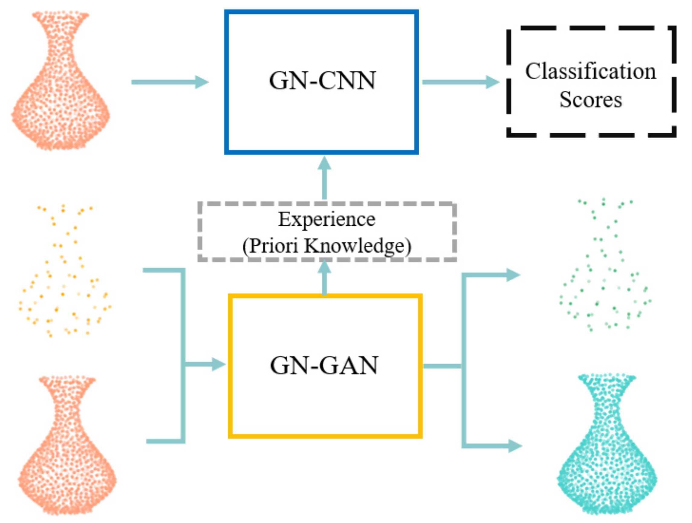
As shown in Figure 1, we pre-trained the GN-GAN to a warm start [5,6] GN-CNN, which is the 3D point cloud analysis network. GN-GAN obtains the global point cloud feature (experience) vector. Then the vector is plugged in as prior knowledge into the backbone network of GNConv, which is used as the convolution-like operation in GN-CNN. Using the original and downsampled input helps to learn multi-scale point cloud features.
Furthermore, the 3D models in the Metaverse are usually acquired with a focus on the model’s visual appearances instead of the exact point positions, for example, for driving [7] and indoor navigation [8], more attention is usually paid to the model’s appearance to make sure the models look good, instead of the model actual accuracy, which is usually the focus of computer-aided design (CAD). Based on this, unlike existing (few-shot) learning methods [9,10], we propose unleashing the model appearance to further augment the information. The model’s local surface variance and normal information determine how light is reflected, and how the model’s appearance is perceived by the viewers. Therefore, they are utilized in the proposed pipeline: First, in the encoder of the encoder/decoder framework of the GN-GAN generator, we introduced a graph convolution-enhanced combined multilayer perceptron operation (CMLP [11]), namely GCMLP, by adding several graph convolution layers. Second, in GN-CNN, we utilize local neighborhood normal information.
Different from the existing graph convolution-based methods, such as DGCNN [12] and GeoConv [13], we used graph convolution to enhance CMLP [11], which does not handle geometric relationships well. By integrating the capability of CMLP in learning different levels of feature information and the capability of graph convolution in learning local spatial connection relationships, the local surface variance information can be better learned. Together with the normal information, the appearance of the model can be better captured.
In this paper, we focus on classification and few-shot learning (GN-CNN) as well as reconstruction (GU-GAN) tasks of 3D point cloud analysis. Our contributions are summarized as the following:
(1)
We propose a convolution neural network framework GN-CNN that is suitable for Metaverse applications. We propose a few-shot learning approach using an unsupervised generative adversarial network GU-GAN to warm start GN-CNN by generating prior knowledge.
(2)
We propose the graph-enhanced combined multilayer perceptron operation (GCMLP) in the GN-GAN encoder and normal-aware graph convolution operation GNConv to better capture the model appearance information.
(3)
Based on evaluations, state-of-the-art 3D point cloud classification accuracy and few-shot learning accuracy on ModelNet40 and ModelNet10 are achieved.
Please refer to the table of abbreviations for the main abbreviations used in this paper.

2. Related Work

2.1. Deep Learning on 3D Point Cloud Analysis

Unlike the 2D image, the 3D point cloud does not have a straightforward regular grid (pixels), so it cannot use CNN directly. Therefore, some early work converts point clouds to other regularized representations, such as volumetric 2D views [14,15,16,17,18,19] or representations [20,21,22,23,24]. Although voxelization-based methods and view-based methods can achieve good results on point cloud analysis tasks, the resolution of voxel grids always seriously affects the efficiency of the neural network, and view-based methods always consume much time in data preparation. PointNet [1] and PointNet++ [25] first use the 3D coordinates of the point as direct input. Some works [26,27,28,29] also input point clouds directly and construct their own networks based on PointNet [1] and PointNet++ [25]. However, they extract features on each point independently, which cannot easily learn geometric relationships among points of the point cloud.

2.2. Graph-Based Works on Point Cloud Analysis

As a milestone in the use of graph convolution on 3D point clouds, DGCNN [12], dubbed EdgeConv, uses the k-nearest neighbor algorithm (k-NN) to construct a local neighborhood graph and update the graph structure on deeper latent layers. With the stacking of EdgeConv, DGCNN can learn the global features of the 3D point cloud. However, EdgeConv ignores the directional information of the edges formed by the local neighborhood. RSCNN [30] learns the weight matrix by constructing a local neighborhood graph and then multiplies it with the features in the network. GeoConv [13] builds a graph structure and decomposes the edge features in latent layers according to the orthogonal basis. GeoConv uses the directional information to enrich the geometric properties in the graph convolution and achieved better results than EdgeConv. However, GeoConv still only pays attention to the spatial connection relationship between neighboring points when constructing the graph. Therefore, the obtained directional information involves the spatial relationship between the points, the local surface information in different levels (i.e., low and high levels), and normal information are not addressed.

2.3. Point Cloud Reconstruction and Completion Based on Deep Learning

Some works use GAN-based methods on point cloud reconstruction and completion. The L-GAN [31] is the first to use deep learning methods for point cloud completion in the 3D field, but since L-GAN does not focus on the point cloud completion task, the results are not ideal. Some point cloud completion works pay more attention to real-time performances, such as RL-GAN-Net [2], but the accuracy is not high. Some other works plug graph convolution into the GAN-based networks. Valsesia et al. [32] used graph convolution for unsupervised point cloud reconstruction, defining the graph as the output of the generator. Huang et al. [11] further studied 3D point cloud completion and proposed PF-Net based on unsupervised learning, using the pyramid structure to construct the decoder. PF-Net obtains high-precision 3D point cloud completion results by jointly training both the generator and discriminator.

2.4. Summary

Please refer to Table 1 for a comparison with other methods.
Current few-shot learning methods [9,10,33] of 3D point clouds mostly learn semantic information from the support point sets and then generalize it to analyze the query point sets. Different from the existing methods, we use a GAN-based and appearance-aware approach. Our methods can improve the accuracy of results compared to the voxel-based and non-graph-based methods; please refer to the results section.

3. Method

This section presents the proposed GN-CNN and GN-GAN and the core operations in the two networks. We will first introduce our overall architecture, GN-CNN, and warm start strategy, then describe the structure of GCMLP and GN-GAN.

3.1. The Overall Architecture and GN-CNN

The overall network architecture includes GN-CNN, which is the backbone network for point cloud classification and few-shot learning tasks, as well as GN-GAN, which aims at warm starting GN-CNN. GN-GAN can also be used for point cloud reconstruction tasks.
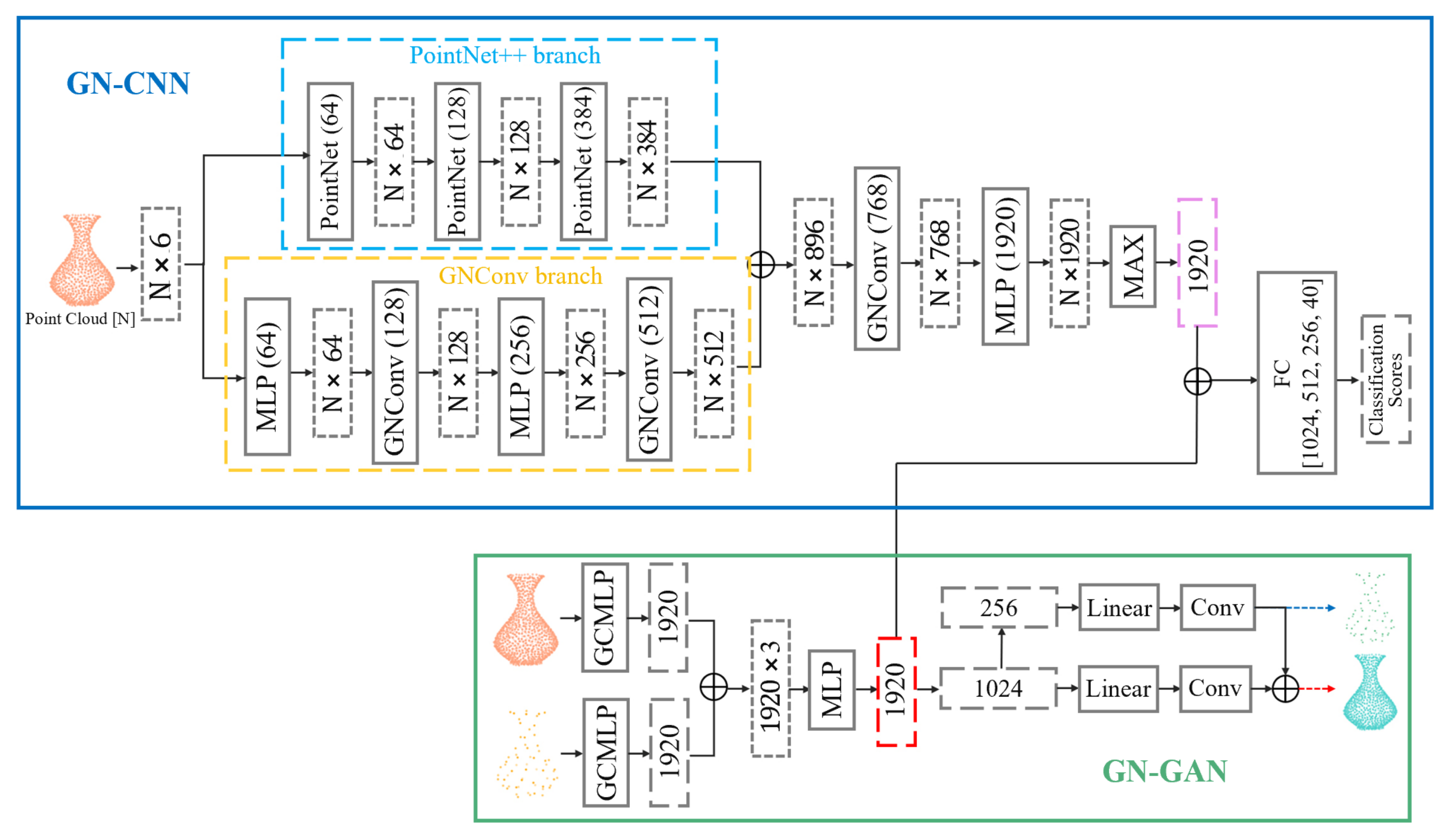
Our GN-CNN pipeline is inspired by Geo-CNN [11], and the network structure is also divided into two branches, as shown in Figure 2. The first branch of GN-CNN is PointNet++, using PointNet to extract features layer by layer. Each layer uses multilayer perceptron (MLP) and max pooling to abstract features to high dimensions, and the three layers of PointNet encode features into dimensions [64, 128, 384], and finally, we obtain a feature size of N × 384 , where N is the number of points.
In the second branch of GN-CNN, the input is the same as the first branch. First, the input point cloud feature with a size of N × 6 into an MLP to map the size of the feature to N × 64 , and then pass a layer of GNConv to obtain the feature with a size of N × 128 , and then pass an MLP to obtain the feature with a size of N × 256 and follow a layer of GNConv to obtain the feature with a size of N × 512 . The N × 384 feature obtained by the first branch is connected to obtain a feature of size N × 896 , and then input into a layer of GNConv to obtain a feature of size N × 768 , and finally passes through an MLP to obtain a feature of size N × 1920 . Next, we use max pooling to obtain a vector with length [1920]. The vector with length [1920] is the point cloud global feature representation vector.
Next, we use the prior knowledge extracted by the GN-GAN encoder with the same length of [1920] for feature aggregation with the point cloud global feature vector extracted by GN-CNN encoder, and GN-CNN is warm-started. The aggregation function adopts an element-wise sum. The GN-CNN decoder consists of four FC layers with the vectors of output lengths [1024, 512, 256, C], where C is the number of classes in the point cloud classification tasks.
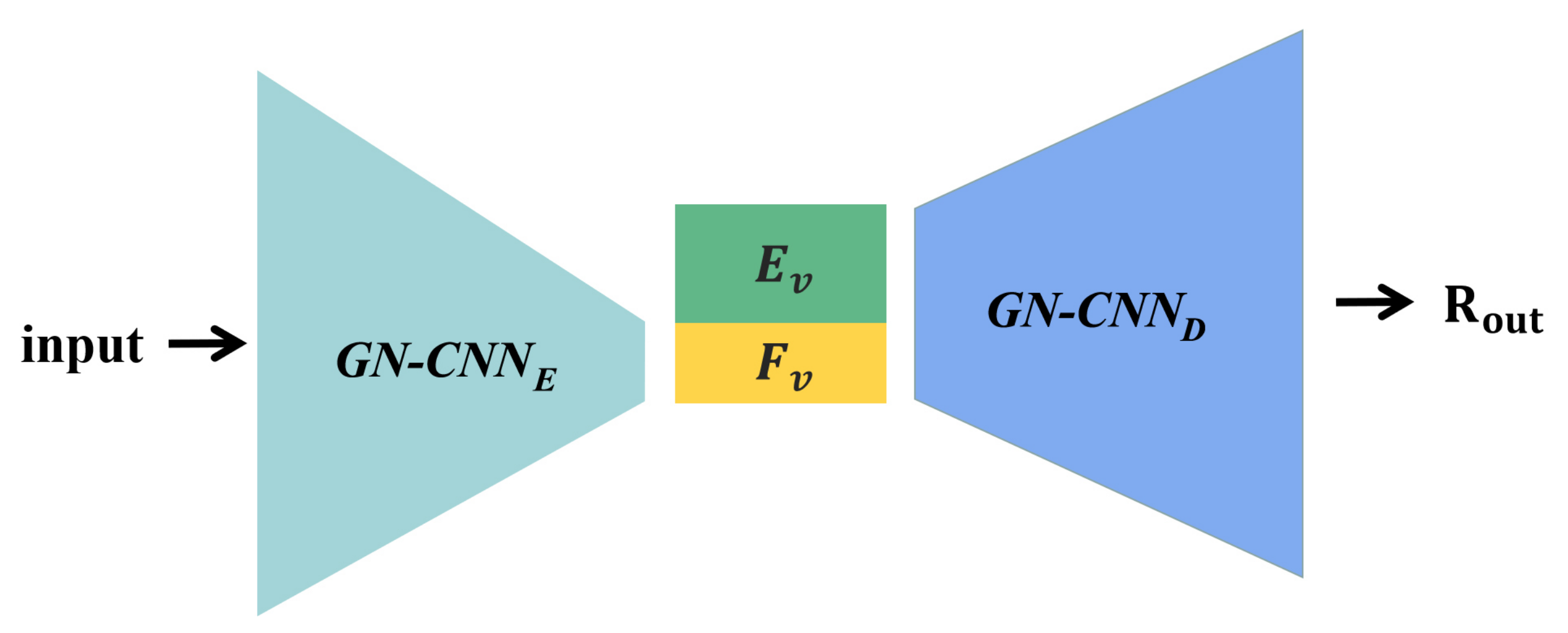
3.2. Warm Start

The warm start techniques are often used in the field of deep learning [5,6,34] and reinforcement learning. The warm start is to initialize the network parameters to make networks have a particular experience at the beginning of training. This method can accelerate the convergence of the neural network. When the data size is limited, the neural network can make corresponding judgments based on the experience knowledge to obtain better few-shot learning results. Our warm start strategy is shown in Figure 3. G N C N N E is the encoder of GN-CNN, G N C N N D is the decoder of GN-CNN, F v is the global feature representation extracted by the GN-CNN encoder, and E v is the experience knowledge. We aggregate E v and F v , and then input them into the decoder of GN-CNN. R o u t is the output of the GN-CNN decoder. The output R o u t of the GN-CNN decoder is defined as:
R o u t = G N C N N D ( A ( F v , E v ) ) = G N C N N D ( A ( G N C N N E ( P ) , G N E ( P ) ) ) ,
where G N E ( ) represents the encoder of GN-GAN, P is a point cloud, A ( ) is the aggregation function, we use element-wise add as the aggregation function.
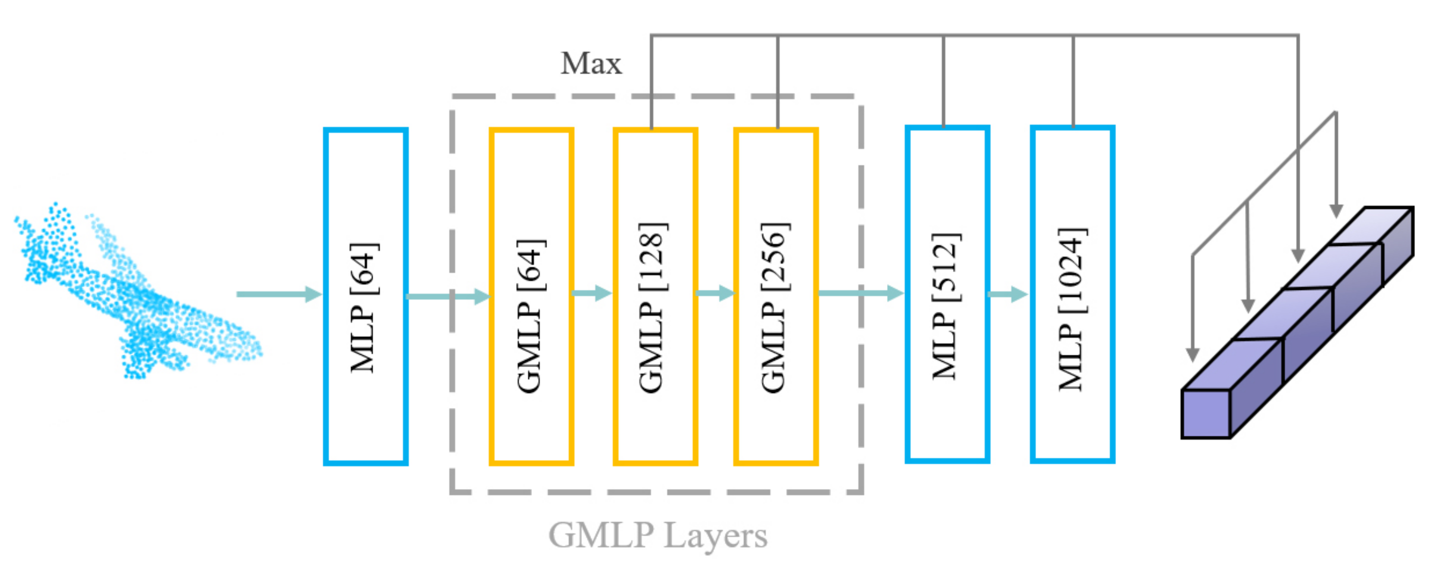
3.3. GCMLP

CMLP [11] takes the maximum value in each channel on low-level and high-level through MLP and then concatenates the vector after the max pooling. CMLP can integrate low-level and high-level features to learn multi-level information better, but it does not handle the geometric relationship information among points.
Since graph convolution can handle geometric relationships among points, especially for the local neighborhood learning of point clouds, we propose GCMLP, as shown in Figure 4, to improve CMLP performance by using a graph convolution layer named GMLP. In GCMLP, three MLP layers in CMLP are replaced with GMLP layers, while still concatenating the low-level and high-level feature vectors after max pooling. For a GMLP layer, we first use k-NN for each point p i ( i = 1 , 2 , , N ) within N points to find the k nearest neighbors p j ( j = 1 , 2 , , k ) and take k neighboring points p j as source points and p i as target points and construct an edge p j p i (including the self-loop from p i to p i ). Finally, we concatenate [ p j p i , p i ] , and then go through the MLP layer.
GCMLP first uses an MLP to encode the dimensions of the original point cloud to [64], then uses three GMLP layers to encode the dimensions to [64, 128, 256], and finally is followed by two MLP layers to encode the dimensions to [512, 1024]. We max pool the output of the last four layers and concatenate the four vectors. The lengths of the four vectors are [128, 256, 512, 1024].

3.4. GN-GAN and Loss Function

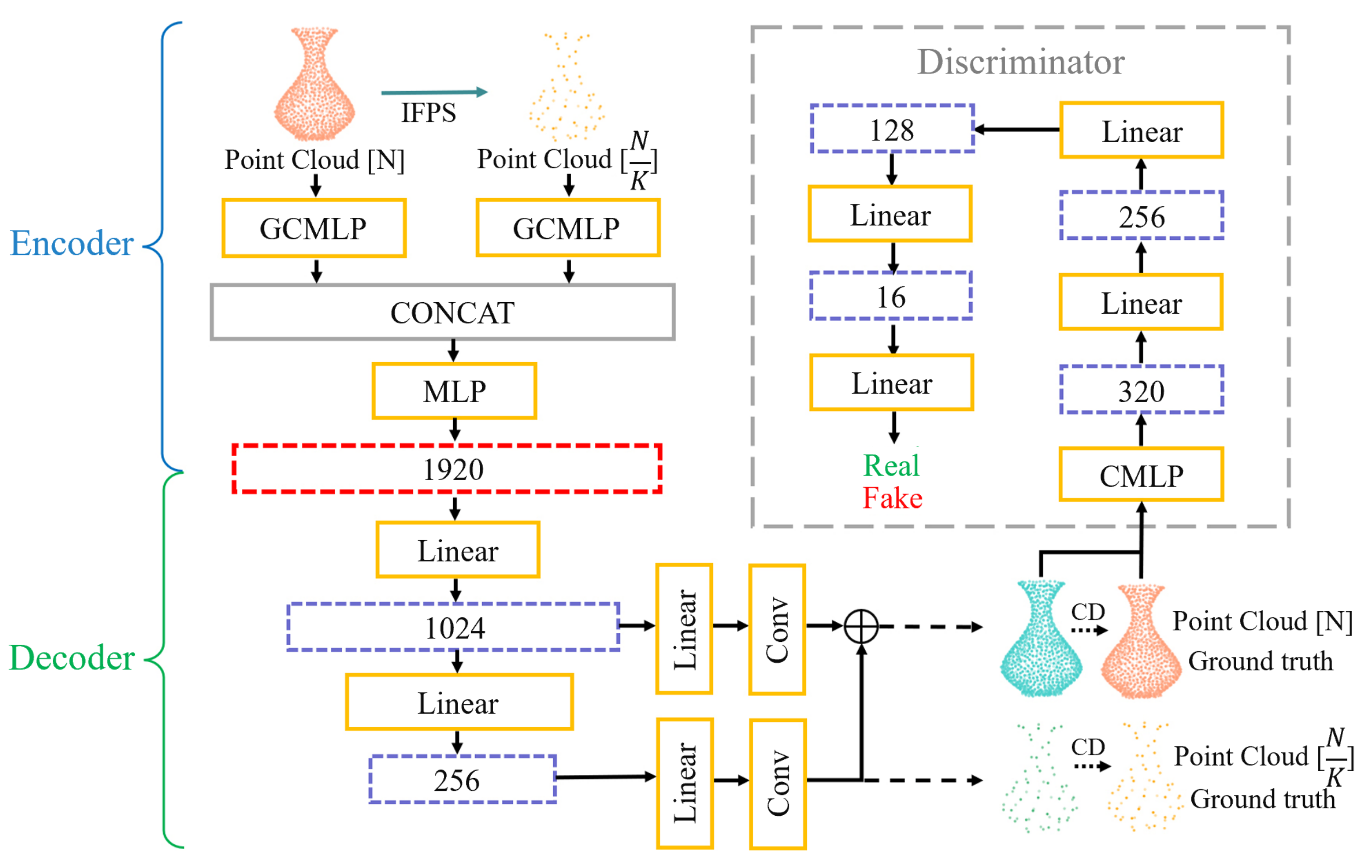
The overall structure of GN-GAN is shown in Figure 5. We use iterative farthest point sampling (IFPS) to downsample the input point cloud to obtain two resolutions of the point cloud. The encoder of the GN-GAN generator takes both two resolutions as input. The number of points in the high-resolution point cloud is N, and the number in the low-resolution point cloud after down-sampling is N 2 = N K . The point clouds with two resolutions are passed through two GCMLPs, respectively, and the generator reconstructs two point clouds with the same resolutions as respective inputs. We concatenate the two feature vectors obtained through GCMLP and input them into an MLP to encode the dimensions of the global feature vector F V to 1920. CD is the Chamfer distance to evaluate the difference between the reconstructed point cloud and ground truth.
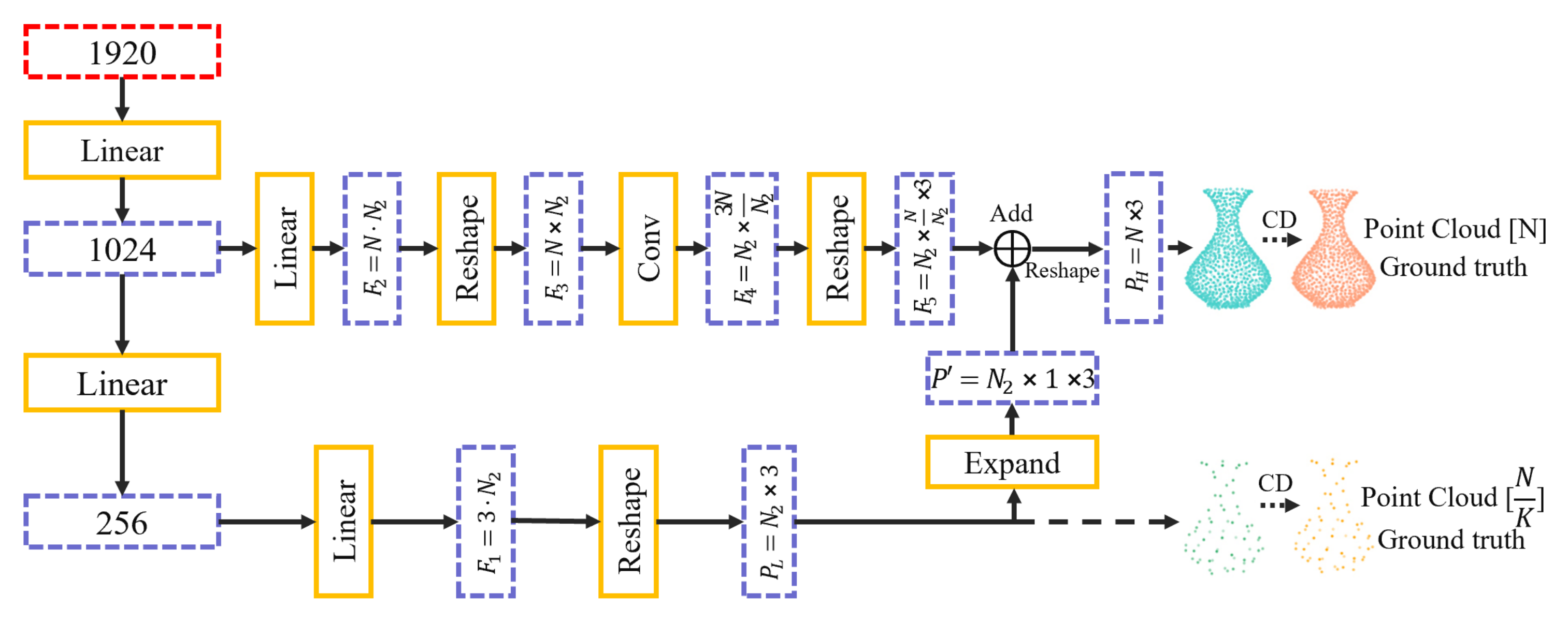
The structure of the decoder in the GN-GAN generator is shown in Figure 6, where F V is inputted into the decoder. The red box in Figure 6 is F V . We first use two fully connected (FC) layers to encode the dimensions of F V to [1024, 256]. The [256] vector is used to obtain the vector F 1 with the size of 3 · N 2 through an FC layer, and F 1 is reshaped to the size N 2 × 3 to obtain P L , which is the low-resolution reconstructed point cloud. Next, we use the [1024] vector to obtain F 2 which size is N · N 2 through the FC layer, reshape F 2 into F 3 of size N × N 2 , and input F 3 into a convolution layer to obtain F 4 of size N 2 × 3 N N 2 . We reshape F 4 to F 5 of size N 2 × N N 2 × 3 . At this point, we expand P L to N 2 × 1 × 3 , and add it to F 5 . Finally, we reshape it to obtain the high-resolution reconstructed point clouds P H of size N × 3 .
The reconstruction loss of GN-GAN is defined using the Chamfer distance. Chamfer distance is the average nearest squared distance between two point clouds. Define the ground truth point cloud as P r e a l = { p 1 , p 2 , , p N } , and the reconstructed point cloud is P f a k e = { p 1 , p 2 , , p N } , then Chamfer distance L C D between P f a k e and P r e a l is divided into two parts C D 1 and C D 2 :
C D 1 = 1 P r e a l i = 1 N min j [ 1 , N ] p i p j 2 2
C D 2 = 1 P f a k e j = 1 N min i [ 1 , N ] p i p j 2 2 .
Finally, L C D is defined as:
L C D = C D 1 + C D 2 .
The reconstruction loss of GN-GAN is defined as:
L g e n = L C D h + α L C D l ,
where L C D h is the Chamfer distance between the high-resolution reconstructed point cloud and the ground truth, and L C D l is the Chamfer distance between the low-resolution reconstructed point cloud and the corresponding ground truth, and α is a hyperparameter.
The structure of the discriminator is shown in Figure 5, and we divide the adversarial loss of the GN-GAN discriminator into two parts, which correspond to inputting the ground truth point cloud into the discriminator and inputting the reconstructed point cloud into the discriminator, respectively. The generator mapping process is defined as G ( · ) and the discriminator mapping process is defined as D ( · ) , then the adversarial loss is defined as:
L a d v = 1 i N l o g ( D ( x i ) ) + 1 i N l o g ( D ( G ( x i ) ) ) ,
where x i X , i 1 , 2 , , N . The joint loss of GN-GAN is defined as:
L = λ g e n L g e n + λ a d v L a d v ,
where λ g e n and λ a d v are weights to balance two parts of joint loss, which satisfy:
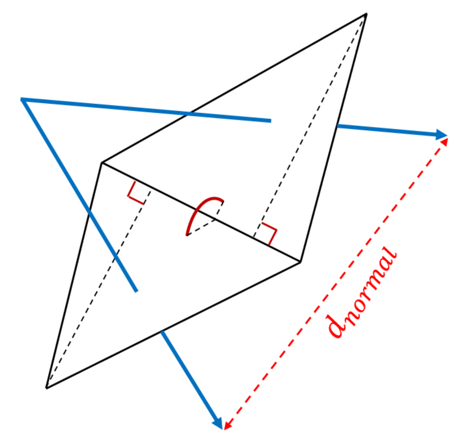
λ g e n + λ a d v = 1 .

3.5. GNConv

GNConv is designed to capture the visual variance of the local surface formed by the point cloud and augment the information with it. Since the normal of a point can depict the information and appearance of the local neighborhood, so we use normals. As shown in Figure 7, d n o r m a l represents the distance between the two normals, reflecting the visual variance of the surface. Conceptually, when d n o r m a l is large, the local surface appearances vary violently, which means there are more features (important information).
Inspired by GeoConv [13], GNConv includes the distance of normals between the center point and the neighboring points on the local neighborhood graph in each iteration. Define the point cloud as P = { p 1 , p 2 , . . . , p N } , where p i = { x i , y i , z i } . Taking each point of P as the center point, take the spherical neighborhood S ( p i ) = { p j | p i p j r } with radius r, and the normal set is N P = { n p 1 , n p 2 , , n p N } . As the iteration progresses, gradually increase r to obtain a larger receptive field. Define X p i l R C as the feature of p i obtained after the lth iteration of GNConv, then the definition of GNConv is as follows:
X p i l = W c X p i l 1 + W e p j S ( p i ) f d ( p i , p j , r ) f n ( p i , p j ) f d ( p i , p j , r ) .
As shown in Equation (9), the feature of p i on the lth layer has two parts. The first part is the output of the previous layer X p i l 1 multiplied by the center point weight W c to extract the center point feature, and the second part is the edge property between the center point and neighboring points in the spherical neighborhood. The corresponding feature is multiplied by the weight W e and W e to enlarge the feature dimension to be the same as the dimension of the first part. In the second part, f n ( p i , p j ) is defined as:
f n ( p i , p j ) = W n n ( p i , p j ) + b c o s 2 ( θ b ) W b X e i j l 1 .
Before each iteration, we take each point p i as the center of the local spherical neighborhood and determine the neighborhood S ( p i ) with a radius of r. The normal edge feature n ( p i , p j ) between the center point and the neighboring points in the spherical neighborhood is defined as:
n ( p i , p j ) = n p j n p i ,
where p j S ( p j ) , W n is the weight of normal edge features. The edge feature X e i j l 1 is defined as:
X e i j l 1 = X p j l 1 X p i l 1 .
For each spherical neighborhood, we construct an orthogonal basis with p i as the origin and decompose the edge features along with the orthogonal basis, and c o s ( θ b ) is the cosine between each component and the corresponding orthogonal basis. W b is the weight for feature extraction of the components along with three orthogonal bases. After the feature components of the three edges are mapped to the high-dimensional feature space, we aggregate the components by c o s ( θ b ) . Finally, we aggregate the edge feature X e i j l 1 and the normal edge feature n ( p i , p j ) as shown in Equation (10).
In Equation (9), f d ( p i , p j , r ) is the weight function, and the weight is dynamically changed according to the distance between p j and p i , which is defined as:
f d ( p i , p j , r ) = ( r p i p j ) 2 .

4. Experiments

4.1. Implementation Details

In our experiments, the GPU used in the classification experiment and the ablation experiment was NVIDIA GeForce GTX 2080ti; the GPU used in the few-shot learning experiment and the visualization of GN-GAN reconstruction results was NVIDIA GeForce GTX 1070.
In the 3D point cloud classification experiment and the few-shot learning experiment, the input 3D point cloud of GN-CNN contained 1024 points. The radii for three GNConv layers were 0.15, 0.3, and 0.6. The first branch and the second branch both used the Adam optimizer and the cosine annealing strategy. The training batch_size was 10, and the test batch_size was 8.
When pre-training GN-GAN, the input point cloud resolution was 1024 points and 64 points after IFPS downsampling with K = 16. The generator used the Adam optimizer and StepLR to update the parameters every 40 epochs. The discriminator also used the Adam optimizer and StepLR to update the parameters every 40 epochs. The training batch_size was 16, and the test batch_size was 8.

4.2. Dataset

Our experiments used ModelNet40 [20] and ModelNet10 [20]. For classification, we carried out experiments on both ModelNet10 and ModelNet40. The input point cloud resolution was 1024 points, and we used all samples from the training and test sets. For few-shot learning, we used ModelNet40 and randomly reduced 50%, 70%, 90%, and 95% of the total number of training samples; that is, using 50%, 30%, 10%, and 5% of the total number of training samples. We kept the number of testing samples unchanged, so the few-shot learning experiment used five training set sizes, including the original training set. We used ModelNet40 to pre-train GN-GAN for experience knowledge.

4.3. Classification

We used warm-start GN-CNN to perform classification experiments on ModelNet40 and ModelNet10. The experiment’s results are shown in Table 2 and Table 3, where MA is the mean per-class accuracy and OA is the overall accuracy.
The results on ModelNet40 are shown in Table 2. Using our method, MA is 90.5% and OA is 93.0%; OA increased by 3.8% compared with PointNet [1], and 2.3% compared with PointNet++ [25]. Through a warm start strategy, the OA of our method increased by 0.1% compared to the milestone work DGCNN [12] in the field of graph convolution. Note that our result did not reach the reported OA of 93.4% in the original Geo-CNN [13] when training 200 epochs using the same network structure and parameter settings, but it is slightly better than the OA of the reproduced Geo-CNN, which is 92.9% (the same as DGCNN). In our opinion, there are two main reasons: first, the reproduction process is different from the original paper, which causes a different training result, and second, the hardware and the number of epochs are different. Using more epochs, similar results as in the original paper should be achieved.
The OA of our method on ModelNet10 can reach 95.9%. As shown in Table 3, the OA increased by 12.4% compared with 3DShapeNets [20], and increased by 1.5% compared with KCNet. Compared with some work proposed in recent years, such as LP-3DCNN, 3DCapsule, VIPGAN, Point2Sequence, and MHBN, our result on ModelNet10 is the best. Moreover, on the official website of Princeton ModelNet, the overall accuracy ranking of the work performed on ModelNet10 for classification tasks is provided as the ModelNet benchmark leaderboard, and the performance of GN-CNN is ranked fifth.

4.4. Few-Shot Learning

Our few-shot learning experiment uses ModelNet40 and the results are shown in Table 4. Moreover, 100%, 50%, 30%, 10%, and 5% represent the five training set sizes after random sampling. Since the other four methods did not conduct few-shot learning, we used the other four methods to perform few-shot learning under the same conditions as the GN-CNN experimental environment.
We can see from Table 4 that our GN-CNN on the original training set can achieve similar results as DGCNN and Geo-CNN, but after the size of the training set is reduced, the OA and MA of GN-CNN are better than Geo-CNN. When the training set size reduces to 30%, the OA of GN-CNN classification increases by 2.5% compared with Geo-CNN, and the MA increases by 3.1%. Moreover, since the number of samples in the ModelNet40 training set is 9843, and the number of samples in the test set is 2468, there are only about 500 samples in the training set when we reduce the size to 5% of the original training set, and the number of training samples only accounts for about 20% of the number of samples in the test set. In this case, compared with DGCNN, the OA of GN-CNN increased by 3.3%, and the MA increased by 4.6%.

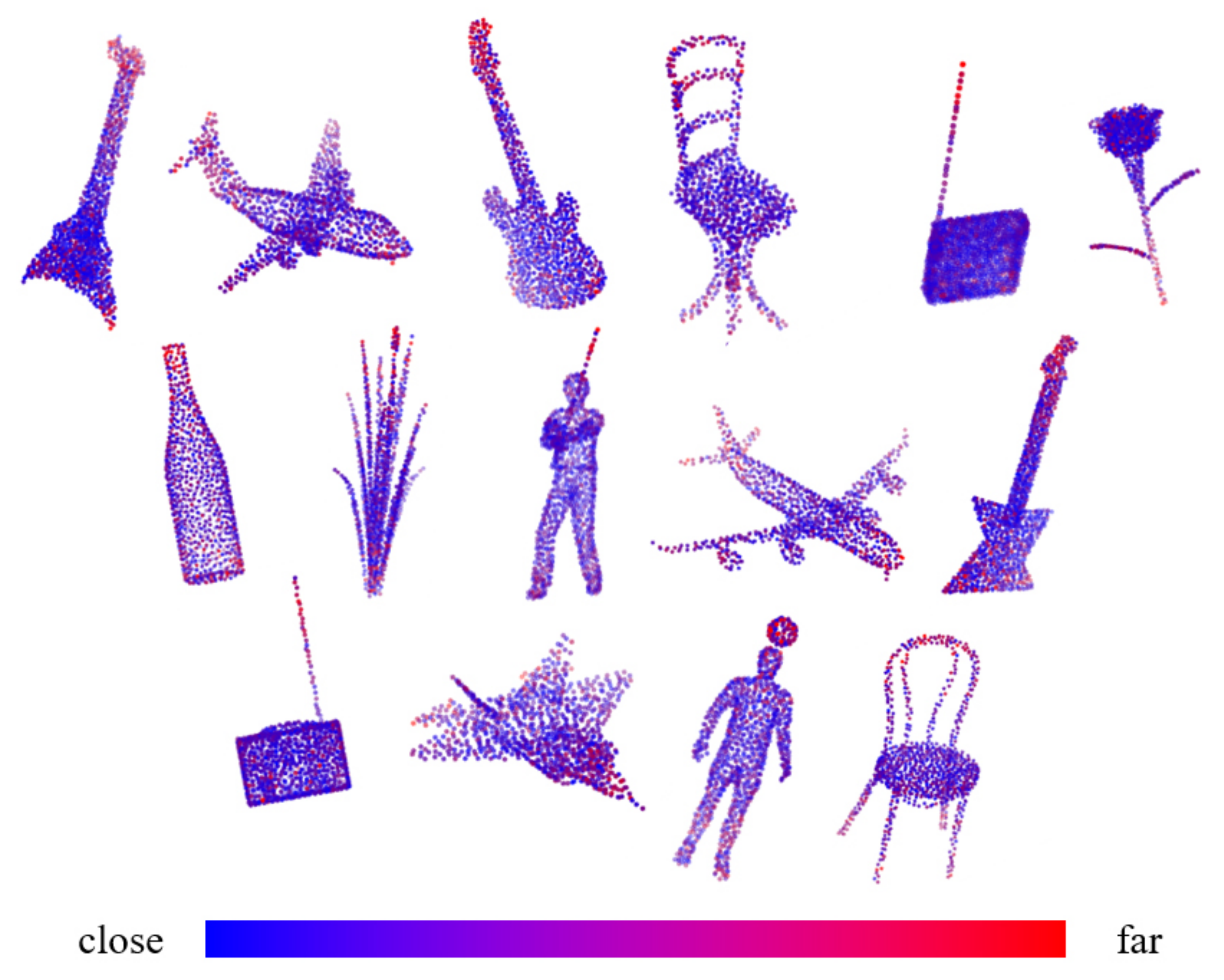
4.5. Reconstruction Results of GN-GAN

To justify the prior knowledge extracted by the GN-GAN containing useful point cloud information, we compare the point cloud reconstructed by the decoder with the ground truth. We use the heatmap to visualize the comparison results, as shown in Figure 8. When the point is closer to blue, the difference between the reconstructed and real points is smaller.
As shown in Figure 8, although the reconstructed points deviate from the real points in areas with more details of the 3D point clouds, such as the tips of airplane wings, the neck of bottles, and the plant leaves, GN-GAN can reconstruct point clouds that are very close to the ground truth on the whole, which shows that the prior knowledge extracted by the encoder in the GN-GAN generator is helpful.

4.6. Ablation Study

The ablation study was conducted using ModelNet40. The training set size was 5% of the original. The results are shown in Table 5. Since our GN-CNN and GNConv are inspired by Geo-CNN and GeoConv, the Geo-CNN is chosen as the “Baseline”. To compare the performance of GNConv and GeoConv, in “Baseline (GNConv)”, the GeoConv is replaced with GNConv. Compared with “Baseline”, GN-CNN not only uses GNConv to extract features but also includes prior knowledge from the GN-GAN generator. The encoder of the generator in GN-GAN relies on GCMLP to extract features. To compare the performance of GCMLP and CMLP, in “Baseline (GNConv) + CMLP”, the GCMLP of GN-GAN is replaced with CMLP, and the prior knowledge extracted by CMLP is plugged into “Baseline (GNConv)”. In “Baseline + GCMLP”, the prior knowledge obtained through GN-GAN is plugged into Geo-CNN.
Comparing the OA of “Baseline” and “Baseline (GNConv)”, it is shown that GNConv has a stronger extracting ability than GeoConv. Comparing “Baseline (GNConv)” and “Baseline (GNConv) + CMLP”, as well as “Baseline” and “Baseline + GCMLP”, it is shown that prior knowledge helps improve the accuracy of few-shot learning. Comparing “Baseline (GNConv) + CMLP” and our GN-CNN, it is shown that GCMLP has a stronger feature-extracting ability than CMLP.
To further compare the performance of GCMLP and CMLP, two layers of GCMLP in GN-GAN are replaced with CMLP and named GN-GAN (CMLP). As shown in Table 6, we use ground truth and predicted (GT-pred) error to evaluate the performance. GT-pred error computes the average squared distance from each point in the ground truth to its closest in the reconstructed point cloud. We observed that when using GCMLP to extract features, the result is smaller, which means that the reconstruction result of GN-GAN is better than that of GN-GAN (CMLP). This indicts that GCMLP has a stronger feature-extracting ability.

5. Conclusions

In this paper, we propose a convolutional neural network framework GN-CNN with normal-aware convolution operation GNConv, which is suitable for Metaverse applications. To solve the problem of few-shot learning of point clouds, we propose an unsupervised generative adversarial network GN-GAN, based on graph convolution-enhanced multilayer perceptron operation GCMLP for point cloud reconstruction (for extracting experience knowledge to warm start GN-CNN). The performance was evaluated on ModelNet40 and ModelNet10.
It is still challenging to reconstruct all local detailed features and the accuracy still has room to improve. In the future, we plan to study more geometric characteristics of the point cloud to improve the feature extraction performance and explore more prior knowledge of point cloud geometric information to promote the learning of the backbone network.

Author Contributions

Conceptualization, Q.S. and Y.S.; methodology, Q.S., Y.X. and C.Y.; software, Q.S. and Y.X.; validation, C.Y.; investigation, Q.S., Y.X. and Y.S.; writing—original draft preparation, Q.S., Y.X., Y.S., J.S.A.L. and K.C.; writing—review and editing, J.S.A.L. and K.C.; supervision, Y.S. and K.C. All authors have read and agreed to the published version of the manuscript.

Funding

This research was funded by The Startup Foundation for Introducing Talent of NUIST grant number 2022r075, National Natural Science Foundation of China grant number U22B2002 and Natural Science Foundation of Jiangsu Province grant number BK20191329.

Institutional Review Board Statement

Not applicable.

Informed Consent Statement

Not applicable.

Data Availability Statement

3rd Party Data.

Conflicts of Interest

The authors declare no conflict of interest.

Abbreviations

The following abbreviations are used in this manuscript:
AbbreviationExplanation
CNNconvolutional neural network
(C)MLP(combined) multilayer perceptron
GANgenerative adversarial network
Convconvolution
FCfully connected
CDChamfer distance
IFPSiterative farthest point sampling
MAmean per-class accuracy
OAoverall accuracy

References

  1. Qi, C.; Su, H.; Kaichun, M.; Guibas, L.J. PointNet: Deep Learning on Point Sets for 3D Classification and Segmentation. In Proceedings of the 2017 IEEE Conference on Computer Vision and Pattern Recognition (CVPR), Honolulu, HI, USA, 21–26 July 2017; pp. 77–85. [Google Scholar] [CrossRef]
  2. Sarmad, M.; Lee, H.J.; Kim, Y.M. RL-GAN-Net: A Reinforcement Learning Agent Controlled GAN Network for Real-Time Point Cloud Shape Completion. In Proceedings of the 2019 IEEE/CVF Conference on Computer Vision and Pattern Recognition (CVPR), Long Beach, CA, USA, 15–20 June 2019; pp. 5891–5900. [Google Scholar] [CrossRef]
  3. He, C.; Zeng, H.; Huang, J.; Hua, X.S.; Zhang, L. Structure Aware Single-Stage 3D Object Detection From Point Cloud. In Proceedings of the 2020 IEEE/CVF Conference on Computer Vision and Pattern Recognition (CVPR), Seattle, WA, USA, 13–19 June 2020; pp. 11870–11879. [Google Scholar] [CrossRef]
  4. Shi, W.; Rajkumar, R. Point-GNN: Graph Neural Network for 3D Object Detection in a Point Cloud. In Proceedings of the 2020 IEEE/CVF Conference on Computer Vision and Pattern Recognition (CVPR), Seattle, WA, USA, 13–19 June 2020; pp. 1708–1716. [Google Scholar] [CrossRef]
  5. Garcez, A.S.D.; Broda, K.B.; Gabbay, D.M. Neural-Symbolic Learning Systems. In Neural-Symbolic Cognitive Reasoning; Springer: Berlin/Heidelberg, Germany, 2009; pp. 35–54. [Google Scholar] [CrossRef]
  6. Hu, Z.; Ma, X.; Liu, Z.; Hovy, E.; Xing, E. Harnessing Deep Neural Networks with Logic Rules. In Proceedings of the 54th Annual Meeting of the Association for Computational Linguistics, Berlin, Germany, 7–12 August 2016. [Google Scholar]
  7. Chen, X.; Ma, H.; Wan, J.; Li, B.; Xia, T. Multi-view 3D Object Detection Network for Autonomous Driving. In Proceedings of the 2017 IEEE Conference on Computer Vision and Pattern Recognition (CVPR), Honolulu, HI, USA, 21–26 July 2017; pp. 6526–6534. [Google Scholar] [CrossRef]
  8. Zhu, Y.; Mottaghi, R.; Kolve, E.; Lim, J.J.; Gupta, A.; Fei-Fei, L.; Farhadi, A. Target-driven visual navigation in indoor scenes using deep reinforcement learning. In Proceedings of the 2017 IEEE International Conference on Robotics and Automation (ICRA), Singapore, 29 May–3 June 2017; pp. 3357–3364. [Google Scholar] [CrossRef]
  9. Zhao, N.; Chua, T.S.; Lee, G.H. Few-shot 3d point cloud semantic segmentation. In Proceedings of the IEEE/CVF Conference on Computer Vision and Pattern Recognition, Nashville, TN, USA, 20–25 June 2021; pp. 8873–8882. [Google Scholar]
  10. Kang, D.; Cho, M. Integrative Few-Shot Learning for Classification and Segmentation. In Proceedings of the IEEE/CVF Conference on Computer Vision and Pattern Recognition, New Orleans, LA, USA, 18–24 June 2022; pp. 9979–9990. [Google Scholar]
  11. Huang, Z.; Yu, Y.; Xu, J.; Ni, F.; Le, X. PF-Net: Point Fractal Network for 3D Point Cloud Completion. In Proceedings of the 2020 IEEE/CVF Conference on Computer Vision and Pattern Recognition (CVPR), Seattle, WA, USA, 13–19 June 2020; pp. 7659–7667. [Google Scholar] [CrossRef]
  12. Wang, Y.; Sun, Y.; Liu, Z.; Sarma, S.E.; Bronstein, M.M.; Solomon, J.M. Dynamic Graph CNN for Learning on Point Clouds. ACM Trans. Graph. 2019, 38, 1–12. [Google Scholar] [CrossRef]
  13. Lan, S.; Yu, R.; Yu, G.; Davis, L.S. Modeling Local Geometric Structure of 3D Point Clouds Using Geo-CNN. In Proceedings of the 2019 IEEE/CVF Conference on Computer Vision and Pattern Recognition (CVPR), Long Beach, CA, USA, 15–20 June 2019; pp. 998–1008. [Google Scholar] [CrossRef]
  14. Su, H.; Maji, S.; Kalogerakis, E.; Learned-Miller, E. Multi-view Convolutional Neural Networks for 3D Shape Recognition. In Proceedings of the 2015 IEEE International Conference on Computer Vision (ICCV), Santiago, Chile, 7–13 December 2015; pp. 945–953. [Google Scholar] [CrossRef]
  15. Yang, Z.; Wang, L. Learning Relationships for Multi-View 3D Object Recognition. In Proceedings of the 2019 IEEE/CVF International Conference on Computer Vision (ICCV), Seoul, Republic of Korea, 27 October–2 November 2019; pp. 7504–7513. [Google Scholar] [CrossRef]
  16. Wei, X.; Yu, R.; Sun, J. View-GCN: View-Based Graph Convolutional Network for 3D Shape Analysis. In Proceedings of the 2020 IEEE/CVF Conference on Computer Vision and Pattern Recognition (CVPR), Seattle, WA, USA, 13–19 June 2020; pp. 1847–1856. [Google Scholar] [CrossRef]
  17. Lawin, F.J.; Danelljan, M.; Tosteberg, P.; Bhat, G.; Khan, F.S.; Felsberg, M. Deep Projective 3D Semantic Segmentation. In Proceedings of the International Conference on Computer Analysis of Images and Patterns, Ystad, Sweden, 22–24 August 2017; Felsberg, M., Heyden, A., Krüger, N., Eds.; Springer International Publishing: Cham, Switzerland, 2017; pp. 95–107. [Google Scholar]
  18. Feng, Y.; Zhang, Z.; Zhao, X.; Ji, R.; Gao, Y. GVCNN: Group-View Convolutional Neural Networks for 3D Shape Recognition. In Proceedings of the 2018 IEEE/CVF Conference on Computer Vision and Pattern Recognition, Salt Lake City, UT, USA, 18–22 June 2018; pp. 264–272. [Google Scholar] [CrossRef]
  19. Yu, T.; Meng, J.; Yuan, J. Multi-view Harmonized Bilinear Network for 3D Object Recognition. In Proceedings of the 2018 IEEE/CVF Conference on Computer Vision and Pattern Recognition, Salt Lake City, UT, USA, 18–22 June 2018; pp. 186–194. [Google Scholar] [CrossRef]
  20. Wu, Z.; Song, S.; Khosla, A.; Yu, F.; Zhang, L.; Tang, X.; Xiao, J. 3D ShapeNets: A deep representation for volumetric shapes. In Proceedings of the 2015 IEEE Conference on Computer Vision and Pattern Recognition (CVPR), Boston, MA, USA, 7–12 June 2015; pp. 1912–1920. [Google Scholar] [CrossRef]
  21. Maturana, D.; Scherer, S. VoxNet: A 3D Convolutional Neural Network for real-time object recognition. In Proceedings of the 2015 IEEE/RSJ International Conference on Intelligent Robots and Systems (IROS), Hamburg, Germany, 28 September–3 October 2015; pp. 922–928. [Google Scholar] [CrossRef]
  22. Riegler, G.; Ulusoy, A.O.; Geiger, A. OctNet: Learning Deep 3D Representations at High Resolutions. In Proceedings of the 2017 IEEE Conference on Computer Vision and Pattern Recognition (CVPR), Honolulu, HI, USA, 21–26 July 2017; pp. 6620–6629. [Google Scholar] [CrossRef]
  23. Huang, J.; You, S. Point cloud labeling using 3D Convolutional Neural Network. In Proceedings of the 2016 23rd International Conference on Pattern Recognition (ICPR), Cancun, Mexico, 4–8 December 2016; pp. 2670–2675. [Google Scholar] [CrossRef]
  24. Rethage, D.; Wald, J.; Sturm, J.; Navab, N.; Tombari, F. Fully-Convolutional Point Networks for Large-Scale Point Clouds. In Proceedings of the Computer Vision—ECCV 2018, Munich, Germany, 8–14 September 2018; Ferrari, V., Hebert, M., Sminchisescu, C., Weiss, Y., Eds.; Springer International Publishing: Cham, Switzerland, 2018; pp. 625–640. [Google Scholar]
  25. Qi, C.R.; Yi, L.; Su, H.; Guibas, L.J. PointNet++: Deep Hierarchical Feature Learning on Point Sets in a Metric Space. In Proceedings of the 31st International Conference on Neural Information Processing Systems, Long Beach, CA, USA, 4–9 December 2017; Curran Associates Inc.: Red Hook, NY, USA, 2017; pp. 5105–5114. [Google Scholar]
  26. Aoki, Y.; Goforth, H.; Srivatsan, R.A.; Lucey, S. PointNetLK: Robust amp; Efficient Point Cloud Registration Using PointNet. In Proceedings of the 2019 IEEE/CVF Conference on Computer Vision and Pattern Recognition (CVPR), Long Beach, CA, USA, 15–20 June 2019; pp. 7156–7165. [Google Scholar] [CrossRef]
  27. Zhao, H.; Jiang, L.; Fu, C.W.; Jia, J. PointWeb: Enhancing Local Neighborhood Features for Point Cloud Processing. In Proceedings of the 2019 IEEE/CVF Conference on Computer Vision and Pattern Recognition (CVPR), Long Beach, CA, USA, 15–20 June 2019; pp. 5560–5568. [Google Scholar] [CrossRef]
  28. Lin, H.; Xiao, Z.; Tan, Y.; Chao, H.; Ding, S. Justlookup: One Millisecond Deep Feature Extraction for Point Clouds By Lookup Tables. In Proceedings of the 2019 IEEE International Conference on Multimedia and Expo (ICME), Shanghai, China, 8–12 July 2019; pp. 326–331. [Google Scholar] [CrossRef]
  29. Sun, X.; Lian, Z.; Xiao, J. SRINet: Learning Strictly Rotation-Invariant Representations for Point Cloud Classification and Segmentation. In Proceedings of the 27th ACM International Conference on Multimedia, Nice, France, 21–25 October 2019; Association for Computing Machinery: New York, NY, USA, 2019; pp. 980–988. [Google Scholar] [CrossRef]
  30. Liu, Y.; Fan, B.; Xiang, S.; Pan, C. Relation-Shape Convolutional Neural Network for Point Cloud Analysis. In Proceedings of the 2019 IEEE/CVF Conference on Computer Vision and Pattern Recognition (CVPR), Long Beach, CA, USA, 15–20 June 2019; pp. 8887–8896. [Google Scholar] [CrossRef]
  31. Achlioptas, P.; Diamanti, O.; Mitliagkas, I.; Guibas, L. Learning Representations and Generative Models for 3D Point Clouds. In Proceedings of the International Conference on Machine Learning, Stockholm, Sweden, 10–15 July 2018. [Google Scholar]
  32. Valsesia, D.; Fracastoro, G.; Magli, E. Learning Localized Generative Models for 3D Point Clouds via Graph Convolution. In Proceedings of the ICLR 2019, New Orleans, LA, USA, 6–9 May 2019. [Google Scholar]
  33. Dong, N.; Xing, E.P. Few-shot semantic segmentation with prototype learning. In Proceedings of the BMVC, Newcastle, UK, 3–6 September 2018; Volume 3. [Google Scholar]
  34. Kontschieder, P.; Fiterau, M.; Criminisi, A.; Bulò, S.R. Deep Neural Decision Forests. In Proceedings of the 2015 IEEE International Conference on Computer Vision (ICCV), Santiago, Chile, 7–13 December 2015; pp. 1467–1475. [Google Scholar] [CrossRef]
  35. Zaheer, M.; Kottur, S.; Ravanbhakhsh, S.; Póczos, B.; Salakhutdinov, R.; Smola, A.J. Deep Sets. In Proceedings of the 31st International Conference on Neural Information Processing Systems, Long Beach, CA, USA, 4–9 December 2017; Curran Associates Inc.: Red Hook, NY, USA, 2017; pp. 3394–3404. [Google Scholar]
  36. Simonovsky, M.; Komodakis, N. Dynamic Edge-Conditioned Filters in Convolutional Neural Networks on Graphs. In Proceedings of the 2017 IEEE Conference on Computer Vision and Pattern Recognition (CVPR), Honolulu, HI, USA, 21–26 July 2017; pp. 29–38. [Google Scholar] [CrossRef]
  37. Xu, Y.; Fan, T.; Xu, M.; Zeng, L.; Qiao, Y. SpiderCNN: Deep Learning on Point Sets with Parameterized Convolutional Filters. In Proceedings of the Computer Vision—ECCV 2018, Munich, Germany, 8–14 September 2018; Ferrari, V., Hebert, M., Sminchisescu, C., Weiss, Y., Eds.; Springer International Publishing: Cham, Switzerland, 2018; pp. 90–105. [Google Scholar]
  38. Klokov, R.; Lempitsky, V. Escape from Cells: Deep Kd-Networks for the Recognition of 3D Point Cloud Models. In Proceedings of the 2017 IEEE International Conference on Computer Vision (ICCV), Venice, Italy, 22–29 October 2017; pp. 863–872. [Google Scholar] [CrossRef]
  39. Atzmon, M.; Maron, H.; Lipman, Y. Point Convolutional Neural Networks by Extension Operators. ACM Trans. Graph. 2018, 37. [Google Scholar] [CrossRef]
  40. Sarkar, K.; Hampiholi, B.; Varanasi, K.; Stricker, D. Learning 3D Shapes as Multi-layered Height-Maps Using 2D Convolutional Networks. In Proceedings of the Computer Vision—ECCV 2018, Munich, Germany, 8–14 September 2018; Ferrari, V., Hebert, M., Sminchisescu, C., Weiss, Y., Eds.; Springer International Publishing: Cham, Switzerland, 2018; pp. 74–89. [Google Scholar]
  41. Shen, Y.; Feng, C.; Yang, Y.; Tian, D. Mining Point Cloud Local Structures by Kernel Correlation and Graph Pooling. In Proceedings of the 2018 IEEE/CVF Conference on Computer Vision and Pattern Recognition, Salt Lake City, UT, USA, 18–22 June 2018; pp. 4548–4557. [Google Scholar] [CrossRef]
  42. Li, J.; Chen, B.M.; Lee, G.H. SO-Net: Self-Organizing Network for Point Cloud Analysis. In Proceedings of the 2018 IEEE/CVF Conference on Computer Vision and Pattern Recognition, Salt Lake City, UT, USA, 18–22 June 2018; pp. 9397–9406. [Google Scholar] [CrossRef]
  43. Kumawat, S.; Raman, S. LP-3DCNN: Unveiling Local Phase in 3D Convolutional Neural Networks. In Proceedings of the 2019 IEEE/CVF Conference on Computer Vision and Pattern Recognition (CVPR), Long Beach, CA, USA, 15–20 June 2019; pp. 4898–4907. [Google Scholar] [CrossRef]
  44. Cheraghian, A.; Petersson, L. 3DCapsule: Extending the Capsule Architecture to Classify 3D Point Clouds. In Proceedings of the 2019 IEEE Winter Conference on Applications of Computer Vision (WACV), Waikoloa Village, HI, USA, 7–11 January 2019; pp. 1194–1202. [Google Scholar] [CrossRef]
  45. Han, Z.; Shang, M.; Liu, Y.-S.; Zwicker, M. View Inter-Prediction GAN: Unsupervised Representation Learning for 3D Shapes by Learning Global Shape Memories to Support Local View Predictions. In Proceedings of the 2019 AAAI Conference on Artificial Intelligence, Honolulu, HI, USA, 27 January–1 February 2019. [Google Scholar]
  46. Liu, X.; Han, Z.; Liu, Y.; Zwicker, M. Point2Sequence: Learning the Shape Representation of 3D Point Clouds with an Attention-Based Sequence to Sequence Network. In Proceedings of the 2019 AAAI Conference on Artificial Intelligence, Honolulu, HI, USA, 27 January–1 February 2019; Volume 33, pp. 8778–8785. [Google Scholar] [CrossRef]
Figure 1. The overall architecture for warm starting GN-CNN by pre-training a GN-GAN. GN-GAN generates and captures prior knowledge as the experience knowledge (vector) of the point clouds. The experience vector is plugged into GN-CNN for warm starting. For GN-GAN, the left orange point clouds are the ground truth. We use two resolutions—the top is downsampled and the bottom is the original one; this helps to learn multi-scale point cloud features. The green point clouds are the generated results.
Electronics 12 00273 g001
Figure 2. The overall architecture of the proposed method. The architecture includes two essential networks, GN-CNN and GN-GAN. GN-CNN is our backbone network for classification and few-shot learning. GN-GAN is for the reconstruction task and is pre-trained to obtain the prior knowledge (represented by the red box) to warm start GN-CNN.
Electronics 12 00273 g002
Figure 3. Warm start strategy for GN-CNN.
Electronics 12 00273 g003
Figure 4. GCMLP in the generator of GN-GAN. We use three GMLP layers to replace MLP layers in CMLP. Combining both low-level and high-level features, the local surface information can be captured better.
Electronics 12 00273 g004
Figure 5. Overall structure of GN-GAN.
Electronics 12 00273 g005
Figure 6. The structure of the decoder in the GN-GAN generator. The decoder uses reshape, Conv layer, and FC layer to output two point clouds with the same resolutions as input.
Electronics 12 00273 g006
Figure 7. We use the distance of two normals to reflect the visual variance of the local surface formed by the point cloud. The blue arrows represent the normals of the two triangle meshes. d n o r m a l is the distance between the two normals.
Electronics 12 00273 g007
Figure 8. Reconstruction heatmap of GN-GAN. We first obtain the difference between each point in the ground truth and the reconstructed point cloud, and then the difference is projected onto the corresponding point of ground truth. The heat map is formed according to the difference.
Electronics 12 00273 g008
Table 1. Comparison with other methods.
Related Work FeaturesOur Method
PointNet [1], PointNet++ [25]Focused on individual point featuresLearning geometric relationships between points
RSCNN [30]Defining convolutional kernelsNot defining convolutional kernels, but using graph convolution
DGCNN [12]Lacking directional informationUtilizing normal information
GeoConv [13]Focused on neighboring pointsConsidering local surface information in different levels and normal information
L-GAN [31]Not targeted for the point cloud completionApplicable for reconstruction
RL-GAN-Net [2]For real-timeNot for real-time
PF-Net [11]Using GAN with pyramid structureUsing two different resolutions in GN-GAN for warm start
Table 2. Classification accuracy on ModelNet40.
MethodMA (%)OA (%)
3DShapeNets [20]77.384.7
VoxNet [21]83.085.9
PointNet [1]86.289.2
PointNet++ [25]-90.7
DGCNN [12]90.292.9
DeepSets [35]-90.3
ECC [36]83.287.4
SpiderCNN [37]-92.4
Kd-Net [38]88.591.8
PCNN [39]-82.3
Geo-CNN [13]91.193.4
Ours90.593.0
Table 3. Classification accuracy on ModelNet10.
MethodOA (%)
3DShapeNets [20]83.5
VoxNet [21]92.0
MLH-MV [40]94.8
KCNet [41]94.4
SO-Net [42]95.7
LP-3DCNN [43]94.4
MHBN [19]95.0
3DCapsule [44]94.7
VIPGAN [45]94.1
Point2Sequence [46]95.3
Ours95.9
Table 4. Few-shot learning accuracy based on ModelNet40.
Method100%50%30%10%5%
OAMAOAMAOAMAOAMAOAMA
PointNet [1]89.286.287.482.886.482.179.972.878.067.0
PointNet++ [25]91.2-91.589.389.787.584.179.578.472.5
DGCNN [12]92.990.289.384.087.179.682.573.479.370.2
Geo-CNN [13]93.491.191.789.089.385.472.777.780.374.2
Ours93.090.592.289.391.888.585.180.082.674.8
Table 5. Ablation study based on ModelNet40.
MethodOA (%)
Baseline80.3
Baseline (GNConv)81.1
Baseline (GNConv) + CMLP82.4
Baseline + GCMLP81.6
GN-CNN82.6
Table 6. Comparison with GCMLP and CMLP.
MethodOA (%)
CMLP0.002403
GCMLP0.002281
Disclaimer/Publisher’s Note: The statements, opinions and data contained in all publications are solely those of the individual author(s) and contributor(s) and not of MDPI and/or the editor(s). MDPI and/or the editor(s) disclaim responsibility for any injury to people or property resulting from any ideas, methods, instructions or products referred to in the content.

