Article

Multi-Vehicle Trajectory Tracking towards Digital Twin Intersections for Internet of Vehicles

1
College of Computer Science & Technology, Zhejiang University of Technology, Hangzhou 310023, China
2
Faculty of Engineering and Architecture, Kore University of Enna, 94100 Enna, Italy
*
Author to whom correspondence should be addressed.
Electronics 2023, 12(2), 275; https://doi.org/10.3390/electronics12020275
Submission received: 12 December 2022 / Revised: 31 December 2022 / Accepted: 1 January 2023 / Published: 5 January 2023
(This article belongs to the Special Issue Feature Papers in Computer Science & Engineering)

Abstract

:
Digital Twin (DT) provides a novel idea for Intelligent Transportation Systems (ITS), while Internet of Vehicles (IoV) provides numerous positioning data of vehicles. However, complex interactions between vehicles as well as offset and loss of measurements can lead to tracking errors of DT trajectories. In this paper, we propose a multi-vehicle trajectory tracking framework towards DT intersections (MVT2DTI). Firstly, the positioning data is unified to the same coordinate system and associated with the tracked trajectories via matching. Secondly, a spatial–temporal tracker (STT) utilizes long short-term memory network (LSTM) and graph attention network (GAT) to extract spatial–temporal features for state prediction. Then, the distance matrix is computed as a proposed tracking loss that feeds tracking errors back to the tracker. Through the iteration of association and prediction, the unlabeled coordinates are connected into the DT trajectories. Finally, four datasets are generated to validate the effectiveness and efficiency of the framework.

1. Introduction

The Internet of Things (IoT) moves towards smart transportation [1], smart health [2] and various other industries [3], which makes cities smarter. As an extensive use of the IoT, the Internet of Vehicles (IoV) interconnects numerous vehicles, roadside units (RSU), and analytics departments [4], which bring new experiences to travelers and provide an effective means for urban vehicle trajectory monitoring [5]. At the same time, the various information in urban traffic has become complex, especially the vehicle trajectories at intersections, which brings new challenges to the comprehensive perception of intelligent transportation systems (ITS).
Digital Twin (DT), as a digitalization technology, provides a feasible solution for capturing dynamic and complex traffic situations. Specifically, it creates virtual objects in the digital space through software definition and accurately mapping the state, features, and evolution of entities in the physical space [6]. DT broadens the idea of ITS. Hence, the combined application of DT and IoV has attracted much attention [7]. However, DTs are data-driven, and decision-making in ITS needs to be supported by real-time data from various devices on the road. For vehicles in IoV, the global navigation satellite system (GNSS) used for positioning has non-negligible errors and signal loss due to atmospheric conditions, systematic errors, and multipath. In addition, due to economic, privacy and security issues, there is no guarantee that all vehicles will participate in IoV, which brings data difficulties [8]. Therefore, other vehicles and RSUs in the IoV are needed to indirectly provide the coordinate positioning of these vehicles [9]. To this end, it is necessary to further study the positive significance of IoV for vehicle tracking to restore the actual trajectory in DT intersections. The process is shown in Figure 1.
To achieve vehicle tracking, the tracker and the data association algorithm are two essential components. The tracker analyzes the existing trajectories of objects for state estimation, while the data association method establishes the association of objects across frames [10]. There has been some work on designing advanced trackers for better performance. Chen et al. [11] implement a temporal attention network, making full use of historical and current information, but it is unaware of the surrounding influences. Yuan et al. [12] manually model inter-vehicle traffic forces to capture the interactions, which requires expert knowledge to tune the parameters. Wang et al. [13] propose LGM, which gains more knowledge by looking ahead to future observations, but this in turn prevents it from computing online. On the other hand, the Hungarian assignment algorithm (HA) [14] is currently a popular data association algorithm for online frame-by-frame optimal matching. Lu et al. [15] use a greedy algorithm to simplify the matching process. However, they are both independent of the tracker, making it difficult to transmit information about the impact of positioning errors on the tracker. Taken together, the tracker is unable to sense inter-vehicle impacts or is difficult to apply practically, while the correlation between the data association algorithm and the tracker is weak. As a result, both tracking components can lead to incorrect tracking results, which is especially prominent when vehicles are traveling through intersections. Figure 2 details this set of representative errors.
The IoT communication can take advantage of the 5G [16] and has high data storage and computing power with RSUs [17]. At the same time, sensors and RSUs in the IoV environment can provide us with the location of unconnected vehicles. Based on this fact, we focus on real-time DT trajectory restoring towards urban intersections for IoV. We propose a multi-vehicle trajectory tracking framework for DT intersections. Firstly, the vehicle location is extracted and converted to the same coordinate system as observations. The observations are associated with the tracked trajectories via matching, to update their state. Secondly, the framework models the displacement changes and interactions of vehicles with the proposed tracker to obtain state predictions. The tracker is trained with a proposed tracking loss, which includes false positives, false negatives, ID switch errors, and prediction accuracy. Finally, all vehicles’ DT trajectories are restored via iterating the above steps. To conclude, our contributions to this paper are as follows:
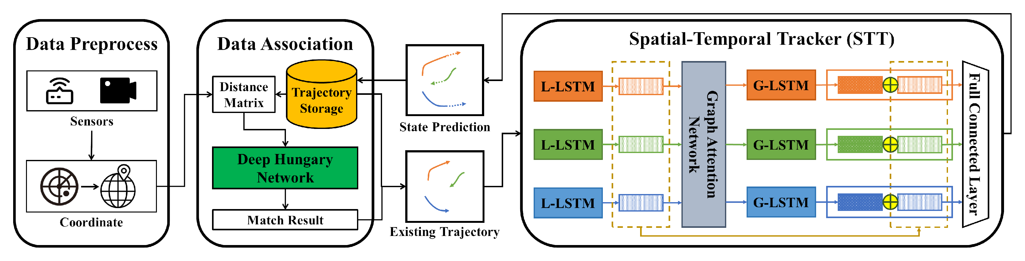
  • A multi-vehicle trajectory tracking framework for DT intersections (MVT2DTI) is proposed. It uses the proposed spatial–temporal tracker (STT) to model the interactions between the vehicles and their global motion patterns in IoV.
  • We utilize an improved tracking loss to back-propagate tracking errors. The tracking loss captures the impact of offset and loss in measurements to resolve the ID inconsistency of DT trajectories.
  • We generate four scene datasets on the trajectory data of Hangzhou city. Based on this, we validate the performance of the framework and further reveal the effectiveness of STT.
The rest of this article is organized as follows. Section 2 describes related work. Section 3 introduces some preliminary concepts. The proposed framework is described in detail in Section 4. Furthermore, Section 5 presents the experimental setup and verifies the proposed framework. Finally, Section 6 concludes this article.

2. Related Work

We surveyed existing tracking algorithms. Among them, the proposed framework focuses on two components, the data association algorithm, and the tracker. It should be noted that the scope of these works is broad and only those related to tracking will be reviewed.

2.1. Data Association

Since early detectors were noisy and unreliable, several approaches search for optimal data associations in offline or online computations and treat this as a network traffic optimization problem. Butt et al. [18] proposed a method for global multi-object tracking, where global matching is done with path estimation by preserving candidate pairs that match between consecutive frames. Schulter et al. [19] parametrize cost functions with neural networks with respect to the min-flow training objective. In addition, tracking can also find the optimal set of tracks through the conditional distribution of sequential track states, which is regarded as a maximum a posteriori (MAP) estimation problem. Choi et al. [20] propose to use long-term interest point trajectories to encode relative motion patterns between a pair of detections based on conditional random fields (CRFs). Ban et al. [21] propose an online variational Bayesian model for multi-person tracking, which yields a variational expectation-maximization (VEM) algorithm. Whether they are based on network traffic optimization or on the conditional distribution of sequential track states, the problem with these works is that the data association methods they propose are usually only partially trainable in terms of parameters. Moreover, these methods often are not generalizable and are bound to specific tracking algorithms.
Some recent works utilize neural networks to compute the affinity or association cost between extracted features, taking the output of the network as the input to the data association step. Milan et al. [22] construct a modified RNN for state prediction and a modified LSTM for data association, respectively, which completely rely on the ability of the neural network to complete the tracking step. Sun et al. [23] proposed Deep Affinity Network (DAN). The model detects multiple representations of objects by pre-learning so that the representations of the same object are as similar as possible in DAN, realizing deep learning-based affinity estimation across arbitrary frames. As the most traditional and general method, HA is difficult to integrate into deep networks due to its non-differentiability. Recently, Xu et al. [24] proposed the Deep Hungarian Network (DHN), which approximates the HA by pre-training the assignment results of the normalized matrix. Subsequently, other works expand and apply [25] based on DHN. These recent works show the great promise of neural networks in data association. Motivated by these works, this paper uses DHN to compute the distance matrix as an affinity matrix and propose an improved tracking loss applicable to the tracking of vehicle trajectories.

2.2. Tracker

The role of the tracker is to use the existing state of the tracked target for state estimation, which provides prior knowledge for subsequent steps.
The linear motion model is the first to appear. Breitenstein et al. [26] use the constant velocity assumption in their work. Based on this assumption, Milan et al. [27] model velocity smoothness in consecutive frames and force it to change smoothly. In addition, acceleration smoothness is also considered [28], which uses Gaussian distributions of displacement, velocity, and acceleration to calculate the next state estimation probability. Meanwhile, nonlinear motion models are proposed to describe more accurate motions. Yang et al. [29] applied a nonlinear motion model for tracking objects that move more freely. These methods are intuitive and simple, but their performance can be greatly compromised in complex scenarios.
With the increase of tracked targets, simple models cannot handle the interaction between multiple targets. To this end, an interaction model is applied to the tracking problem. Specifically, in the scene of pedestrians and vehicles, an object will be influenced by other objects, which is considered a social force [30]. Yuan et al. [12] manually modeled a group behavior model (GBM) as the inter-vehicle traffic force, and applied the GBM to Kalman filtering to predict the state of the vehicles. They argue that combining GBM with Kalman filtering can make predictions constrained by traffic rules, avoiding vehicle-to-vehicle collisions. Tian et al. [31] proposed a new Quasi-Bayesian adaptive method to update the transition probability matrix under the influence of multi-vehicle interactions. This is combined with prior information to compute longitudinal and lateral state estimates of the vehicle in a 2D coordinate system. All these methods are based on a priori knowledge for manual modeling of all parameters, which makes it difficult even for experts in the field to finalize the parameters for excellent performance.
With the development of deep neural networks, some works try to use them to learn the motion of objects, avoiding the limitations of manual modeling. Kim et al. [32] used a bilinear LSTM to learn long-term features for tracking objects. This tracking method can also be considered as a kind of MHT tracking framework [33]. Babaee et al. [34] used RNN to learn the motion of the target, thereby solving the occlusion problem. Chen et al. [11] implemented an attention network with LSTM units, making full use of historical and current information during tracking. To make full use of all the localization information, Wang et al. [13] proposed the LGM tracker, which completes the offline vehicle tracking task from a motion perspective without using appearance information. The neural network-based methods take little account of inter-vehicle interactions, which is complementary to the prior knowledge-based methods. Therefore, it brings us new ideas. Finally, Table 1 summarizes some of the most representative related works.

3. Preliminary

In this section, some symbols, definitions, and concepts will be introduced.
Definition 1 (Trajectory).
A vehicle trajectory is the driving route of a vehicle, represented as a sequence of GPS points with a time series. It should be noted that there are three types of vehicle trajectories described in this paper. The first type is the trajectory on the road, i.e., ground truth. The second type is the trajectory collected by the sensors, i.e, observations with errors. The third type is the tracked target trajectory connected by the data association algorithm, i.e., DT trajectories.
Definition 2 (Tracker).
It is a logical model for state prediction. Based on the state of the existing tracked target, the tracker needs to predict the future state to prepare for the matching at the next time step.
Definition 3 (Trajectory Storage).
It stores the trajectories of the tracked targets for the tracker’s state prediction and next matching. The extension of the stored trajectory indicates the movement trend of the DT trajectory.
Definition 4 (Tracking Errors).
The tracking errors represent the matching errors for DT trajectories, including false positive, false negative, and ID switch errors.
Problem Description: There are N vehicles in the scene during a time T and N t vehicles at time step t. Note that the number of vehicles may vary from time to time. For those vehicles, we employ o i t to denote the i-th collected observation at time step t, and O t = ( o 1 t , o 2 t , , o M t t ) to denote the observations collected for N t vehicles. Here, M t represents the number of observations with the time step t, which may not be equal to N t when some vehicles are missed. The goal is to match O t with O t 1 for the same vehicle. Finally, the DT trajectories mapped by the real trajectories are obtained.

4. Methodology

In this section, the tracker STT, the specific data association steps, and the DHN-based tracking loss are introduced sequentially. STT is introduced first because the computational flow is more intuitive this way. The proposed framework is shown in Figure 3.

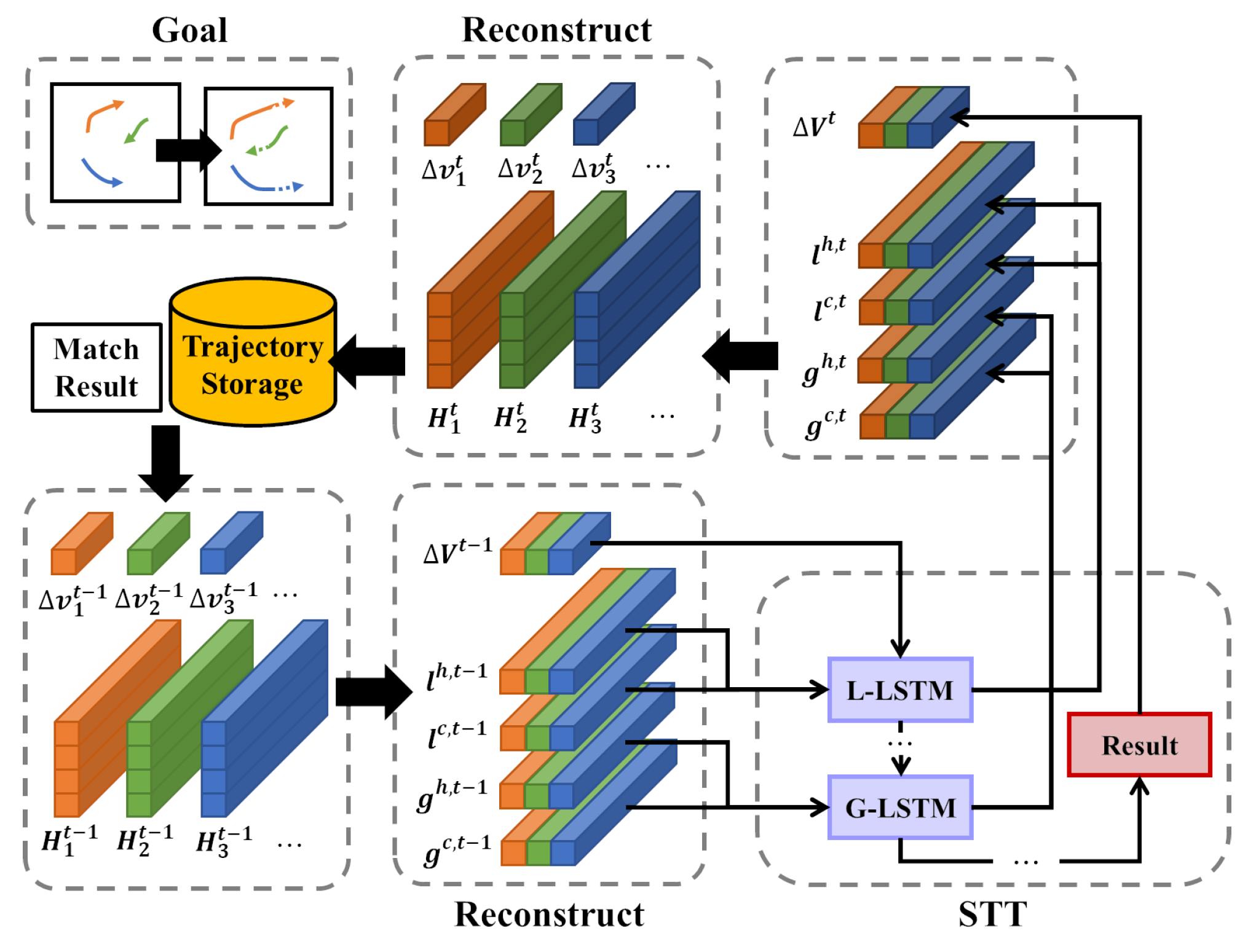
4.1. Spatial-Temporal Tracker (STT)

In the desired perfect case, the observations of the same vehicle in all time steps are correctly matched until the vehicle leaves the scene. However, the motion of a vehicle is complex and is usually affected by its own characteristics and other vehicles. Inspired by the work [35] and social properties, we implement a spatial–temporal feature fusion tracker STT.

4.1.1. Local Temporal Encoding

As we all know, drivers have their own driving habits, and vehicles also have their own hardware limitations, which can lead to different driving behaviors, including acceleration and speed. Considering that the state of the vehicle at the current time step will be affected by the previous, LSTM [36], a popular time series forecasting model, is used to model the temporal features of the vehicle, named L-LSTM (Local encoding LSTM).
In our implementation, before preparing to predict the next time step t, the relative displacement of the vehicle at time step t 1 is calculated first:
Δ l n g i t 1 = l n g i t 1 l n g i t 2
Δ l a t i t 1 = l a t i t 1 l a t i t 2
where l n g i t 1 and l a t i t 1 represent the longitude and latitude of the vehicle at time step t 1 , respectively. Δ l n g i t 1 and Δ l a t i t 1 represent the displacement. Then, the displacements are concatenated to the relative displacement vector Δ v i t 1 , which is input to the L-LSTM cell:
Δ v i t 1 = Δ l n g i t 1 Δ l a t i t 1
l i h , t , l i c , t = L - LSTM ( l i h , t 1 , l i c , t 1 , Δ v i t 1 ; W l , b l )
where ‖ represents the concatenation operation. l i h , t and l i c , t represent the L-LSTM hidden state and cell state of vehicle i at time step t, respectively. W l and b l are the weight and bias of the L-LSTM cell, and their values are adjusted during training and shared among all vehicles in the scene. At this point, l i h , t is local temporal embedding.

4.1.2. Spatial Encoding

The driving of the vehicle on the road is affected by other vehicles; for example, the vehicle may slow down due to the interference of other vehicles. Simply using an LSTM for each vehicle does not capture interactions between vehicles. The previous work [37] proposed the GAT model, which follows a self-attention strategy when computing graph-structured data, by assigning different attention coefficients to adjacent graph nodes to represent different importance. Meanwhile, another work [38] mentioned that the multi-head attention mechanism can stabilize the learning process of self-attention. It allows nodes to adopt different attention coefficients for neighbor nodes and uses a multi-head mechanism to set multiple assignment schemes. With these schemes, the features of neighbor nodes are aggregated and concatenated as the output. In this paper, with the help of sensors and IoV communication in the scene, connected vehicles are able to obtain the local temporal embedding of other vehicles in real-time and encode it with spatial information, as shown in Figure 4.
In our implementation, l i h , t is fed into the GAT, which outputs spatial embedding based on different attention coefficients. First, the attention coefficient of node j to i at time step t can be calculated by:
α i j t = exp LeakyReLU ( a T [ W l i h , t W l j h , t ] k N i exp LeakyReLU ( a T [ W l i h , t W l k h , t ] ,
where α i j t is the attention coefficient of node j to i at time step t. · T represents matrix transposition. N i represents the set of neighbor nodes of node i on the graph. W R F × F is a weight matrix shared by all nodes, which is used to linearly transform the features of each node, where F is the dimension of l i h , t , F is the dimension of output. a R 2 F is a shared attentional mechanism for computing attention coefficients. Then, the attention coefficients are normalized by the function LeackyReLU and softmax.
Then, the neighbor node features of each node need to be aggregated relying on the attention coefficient. To make the calculation step more stable, K independent attention mechanisms are used to transform the features of each node, which are then concatenated to obtain the output features, as follows:
s i t = k = 1 K σ j N i α i j t k W k l j h , t
where ‖ represents concatenation. σ is a nonlinear function. α i j t k is the normalized attention coefficient calculated by the k-th attention mechanism. The corresponding W k is the weight matrix of the linear transformation of the input.
Equations (5) and (6) form a single graph attention layer. In our practice, two graph attention layers are employed. The first layer uses a multi-head attention mechanism to explore the feasibility of various attention coefficients, while the second layer further aggregates the output of the first layer to obtain s i t , which we regard as spatial embedding. It represents the aggregate hidden state of vehicle i at time step t, including potential influences from other vehicles.

4.1.3. Global Temporal Encoding and Output

Assume that potential interactions between vehicles are successfully captured. However, for drivers in the real environment, there is a lag in their perception and response to the environment. Besides, GAT cannot memorize historical interaction information. Based on this fact, LSTM is used again, named G-LSTM (Global encoding LSTM), to perform temporal feature extraction on s i t :
g i h , t , g i c , t = G - LSTM ( g i h , t 1 , g i c , t 1 , s i t ; W g , b g )
where g i h , t and g i c , t are the G-LSTM hidden state and cell state of vehicle i at time step t, respectively. W g and b g are the weight and bias of the G-LSTM cell. At this point, g i h , t is global temporal embedding.
Through Equations (4) and (7), the features modeled with L-LSTM and the features modeled with GAT and G-LSTM are obtained. Then, the addition operation is used to achieve the combination of features and get the fusion feature e i t :
e i t = l i h , t + g i h , t
At this time, for the fusion result e i t , g i h , t can be regarded as the residual of l i h , t . Finally, a fully connected layer is used to decode e i t to obtain the prediction result:
Δ v i t = FC ( e i t ; W f , b f )
where Δ v i t represents the relative position of the vehicle at time step t. W f and b f are the FC weight and bias.
Using the position x i t 1 and the relative position Δ v i t of the vehicle i, the framework get its predicted position x ^ i t and the predicted positions of all vehicles X ^ t by analogy.

4.1.4. Overall Process

For the implementation of real-time DT trajectories, in addition to the above steps, some implementation ideas and details are explained. Suppose the current process is after getting the matching result. At this point, the matching result is a one-to-one match between X ^ t of all tracked targets and O t at the same time. For example, if x ^ i t and o j t are a pair match, it means that the o j t is the successor of the trajectory of the i-th tracked target. Thus, the observation is added to the trajectory, extending the DT trajectory segment. Furthermore, in the implementation, for each observation that fails to match, a new starting trajectory is created to record it. Besides, for each tracked target that fails to match, the target’s state prediction at the current time step is added to the trajectory as a substitute for the observation. Meanwhile, the target records the consecutive unmatched count, which indicates the upper limit of the target’s matching loss. When the count exceeds the threshold ε , it is considered that the vehicle to which the trajectory belongs has exceeded the detection range. Consequently, the target trajectory is moved out of the trajectory storage.
After that, each target has a series of vehicle observations. They can be connected into the DT trajectories to reflect how the vehicle travels on the road. To realize single-step prediction, each tracked target has a tracking state H , which contains the hidden state and cell state of L-LSTM and G-LSTM. All element values of H of the initial target are set to 0. In the prediction process, Δ v i t 1 and H i t 1 are taken out, and H i t 1 is reconstructed into l i h , t 1 , l i c , t 1 , g i h , t 1 and g i c , t 1 , which are input to two LSTMs, respectively. Finally, the output is reconstructed into H i t and updated to the corresponding target with Δ v i t . The process is shown in Figure 5.

4.2. Loss

When training a prediction model, the distance between the prediction and the ground truth is usually used as a loss to improve the accuracy of the prediction. However, the goal is to improve the tracking performance of STT. Tracking accuracy is not the same as prediction accuracy, which also considers information such as the consistency of the tracking ID. A recent work [24] proposes a model DHN. It takes as input the distance matrix between predictions and observations from the same time step and outputs an affinity matrix of the same size. Inspired by the work, this paper reuses it by improving its tracking loss, making it applicable to a wider range of task scenes, and for training STT.

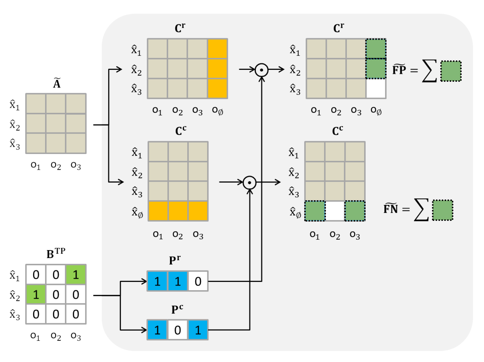
4.2.1. Distance Matrix

Since we only consider the location of vehicles, it is not possible to find an optimal ground truth bounding box for each predicted bounding box based on their feature affinity, i.e., IoU. The values in the distance matrix are defined as follows:
D r , c = ( x ^ r o c ) 2
D = β D
where D r , c represents the value in the r-th row and the c-th column in D . β is a scaling coefficient to normalize D . The result is scaled distance matrix D R L × M , where L represents the number of tracked targets while M represents the number of observations.
The Euclidean distance is calculated between state predictions and observations. Then, it is scaled so that the true positives of D are mainly distributed in the range of [ 0 , 0.1 ] , which is defined by the standard training set of DHN. The DHN takes D as input and output soft assignment matrix A ˜ [ 0 , 1 ] L × M .

4.2.2. Improved FP and FN

The definitions of FP ˜ and FN ˜ are further extended, considering the situation when the vehicle is missed or noise occurs. Figure 6 demonstrates the calculation process. Among them, C r [ 0 , 1 ] L × ( M + 1 ) is defined by the original work, which is obtained by filling a column of δ as a threshold after the last column of A ˜ and then applying softmax on the row dimension. The column x ^ where the threshold is located is filled with yellow. C c [ 0 , 1 ] ( L + 1 ) × M can be obtained by the same calculation in the column dimension. The row o where the threshold is located is filled with yellow. B TP is a binary matrix of the same size as A ˜ . The green-filled items indicate that the row and the column are a true positives match with a value of 1, while the white-filled items have a value of 0. P r is a one-dimensional matrix, whose non-zero entries signal rows in B TP with non-zero entry, represented by blue fill with a value of 1. Similarly, the non-zero entries of P c are the columns with non-zero entries in B TP .
Specifically, two mask matrices P r and P c are obtained through B TP . Then, mask it to C r and C c , respectively:
FP ˜ = n P 1 , n r × C n , o r
FN ˜ = m P 1 , m c × C x ^ , m c
Each n and m can get the matching error of a target and an observation, respectively. FP ˜ and FN ˜ indicates the sum of errors for targets and observations. The implication is that items whose tracker and observation are true positive matches should not be regard as false positives or false negatives.
Finally, the loss function is defined as:
d M O T A = 1 FP ˜ + FN ˜ + γ IDS ˜ M
d M O T P = D B TP 1 B TP 0
L t = λ 1 ( 1 d M O T A ) + λ 2 d M O T P
where IDS ˜ is the L1 norm of the Hadamard product of C 1 : L , 1 : M c and the binary complement of B TP . ⊙ denotes the Hadamard product. · 1 denotes the L1 norm of the matrix, while · 0 denotes the number of non-zero entries in the matrix. λ 1 and λ 2 is a loss balance factor. Minimizing this loss function is equivalent to penalizing the errors generated by false positives, false negatives, and ID switch errors.

4.3. Example

An example is used here to illustrate the capabilities of the proposed framework. Figure 7 shows the vehicle trajectories over a period of time, and other trajectories are not shown for clarity, where the numbers represent the IDs and the starting points of the trajectories. Vehicle No. 120 tries to overtake vehicle No. 119 from the right, vehicle No. 119 follows vehicle No. 114, and vehicle No. 122 tries to overtake vehicle No. 121 from the left. Similar to other neural networks, the proposed framework is mainly divided into two parts: model and loss. Specifically, the L-LSTM in the STT model captures the acceleration and deceleration information of the vehicle, and the GAT and G-LSTM capture the global feature information to achieve embedding spatiotemporal features. The proposed tracking loss strengthens the tracking ability on the basis of losing a certain prediction accuracy and allows STT to learn the ability through backpropagation. When only LSTM and prediction loss are used, higher prediction accuracy sometimes brings the paranoia of the model, that is, low error tolerance. Wrong predictions at this point will lead to mismatches and destruction. For example, the trajectory deflection of vehicles 120 and 122 when overtaking is difficult to predict accurately, but it can be matched and tracked.

5. Experiments

In this section, the dataset and experimental setup used in this paper is first introduced. Then, the extensive experiments are conducted to evaluate the proposed framework.

5.1. Hardware and Software Environments

The experiments are conducted on a computer with 256-GB memory, an Intel Xeon Gold 6130/2.1 GHz CPU, and a Quadro P6000/24 G GPU. Moreover, the proposed approach and all neural-network-based baseline models are implemented based on PyTorch 1.7.1 with the cuda101 using the Python language 3.6.13.

5.2. Dataset Description

Original Dataset.
The dataset used in the experiment is the vehicle trajectories provided by Zhejiang SUPCON Information Company, Ltd, which is China’s leading smart city solution and service provider. It includes a full day of trajectory data at the intersection of Binwen Road and Torch Avenue in Hangzhou on 10 May 2021. The data were sampled at a frequency of approximately 0.1 s, including sampled device information, vehicle appearance description, and positioning information. The decompressed file is about 7.9 GB in size and contains more than 80,000 trajectories, with an average of 600 records per trajectory. To obtain the ground truth as the original dataset, we remove the trajectories with missed intervals greater than five time steps and fill the missed records for the remaining trajectories using Lagrangian interpolation.
Extended Dataset.
In the real world, the signals captured by road sensors can generate errors in some cases, which are described in Section 1. To assess the effectiveness of the proposed framework more broadly, we intentionally manipulate the ground truth trajectories, making the data noisy to simulate sensor errors. Specifically, to construct a dataset that is similar to the real environment, this paper consider two crucial issues that arise with real-world sensors, namely offset and miss.
1.
Offset: So far in original datasets, vehicle trajectories are lowly biased. However, in the real world, the sensor may have coordinate offset due to its own hardware defects or the influence of external factors. We mimic this phenomenon by offsetting the original dataset with a Gaussian distribution with mean 0 and variance 10 5 under the world coordinates system.
2.
Miss: Sensor signal loss occurs when the vehicle is occluded or the signal is attenuated in a complex environment. We mimic this phenomenon by randomly dropping observations with a 10% probability in the original dataset and generating a missing dataset.
For brevity, we denote -O for offset datasets, -M for missing datasets, and -OM for datasets with both.

5.3. Experiment Settings

Metrics.
As the input to the proposed framework is multiple coordinates without IDs, while the output is the IDs assigned to observations by tracked targets whose state predictions are matched. Therefore, this paper use the following three metrics, i.e., MOTA, MOTP [39] and IDF1 [40], to evaluate the proposed method:
1.
Multiple Object Tracking Accuracy (MOTA): The measure combines three error sources: false positives, false negatives, and ID switch errors. The more the model is disturbed by errors, the worse the metric will be. It is one of the contributions that this paper needs to validate.
2.
Multiple Object Tracking Precision (MOTP): Due to the coordinate dataset, the experiments use the MOTP metric defined by [39], i.e., the average error in predicted positions for matched observation pairs over all frames. Through the metric, we will reveal that MOTP is not necessarily positively correlated with MOTA, thus validating the significance of the proposed tracking loss.
3.
ID F1 Score (IDF1): The ratio of correctly identified observations over the average number of ground truth and predicted positions. It is similar to MOTA as a combined metric, but differs in that it focuses on the continuous consistency of DT trajectory ID with the ground truth ID. It is also one of the contributions that need to be verified.
For the values of these metrics, higher is better on MOTA and IDF1, and lower is better on MOTP. In our practice, the units for MOTA and IDF1 are percentages, and for MOTP are 10 5 degrees of the coordinates system.
Parameters.
The key parameters of the proposed method are set as follows. All LSTMs are unidirectional and have one layer. Since their hidden state size requires a balance between performance and computation, as shown in Figure 8a, they are all set to 32. GAT is implemented as two layers, the first layer uses a four-head attention mechanism, and the second layer uses a single attention mechanism to aggregate the results of the first layer. In terms of additional parameters, ε is set to 0 without loss and set to 1 with loss, because the long-term loss involves the Reid field, which is beyond the research content of this work. The main purpose of β is to scale the distance matrix D to get the input of DHN, which needs to conform to the data distribution of the DHN standard training set. Considering the range of longitude and latitude displacements, as shown in Figure 8b, β is set to 10 4 . λ 1 and λ 2 used to balance the model loss function are set to 0.2 and 0.8, respectively. Finally, the model is optimized with the Adam optimizer, and learning rates are set to 1 × 10 2 , 3 × 10 2 , and 2 × 10 2 for the L-LSTM, GAT, and G-LSTM, respectively.
Baseline Model.
To verify the effectiveness of the proposed framework, we investigate several works that actively use motion models, comparing the proposed model with the motion models of the following methods:
1.
Linear Regression (LR): an LR with no other additional mechanisms, all trajectories are considered independent.
2.
Non-linear Motion (NLM) [29]: An extension to LR that considers motion patterns such as velocity, acceleration, etc.
3.
Group Behavior Model (GBM) [12]: It models the traffic force between vehicles and embeds the force in a Kalman filter to estimate the state of the target.
4.
RNN_LSTM [22]: It models an RNN-based architecture for state prediction, state update, and target existence probability estimation, and an LSTM-based model for data association.
5.
Multi Attention Module (MAM) [11]: It proposes a promoting tracking strategy that utilizes observations to generate a series of candidate targets to explore more possibilities.
The data association algorithm, except for the RNN_LSTM, uses the proposed LSTM, and all other methods use the most commonly used online data association algorithm HA.

5.4. Quantitative Evaluation

Table 2 shows the evaluation of MVT2DTI against all baseline models on four scene datasets. On the original dataset, it improves by 0.23% and 0.52% compared to the second place on MOTA and IDF1, respectively, and decreases by 20.0% on MOTP. Note that the improvement of MVT2DTI is significant on MOTP, but less on MOTA and IDF1.
On the original-O dataset, MVT2DTI is 2.12% lower than GBM on MOTA, but 39.6% lower on MOTP, and 1.39% higher on IDF1. A higher IDF1 indicates that it has better track ID consistency. A plausible explanation is that GBM captures the motion trend of the vehicle using the inter-vehicle force and Kalman filter, yet the trajectory ID that should have ended was wrongly assigned to another trajectory. MVT2DTI does this equally well and avoids vehicle ID switching. Compared with the original dataset, the advantage of MVT2DTI is reduced on MOTA, while it is improved on IDF1 and MOTP.
On the original-M dataset, compared to the second place, MVT2DTI improves by 3.11% and 1.79% on MOTA and IDF1 and reduces by 6.4% on MOTP. Compared with the original dataset, the advantage of it is slightly improved on MOTA and IDF1, while it is decreased on MOTP. Intuitively, since it has lower MOTP than other methods on the original dataset, it is better able to continue the motion trend of the vehicle when the signal loss occurs. However, it also relies on the ground truth to update the hidden state of the neural network, otherwise, its error will be amplified as the loss extends.
On the original-OM dataset, MVT2DTI improves by 0.38% and 7.04% on MOTA and IDF1, respectively, and reduces by 31.43% on MOTP. Compared to original-O and original-M datasets, it still maintains satisfactory performance.
Additionally, MVT2DTI is compared with an offline algorithm named LGM [13]. Since the offline algorithm needs to overlook all the frames or look ahead to a few frames to get future information, and the experiments take detection as an objective fact, the MOTP metric is meaningless here. The result is shown in Figure 9. In terms of MOTA, MVT2DTI is 3.25% and 5.31% lower than LGM on the two scenes, respectively. In terms of IDF1, it is 2.59% and 5.0% lower. The results on both datasets show the superior performance of the offline method, while MVT2DTI follows LGM. Even if MVT2DTI has no future information, it can learn the motion trend of the vehicle from the error data, which shows the stability.
Furthermore, considering that MVT2DTI is an online algorithm, we test the running time of each model under the same dataset containing 1131 trajectories, as shown in Table 3. The comprehensive results show that the computational efficiency of MVT2DTI is in the middle ranking, while the FPS still reaches a considerable level. It means that MVT2DTI can assign observations to the trajectories of tracked targets and complete a single-step prediction within the valid time frame, satisfying the real-time requirement of the DT system. This is due to the fact that MVT2DTI does not use a large-scale neural network, but a combination of several basic neural network components.

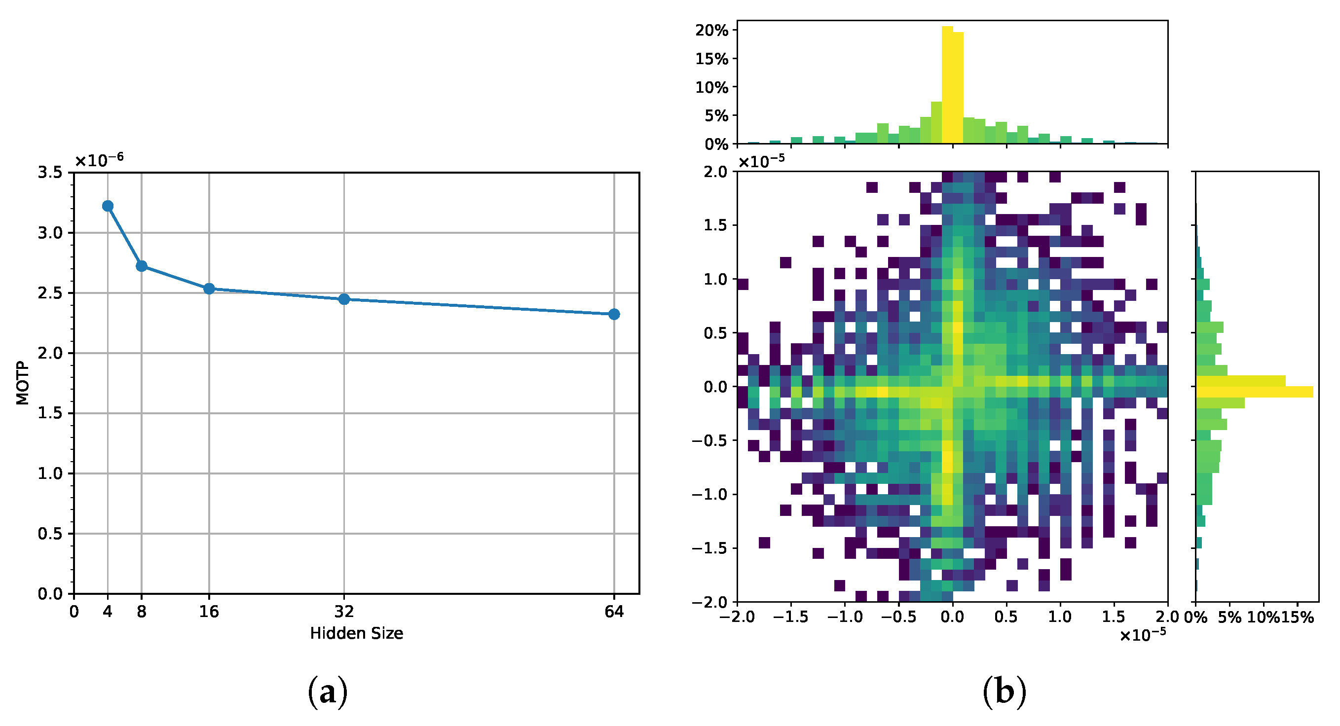
5.5. Component Analysis

To further understand the effect of each component of MVT2DTI, we conduct ablation experiments on it. MVT2DTI has two components, STT and the tracking loss L t . Hence, the ablation experiments are divided into the following groups. Firstly, a single LSTM is used to predict the target state, without GAT and the second LSTM, and is trained with L t (denoted as STT 1 + L t ). Secondly, a single LSTM and GAT are used to predict, without the second LSTM, and are trained with L t . The results of LSTM and GAT are added as Equation (8) (denoted as STT 12 + L t ). Thirdly, the assignment results are computed using HA and train STT using MOTP only (denoted as STT + L p ). The last one is MVT2DTI (denoted as STT + L t ). Therefore, experiments are conducted on four groups under two scene datasets to clarify the role of components in different scenes, as shown in Table 4.
For the performance comparison of STT 1 , STT 12 and STT under the two datasets. It can be noticed that under the original dataset, the GAT module optimizes the performance of a single LSTM, while STT outperforms the former two. Under the original-O dataset, the GAT module produces a serious error. At this time, a single LSTM module outperforms the GAT module, while STT still outperforms the other two. It shows that the GAT module can capture the interaction information between vehicles in normal scenarios, while inaccurate information in the scenario of offset data will lead to tracking errors. At this point, STT utilizes G-LSTM to share the GAT results at each moment to the global, thereby recovering its performance.
Comparing the performance of STT trained with L t and L p on the two datasets. It can be noticed that under the original dataset, the extra part in the tracking loss interferes with the training of the tracker because the wrong data is a small sample. Under the original-O dataset, IDF1 is improved because the tracking loss takes into account the impact of more misinformation on tracker training. Overall, STT outperforms individual components on both datasets, and the tracking loss strengthens the tracker in the presence of errors.

5.6. Discussion

To better understand the graph attention mechanism in STT, we select two sets of trajectories at different time periods and visualize their attention weight assignment scheme in Figure 10.
Figure 10a–d,f–i show the four attention weight assignment schemes obtained by the first layer multi-head attention mechanism of the two trajectories, respectively. Note that for the same trajectory, the four attention weight assignment schemes show drastically different results, indicating that the multi-head attention mechanism tries different assignment schemes for more possibilities. However, this also brings unstable attention weights. Figure 10a,f assigns more weights to nearby trajectories. Figure 10c,h tries to assign more weights to further but opposite trajectories, while Figure 10b,i assigns almost the same weights to all trajectories.
Therefore, the second layer uses a single attention mechanism to assign more reasonable attention weights to each trajectory. Figure 10j assigns higher weights to trajectories in the same direction, especially a trajectory in front of the target trajectory, and assigns relatively lower weights to trajectories in the opposite direction. Figure 10e assigns higher weights to trajectories in the same direction and assigns lower weights to the farthest trajectories in the opposite direction. Although the final attention weight assignments become more stable and reasonable, there are still problems that need to be pointed out. Figure 10e assigns a lower weight to adjacent trajectories than other trajectories at some time steps. Figure 10j assigns a lower weight to another trajectory ahead. Besides, the weights they assign on certain trajectories do not change smoothly at adjacent time steps. The first problem shows that although the second layer of the graph attention model can stabilize the attention weight assignment scheme, it cannot achieve perfect performance. The reason is MVT2DTI only takes the relative displacement as input, so the weights it learns are more about the motion trend of the vehicle. The second problem shows that GAT is not sensitive to time factors, which further shows the importance of using G-LSTM to encode GAT results so that the results can incorporate more time-step information.

6. Conclusions

In this work, we propose a framework for vehicle trajectory tracking at intersections with the help of IoV communication, paving the way for DT intersections. The framework’s STT embeds GAT using a multi-head attention mechanism on LSTM to improve the tracker’s ability to capture spatial–temporal features. Additionally, a new tracking loss is proposed and used to train the tracker. Finally, under the iteration of data input, data association, and state prediction, the unlabeled observations are connected as DT trajectories to reflect their real motion pattern. While the model focuses on the vehicle interactions and sampling errors that often occur at intersections, it can be applied to other road scenarios as well. In the future, for the framework that accepts relative displacement as input, we will consider some normalization methods and carefully try to introduce inter-vehicle distances. In addition, we will consider applying the framework to city-level road networks. At that time, the time complexity of calculation will strictly limit the number of vehicles. We will do more research to maintain the balance between efficiency and performance, and edge computing is considered promising.

Author Contributions

Conceptualization, Z.J., G.S. and J.W.; methodology, Z.J., M.C., Z.L. and X.K.; software, Z.J. and J.W.; validation, J.W.; formal analysis, Z.J. and J.W.; investigation, Z.J.; data curation, G.S.; writing—original draft preparation, Z.J. and J.W.; writing—review and editing, G.S., Z.L. and X.K.; funding acquisition, G.S., Z.L. and X.K. All authors have read and agreed to the published version of the manuscript.

Funding

This work was supported in part by the “Pioneer” and “Leading Goose” R&D Program of Zhejiang under Grant 2022C01050, in part by the Zhejiang Provincial Natural Science Foundation under Grant LR21F020003, and in part by the National Natural Science Foundation of China under Grant 62072409 and Grant 62073295.

Data Availability Statement

The data presented in this study are available on request from the corresponding author. The data are not publicly available due to privacy.

Conflicts of Interest

The authors declare no conflict of interest.

References

  1. Kong, X.; Zhu, B.; Shen, G.; Workneh, T.C.; Ji, Z.; Chen, Y.; Liu, Z. Spatial-Temporal-Cost Combination Based Taxi Driving Fraud Detection for Collaborative Internet of Vehicles. IEEE Trans. Ind. Inform. 2022, 18, 3426–3436. [Google Scholar] [CrossRef]
  2. Javed, A.R.; Faheem, R.; Asim, M.; Baker, T.; Beg, M.O. A smartphone sensors-based personalized human activity recognition system for sustainable smart cities. Sustain. Cities Soc. 2021, 71, 102970. [Google Scholar] [CrossRef]
  3. Javed, A.R.; Shahzad, F.; ur Rehman, S.; Zikria, Y.B.; Razzak, I.; Jalil, Z.; Xu, G. Future smart cities: Requirements, emerging technologies, applications, challenges, and future aspects. Cities 2022, 129, 103794. [Google Scholar] [CrossRef]
  4. Kong, X.; Duan, G.; Hou, M.; Shen, G.; Wang, H.; Yan, X.; Collotta, M. Deep Reinforcement Learning-Based Energy-Efficient Edge Computing for Internet of Vehicles. IEEE Trans. Ind. Inform. 2022, 18, 6308–6316. [Google Scholar] [CrossRef]
  5. Kong, X.; Wu, Y.; Wang, H.; Xia, F. Edge Computing for Internet of Everything: A Survey. IEEE Internet Things J. 2022, 9, 23472–23485. [Google Scholar] [CrossRef]
  6. Sun, W.; Lei, S.; Wang, L.; Liu, Z.; Zhang, Y. Adaptive Federated Learning and Digital Twin for Industrial Internet of Things. IEEE Trans. Ind. Inform. 2021, 17, 5605–5614. [Google Scholar] [CrossRef]
  7. Wu, Y.; Zhang, K.; Zhang, Y. Digital Twin Networks: A Survey. IEEE Internet Things J. 2021, 8, 13789–13804. [Google Scholar] [CrossRef]
  8. Kong, X.; Chen, Q.; Hou, M.; Rahim, A.; Ma, K.; Xia, F. RMGen: A Tri-Layer Vehicular Trajectory Data Generation Model Exploring Urban Region Division and Mobility Pattern. IEEE Trans. Veh. Technol. 2022, 71, 9225–9238. [Google Scholar] [CrossRef]
  9. Wang, J.; Fu, T.; Xue, J.; Li, C.; Song, H.; Xu, W.; Shangguan, Q. Realtime wide-area vehicle trajectory tracking using millimeter-wave radar sensors and the open TJRD TS dataset. Int. J. Transp. Sci. Technol. 2022. [Google Scholar] [CrossRef]
  10. Luo, W.; Xing, J.; Milan, A.; Zhang, X.; Liu, W.; Kim, T.K. Multiple object tracking: A literature review. Artif. Intell. 2021, 293, 103448. [Google Scholar] [CrossRef]
  11. Chen, B.; Li, P.; Sun, C.; Wang, D.; Yang, G.; Lu, H. Multi attention module for visual tracking. Pattern Recognit. 2019, 87, 80–93. [Google Scholar] [CrossRef]
  12. Yuan, Y.; Lu, Y.; Wang, Q. Tracking as a whole: Multi-target tracking by modeling group behavior with sequential detection. IEEE Trans. Intell. Transp. Syst. 2017, 18, 3339–3349. [Google Scholar] [CrossRef] [Green Version]
  13. Wang, G.; Gu, R.; Liu, Z.; Hu, W.; Song, M.; Hwang, J.N. Track without Appearance: Learn Box and Tracklet Embedding with Local and Global Motion Patterns for Vehicle Tracking. In Proceedings of the IEEE/CVF International Conference on Computer Vision, Montreal, QC, Canada, 11–17 October 2021; pp. 9876–9886. [Google Scholar]
  14. Kuhn, H.W. The Hungarian method for the assignment problem. Nav. Res. Logist. Q. 1955, 2, 83–97. [Google Scholar] [CrossRef] [Green Version]
  15. Lu, Z.; Rathod, V.; Votel, R.; Huang, J. Retinatrack: Online single stage joint detection and tracking. In Proceedings of the IEEE/CVF Conference on Computer Vision and Pattern Recognition, Seattle, WA, USA, 14–19 June 2020; pp. 14668–14678. [Google Scholar]
  16. Kong, X.; Wang, K.; Hou, M.; Hao, X.; Shen, G.; Chen, X.; Xia, F. A Federated Learning-Based License Plate Recognition Scheme for 5G-Enabled Internet of Vehicles. IEEE Trans. Ind. Inform. 2021, 17, 8523–8530. [Google Scholar] [CrossRef]
  17. Kong, X.; Wang, K.; Wang, S.; Wang, X.; Jiang, X.; Guo, Y.; Shen, G.; Chen, X.; Ni, Q. Real-time mask identification for COVID-19: An edge-computing-based deep learning framework. IEEE Internet Things J. 2021, 8, 15929–15938. [Google Scholar] [CrossRef] [PubMed]
  18. Butt, A.A.; Collins, R.T. Multi-target tracking by lagrangian relaxation to min-cost network flow. In Proceedings of the IEEE Conference on Computer Vision and Pattern Recognition, Portland, OR, USA, 23–28 June 2013; pp. 1846–1853. [Google Scholar]
  19. Schulter, S.; Vernaza, P.; Choi, W.; Chandraker, M. Deep network flow for multi-object tracking. In Proceedings of the IEEE Conference on Computer Vision and Pattern Recognition, Honolulu, HI, USA, 21–26 July 2017; pp. 6951–6960. [Google Scholar]
  20. Choi, W. Near-Online Multi-Target Tracking With Aggregated Local Flow Descriptor. In Proceedings of the IEEE International Conference on Computer Vision (ICCV), Santiago, Chile, 7–13 December 2015. [Google Scholar]
  21. Ban, Y.; Ba, S.; Alameda-Pineda, X.; Horaud, R. Tracking multiple persons based on a variational bayesian model. In Proceedings of the European Conference on Computer Vision, Amsterdam, The Netherlands, 8–16 October 2016; Springer: Cham, Switzerland, 2016; pp. 52–67. [Google Scholar]
  22. Milan, A.; Rezatofighi, S.H.; Dick, A.; Reid, I.; Schindler, K. Online multi-target tracking using recurrent neural networks. In Proceedings of the Thirty-First AAAI Conference on Artificial Intelligence, San Francisco, CA, USA, 4–9 February 2017. [Google Scholar]
  23. Sun, S.; Akhtar, N.; Song, H.; Mian, A.; Shah, M. Deep Affinity Network for Multiple Object Tracking. IEEE Trans. Pattern Anal. Mach. Intell. 2021, 43, 104–119. [Google Scholar] [CrossRef] [Green Version]
  24. Xu, Y.; Osep, A.; Ban, Y.; Horaud, R.; Leal-Taixé, L.; Alameda-Pineda, X. How to train your deep multi-object tracker. In Proceedings of the IEEE/CVF Conference on Computer Vision and Pattern Recognition, Seattle, WA, USA, 14–19 June 2020; pp. 6787–6796. [Google Scholar]
  25. Martija, M.A.M.; Naval, P.C. SynDHN: Multi-Object Fish Tracker Trained on Synthetic Underwater Videos. In Proceedings of the 2020 25th International Conference on Pattern Recognition (ICPR), Milan, Italy, 10–15 January 2021; IEEE: Piscataway, NJ, USA, 2021; pp. 8841–8848. [Google Scholar]
  26. Breitenstein, M.D.; Reichlin, F.; Leibe, B.; Koller-Meier, E.; Van Gool, L. Robust tracking-by-detection using a detector confidence particle filter. In Proceedings of the 2009 IEEE 12th International Conference on Computer Vision, Kyoto, Japan, 29 September–2 October 2009; pp. 1515–1522. [Google Scholar]
  27. Milan, A.; Roth, S.; Schindler, K. Continuous Energy Minimization for Multitarget Tracking. IEEE Trans. Pattern Anal. Mach. Intell. 2014, 36, 58–72. [Google Scholar] [CrossRef]
  28. Kuo, C.H.; Nevatia, R. How does person identity recognition help multi-person tracking? In Proceedings of the CVPR 2011, Colorado Springs, CO, USA, 20–25 June 2011; IEEE: Piscataway, NJ, USA, 2011; pp. 1217–1224. [Google Scholar]
  29. Yang, B.; Nevatia, R. Multi-target tracking by online learning of non-linear motion patterns and robust appearance models. In Proceedings of the 2012 IEEE Conference on Computer Vision and Pattern Recognition, Providence, RI, USA, 16–21 June 2012; IEEE: Piscataway, NJ, USA, 2012; pp. 1918–1925. [Google Scholar]
  30. Helbing, D.; Molnár, P. Social force model for pedestrian dynamics. Phys. Rev. E 1995, 51, 4282–4286. [Google Scholar] [CrossRef] [Green Version]
  31. Tian, Z.; Li, Y.; Cen, M.; Zhu, H. Multi-vehicle tracking using an environment interaction potential force model. IEEE Sens. J. 2020, 20, 12282–12294. [Google Scholar] [CrossRef]
  32. Kim, C.; Li, F.; Rehg, J.M. Multi-object tracking with neural gating using bilinear lstm. In Proceedings of the European Conference on Computer Vision (ECCV), Munich, Germany, 8–14 September 2018; pp. 200–215. [Google Scholar]
  33. Reid, D. An algorithm for tracking multiple targets. IEEE Trans. Autom. Control 1979, 24, 843–854. [Google Scholar] [CrossRef]
  34. Babaee, M.; Li, Z.; Rigoll, G. Occlusion handling in tracking multiple people using RNN. In Proceedings of the 2018 25th IEEE International Conference on Image Processing (ICIP), Athens, Greece, 7–10 October 2018; IEEE: Piscataway, NJ, USA, 2018; pp. 2715–2719. [Google Scholar]
  35. Huang, Y.; Bi, H.; Li, Z.; Mao, T.; Wang, Z. STGAT: Modeling Spatial-Temporal Interactions for Human Trajectory Prediction. In Proceedings of the IEEE/CVF International Conference on Computer Vision (ICCV), Seoul, Republic of Korea, 27 October–2 November 2019; pp. 6272–6281. [Google Scholar]
  36. Hochreiter, S.; Schmidhuber, J. Long Short-Term Memory. Neural Comput. 1997, 9, 1735–1780. [Google Scholar] [CrossRef] [PubMed]
  37. Veličković, P.; Cucurull, G.; Casanova, A.; Romero, A.; Liò, P.; Bengio, Y. Graph Attention Networks. In Proceedings of the International Conference on Learning Representations, Vancouver, BC, Canada, 30 April–3 May 2018. [Google Scholar]
  38. Vaswani, A.; Shazeer, N.; Parmar, N.; Uszkoreit, J.; Jones, L.; Gomez, A.N.; Kaiser, L.u.; Polosukhin, I. Attention is All you Need. In Proceedings of the Advances in Neural Information Processing Systems, Long Beach, CA, USA, 4–9 December 2017; Curran Associates, Inc.: Red Hook, NY, USA, 2017; Volume 30. [Google Scholar]
  39. Bernardin, K.; Stiefelhagen, R. Evaluating multiple object tracking performance: The clear mot metrics. EURASIP J. Image Video Process. 2008, 2008, 246309. [Google Scholar] [CrossRef]
  40. Ristani, E.; Solera, F.; Zou, R.; Cucchiara, R.; Tomasi, C. Performance measures and a data set for multi-target, multi-camera tracking. In Proceedings of the European Conference on Computer Vision, Amsterdam, The Netherlands, 8–16 October 2016; Springer: Cham, Switzerland, 2016; pp. 17–35. [Google Scholar]
Figure 1. Illustration of mapping the real-world intersection to the DT intersection via IoV communication.
Electronics 12 00275 g001
Figure 2. Four cases illustrating tracker-to-target assignments. (a) False positive and ID switch occur when vehicles change lanes. (b) False positive, false negative and ID switch occur when the vehicle turns. (c) Data loss occurs when the road sensor loses the vehicle signal. (d) Road sensors acquire vehicle signals with offset noise.
Electronics 12 00275 g002
Figure 3. Overview of the proposed framework.
Electronics 12 00275 g003
Figure 4. An illustration of multi-head attention with a single graph attention layer.
Electronics 12 00275 g004
Figure 5. Process of the single time step.
Electronics 12 00275 g005
Figure 6. Improved FP and FN.
Electronics 12 00275 g006
Figure 7. The vehicle trajectories at intersections over time.
Electronics 12 00275 g007
Figure 8. (a) The effect of hidden size on MOTP. (b) Distribution of longitude–latitude displacements.
Electronics 12 00275 g008
Figure 9. Performance comparison of LGM and MVT2DTI.
Electronics 12 00275 g009
Figure 10. Attention weights assigned by the graph attention mechanism. (aj) The five figures in each row show five attention weights assignment schemes for the same trajectory, i.e., four attention weights assignment schemes for the first layer and one for the second layer. The solid dots show the vehicle positions at different time steps, and the arrows show the direction. The color of the circle shows the time step, and its size shows the attention weight of the vehicle to a vehicle without circles on its trajectory.
Electronics 12 00275 g010
Table 1. Summary of selected related work.
ReferenceApproachLimitationsSimilarity/Dis-Similarity with Our Approach
[11]They implemented an attention network with LSTM units, making full use of historical and current information during tracking.It is unaware of the surrounding influences. The data association algorithm is independent of the tracker.Both use LSTM to capture temporal information.
[12]They manually modeled a group behavior model (GBM) as the inter-vehicle traffic force and applied the GBM to Kalman filtering to predict the state of the vehicles.It is difficult to finalize the parameters for excellent performance. The data association algorithm is independent of the tracker.Both consider inter-vehicle interactions.
[13]They proposed LGM, which gains more knowledge by looking ahead to future observations.Cannot be applied in the online stream. High computational consumption.Both combined the tracker and the data association algorithm, but in very different ways.
[21]They propose an online variational Bayesian model for multi-person tracking, which yields a variational expectation-maximization (VEM) algorithm.The data association algorithm is independent of the tracker. Deep learning methods were not used.Both are online algorithms.
[23]They proposed DAN, which detects multiple representations of objects by pre-learning so that the representations of the same object are as similar as possible, realizing deep learning-based affinity estimation across arbitrary frames.The representations of the tracked objects need to be prepared in advance for training data association components.Both combined the tracker and the data association algorithm, but the two components are trained in opposite directions.
Table 2. The performances of all the baseline models and MVT2DTI under the three metrics on four scene datasets.
ModelOriginalOriginal-OOriginal-MOriginal-OM
MOTAMOTPIDF1MOTAMOTPIDF1MOTAMOTPIDF1MOTAMOTPIDF1
LR92.400.57085.5185.381.80668.4571.580.57464.3958.321.86347.54
NLM95.040.29793.4959.482.13247.2176.100.32276.5716.342.25730.89
GBM95.010.35894.3892.241.33684.8275.270.40777.0972.981.38465.67
RNN_LSTM93.710.36294.1489.401.34870.3270.260.41271.6665.971.39557.11
MAM95.340.29493.9389.981.62575.5377.980.31678.4069.181.64458.10
MVT2DTI95.570.24594.9090.120.95786.2181.090.29780.1973.361.05372.71
Table 3. The comparison of model processing speed in seconds.
MetricsLRGBMRNN_LSTMMAMLGMMVT2DTI
Total28.4265.0531.41153.65351.2568.66
Time Usage2.29×1.11×5.41×12.36×2.42×
FPS175.976.9159.232.514.272.8
Table 4. Ablation experiments on individual components of MVT2DTI.
ModelOriginalOriginal-O
MOTAMOTPIDF1MOTAMOTPIDF1
STT 1 + L t 94.96%0.21293.14%89.82%0.89384.83%
STT 12 + L t 95.33%0.26394.25%87.81%1.36177.40%
STT + L p 95.81%0.23195.24%90.03%0.94985.59%
STT + L t 95.57%0.24594.90%90.12%0.95786.21%
Disclaimer/Publisher’s Note: The statements, opinions and data contained in all publications are solely those of the individual author(s) and contributor(s) and not of MDPI and/or the editor(s). MDPI and/or the editor(s) disclaim responsibility for any injury to people or property resulting from any ideas, methods, instructions or products referred to in the content.

