ROS Implementation of Planning and Robust Control Strategies for Autonomous Vehicles

Abstract

Autonomous vehicles are rapidly emerging as a crucial sector within the automotive industry. Several companies are investing in the development and enhancement of technologies, which presents challenging problems in the context of robotics and control. In particular, this work primarily focuses on the creation of an autonomous vehicle architecture utilizing the robotic operating system (ROS2) framework, accompanied by advanced control algorithms. In order to facilitate the development and implementation of lateral vehicle dynamics controllers, a reduced-size automated car available in GIPSA-Lab is used as an experimental platform. The objective is to design robust controllers capable of achieving optimal tracking and stability. Accordingly, this problem is tackled under different robust control syntheses, considering the $\mathcal{H}\infty$ approach: using linear time-invariant (LTI) and linear parameter-varying (LPV) model representations. Several simulation and experimental results are included to demonstrate the efficiency of the controllers.

1. Introduction

Autonomous systems, which are widely utilized in the current decade, have revolutionized the research and development sectors. Their applications span various fields, including industrial robotics, smart grids, drones, aerial vehicles, underwater vehicles, and self-driving cars. The fundamental principle behind these systems lies in their ability to react to the surrounding environment. Autonomous vehicles (AVs) have emerged as a pivotal domain within the automotive industry, prompting significant investments in their development. These vehicles offer a range of benefits, such as enhanced safety measures, reduced time and cost requirements, and alleviation of traffic congestion [1]. Undoubtedly, the technological advancements witnessed in the 21st century have played a major role in addressing the autonomous vehicle challenge.

Nowadays, it is feasible to implement real-time control closed-loop algorithms utilizing robust computing systems and reliable sensors. The International Society of Automotive Engineers (ISAE) classifies autonomy into five levels, each representing a step towards achieving a fully safe autonomous system [2]. Currently, companies are actively engaged in the pursuit of the third level, known as conditional automation. At this stage, the vehicle assumes control in all aspects; however, the driver must remain prepared to take over if necessary.

AVs possess the ability to interact with their environment and exhibit behavior akin to human actions. Consequently, it is imperative to develop various branches and sectors in a coherent manner to construct a safe and efficient AV system. Figure 1 illustrates the initial step involving sensing and perception, wherein the vehicle can discern different obstacles. Subsequently, it can make decisions and take actions to achieve its objectives through its own actuators and various transmission procedures [3]. Given the strong interconnection between scientific domains and industrial development sectors, extensive research communities are investigating all facets of autonomous vehicles. Advanced driver assistance systems (ADAS) represent a partial automation architecture designed to assist the driver [4], encompassing lane detection and tracking, lane departure warnings, blind-spot detection warnings, and collision-avoidance systems [5]. Moreover, the study of vehicle dynamics can be subdivided into two subdynamical systems capable of describing vehicle behavior as lateral and longitudinal dynamics. Considering the vehicle model and accounting for nonlinearities stemming from tire deformation or potential coupling between longitudinal dynamics, various controllers can be formulated to manage vehicle dynamics. In a comprehensive survey [6], a comparison of different control approaches was provided, highlighting the respective challenges and limitations inherent in each method. In the pursuit of managing nonlinearities that occur due to tire deformation and adapting to varying parameters in the vehicle’s dynamical model, an innovative data-driven control approach has emerged, as presented in [7]. This approach capitalizes on adaptive model-free control gain tuning by incorporating an extremum-seeking control (ESC) mechanism. The integration of an ESC enables real-time updates to the control gain of the controller, effectively adapting to dynamic changes in the system.

Adaptive cruise control (ACC) and cooperative adaptive cruise control (CACC) are employed to control the longitudinal dynamics of the vehicle while ensuring safety, comfort, and collision avoidance. Other control algorithms based on the robust ${\mathcal{H}}_{\infty }$ approach have been utilized [9,10,11]. Furthermore, model-based model predictive control (MPC) [12,13] has been experimentally verified as an efficient solution for managing longitudinal dynamics. On the other hand, the control of lateral dynamics is crucial for performing vehicle-tracking tasks, such as lane keeping and lane changes. Various techniques have been employed to manage these dynamics. The linear parameter-varying (LPV) framework, with its three different approaches—linear fractional transformation (LFT), polytope, and gridding methods—combined with the ${\mathcal{H}}_{\infty }$ approach, has been applied, with the results compared in [14]. In [15], the LPV polytope method was introduced, incorporating tracking errors with the look-ahead vision results [16]. A novel generalized plant with four states was obtained and controlled using the ${\mathcal{H}}_{\infty }$ approach. Moreover, a robust ${\mathcal{H}}_{\infty }$ controller with a polytopic gain approach was formulated in [17]. This controller was designed to achieve effective vehicle path tracking while addressing the nonlinearities present in the kinematic model. In a similar vein, ref. [18] tackles the issue of robust gain-scheduling control for path-following systems affected by network-induced delay. The authors employed linear fractional transformation to account for tire dynamics, proposed a generalized delay form, and presented a Markovian process. By utilizing a linear parameter-varying model, a robust gain-scheduling control method is introduced and subsequently validated through experimental trials involving autonomous vehicles.

The ${\mathcal{H}}_{\infty }$ approach was also proposed in [19,20] to control the vehicle’s steering angle. A comparison between LPV-MPC and nonlinear formulation approaches in controlling vehicle lateral dynamics is presented in [21,22]. Additionally, in [23], a new vehicle model that combines lateral and longitudinal dynamics is introduced, which is controlled using LPV-MPC approaches in a cascaded manner. Furthermore, in order to address path-following problems and enhance system robustness against uncertainties and varying parameters, a robust super-twisting sliding mode controller was employed in [24]. This controller leverages the Lyapunov function theory and has been experimentally validated to minimize lateral errors and improve the overall system robustness [25]. It is important to note that the implementation of these control algorithms in real-time applications presents an additional challenge in the development of autonomous vehicles. Organizing the work within a well-defined and well-treated architecture has been demonstrated to impact the execution of results [26,27].

In summary, the aforementioned control algorithms offer a range of potential solutions utilized in autonomous vehicles. However, selecting a robust controller that ensures stability of the vehicle’s yaw rate and effectively manages its dynamics remains a challenge within the automotive control community. This work encompasses both theoretical and practical aspects in the development of autonomous vehicles, as it involves various stages before designing a reliable control algorithm.

• Designing the ROS2 architecture: The initial focus is on developing the ROS2 architecture, taking into account technical implementation considerations. ROS2 serves as a crucial tool for testing of control algorithms. Although there has been some progress in implementing an autonomous vehicle architecture in ROS2, accomplishing this objective has proven challenging due to the variety of tasks involved. The framework will be utilized by colleagues to implement decision making and different vehicle lateral dynamic control algorithms.
• Estimating the lateral dynamics parameters of the new vehicle: With the introduction of a new vehicle, it is necessary to identify its model and estimate the lateral dynamics parameters. This step involves conducting multiple experiments, processing collected data, and addressing the mechanical aspects of the vehicle. Additionally, a realistic simulation is designed to test the controllers prior to implementation.
• Control of the lateral dynamics using a robust $\mathcal{H}\infty$ controller and planning algorithms: The final objective is to control the lateral dynamics of the vehicle utilizing a robust ${\mathcal{H}}_{\infty }$ controller and planning algorithms. This controller can be easily tuned and demonstrates good performance for linear systems. It also accounts for uncertainties and disturbances affecting the system. Furthermore, since the algorithm considers various system parameters, the LPV tool is tested to enhance vehicle tracking performance.

The implementation platform for testing the planned algorithms is an RC car available in the GIPSA-Lab. Different control strategies and robotic tools are employed to achieve closed-loop control of the system. However, prior to conducting experiments, the RC car requires initial modifications, including the addition of a differential system, measurement filtering, and generation the necessary reference signals for tracking.

The remainder of this article is structured as follows. The experimental platform is introduced in Section 2. The robust control methodology is detailed in Section 3. Section 4 provides an overview of the mathematical model and the system identification method employed to determine system parameters. The lateral control design is discussed in Section 5, which also includes the reference generation algorithm based on look-ahead vision. Ee present both experimental and simulation results in Section 6. Finally, the conclusion is provided in Section 7.

2. Experimental Setup

The GIPSA-Lab grounded vehicle platform offers researchers various tools to test their developed algorithms (

Table 1. RC car components.

	Type	Functionality
1	Swicth	Switching car power ON/OFF.
2	8 mm Qualisys super-spherical	Captured by Vicon tracker.
3	Arduino RP 2040	Microcontroller of the vehicle.
4	Spur gears	Increase torque provided by BLDC.
5	Elastic wheel	2 rear wheels of the vehicle.
6	ACCU NI-MH 3000	Supply battery power.
7	MG996R servo motor	Steering actuator.
8	Elastic wheel	2 Front wheels of the vehicle.
9	BLDC–A2212/13T	Throttle actuator.

). Figure 2 illustrates the components of the platform. It is equipped with a Vicon tracker comprising 12 cameras. This tracker enables the capture of precise position coordinates and the yaw angle of the vehicle, denoted as $(X_{\mathrm{global}},Y_{\mathrm{global}},\psi )$. A PC is utilized to run the control algorithms and associated codes within the framework of ROS2. It serves as the central processing unit for implementation and execution of the algorithms. The RC car used in the platform is equipped with an Arduino RP 2040 board. Communication between the Arduino RP 2040 board and ROS2 is established through a WiFi network. The RC car is equipped with two BLDC motors and one servo motor, enabling longitudinal and heading motions (see Figure 3 and Figure 4). The vehicle is also equipped with sensors for measuring battery voltage, current, and wheel encoders. The PC runs control algorithms at specified frequencies, sending PWM signals to the Arduino RP. The Arduino RP converts the signals into voltage inputs for the actuators. The resulting motion is captured by the Vicon tracker, which relays the information back to the PC.

Autonomous Vehicle ROS Implementation Framework

The overall system architecture comprises two main controllers: a high-level and low-level controller. The high-level controller generates actions and references for the vehicle’s actuators based on the sensed environment, objectives, and constraints. It is further divided into three primary blocks: detection, perception, and decision policy, as depicted in Figure 5. The sensing block collects and transmits necessary data to the perception node, which estimates the relevant states of the vehicle. The decision policy node functions as the vehicle’s brain, utilizing the obtained states and considering objectives to determine the optimal action to be conveyed to the lower controller. Within this architecture, the decision policy bears the responsibility of providing the reference longitudinal velocity ($v_x$) and the desired trajectory coordinates for the vehicle to follow. Path planning serves as a forward controller, translating the desired action into the heading rate reference (${\dot{\psi }}_{\mathrm{ref}}$) that the vehicle’s lateral dynamics track. Ultimately, the control algorithms are implemented in the control node, where commands for the lateral and longitudinal actuators are generated to guide the vehicle towards its objectives.

As previously mentioned, each component of this architecture operates on a specific node with a designated frequency. These nodes are interconnected through data exchange using defined topics through subscribing and publishing mechanisms. This framework facilitates the development of individual components by allowing modifications and updates to the running algorithms. As the paper’s direction suggests, the primary goal is to create a fundamental robust lateral controller that can be integrated into the mentioned architecture. In broad terms, the control gains are devised using MATLAB, while the implementation takes place using Python 3 within the ROS environment.

3. Control Theory

In the context of autonomous vehicles, it is crucial to employ a dynamic controller that offers robustness, stability, and accurate tracking in the presence of uncertainties and noise. Therefore, it is logical to choose an approach that can fulfill these requirements and fine tune it based on the specific application. This work emphasizes the utilization of $\mathcal{H}\infty$ control, which embodies principles that align with the aforementioned objectives. The aim is to explore the principles of ${\mathcal{H}}_{\infty }$ control and implement it in a real-time dynamic system. By doing so, the controller can effectively handle various challenges and disturbances encountered in autonomous vehicle applications.

3.1. Definition of ${\mathcal{H}}_{\infty }$ Norm

The ${\mathcal{H}}_{\infty }$ norm of a proper LTI system is defined by the state space representation $(A,B,C,D)$ from an input ($w\left(t\right)$) to an output ($z\left(t\right)$) that belongs to ${\mathcal{RH}}_{\infty }$, which is the induced energy to the energy gain, defined as:

$${\parallel G\left(j\omega \right)\parallel }_{\infty }=\underset{\omega \in \mathbb{R}}{sup}\overline{\sigma }\left[G\left(j\omega \right)\right]<\infty$$

(1)

${\mathcal{H}}_{\infty }$ is considered equivalent to the ${\mathcal{L}}_2$-induced norm.

3.2. ${\mathcal{H}}_{\infty }$ Control Problem Formulation

Here, we present the simple ${\mathcal{H}}_{\infty }$ control problem formulation that was used in this study. The target system to be controlled is represented in Figure 6 by $G\left(s\right)$. Two weighting functions ($W_e$ and $W_u$) act as tuning constraints for the built controller ($K\left(s\right)$). The scheme in Figure 6 is converted to the $LFT$ scheme shown in Figure 7.

The generalized plant (P) aims to characterize the controlled output with the external input and build a controller that minimizes the ${\mathcal{L}}_2$-induced gain from the external input ($\omega$) to the controlled output (e). In other words, the controller must minimize the impact of the reference and the assumed disturbances and noises with respect to the output of the defined weighting functions. The suboptimal ${\mathcal{H}}_{\infty }$ problem is formulated as shown in Equation (2). Given a positive value of $\gamma >0$, the objective is to compute a stabilizing controller ($K\left(s\right)$).

$${\parallel e\parallel }_2\le \gamma {\parallel \omega \parallel }_2,{\parallel T_{ew}\parallel }_{\infty }=∥\begin{array}{c}{W}_{e}S\\ W_{u}KS\end{array}∥\le \gamma$$

(2)

$$T=\frac{GK}{1-GK},S=1-\frac{GK}{1-GK},SG=S\times G,KS=K\times S$$

(3)

where S represents the sensitivity function that quantifies the impact of noise on the closed-loop($T_{yr}$), while $KS$ signifies the controlled sensitivity function that illustrates the influence of external input on the controlled input (u). A controller can be formulated to achieve a minimum ${\gamma }_{min}$ concerning the sensitivity functions, while adhering to defined templates. This task is addressed by either employing the algebraic Riccati approach or utilizing the linear matrix inequality (LMI) method, as outlined by Zhou, Skogestad, and Postlewaite). Weighting functions $W_e$ and $W_u$ defined as in Equation (4) are utilized to design templates for S and $KS$, respectively.

$$\frac{1}{W_e}=\frac{s+{\omega }_b{ϵ}_e}{\frac{s}{M_s}+{\omega }_b}\mathrm{and}\frac{1}{W_u}=\frac{{ϵ}_{u}s+{\omega }_{b}c}{s+\frac{{\omega }_{b}c}{M_u}}$$

(4)

The weighting function is tuned according to the required performance, where:

• $M_s$: Robustness required with max module margin;
• ${\omega }_b$: Tracking speed and rejecting disturbances;
• ${ϵ}_e$: Steady-state tracking error;
• $M_u$: Actuator constraints based on $\frac{\Delta u}{\Delta r}$;
• ${\omega }_{bc}$: Actuator bandwidth;
• ${ϵ}_u$: Attenuated noises on controlled input.

The plant (P) can be expressed in another form as shown in (5).

$$\begin{array}{cc}\hfill & \dot{x}=Ax+B_1\omega +B_{2}u\hfill \\ \hfill & e=C_{1}x+D_{11}\omega +D_{12}u\hfill \\ \hfill & y=C_{2}x+D_{21}\omega +D_{22}u\hfill \end{array}$$

(5)

where $x\in {\mathbb{R}}^n$ is the union of the plant states and the weighing function states, $\omega \in {\mathbb{R}}^{n_{\omega }}$ represents the defined external inputs to P, $u\in {\mathbb{R}}^{n_u}$ is the controlled input, $e\in {\mathbb{R}}^{n_e}$ represents the the controlled outputs, and $y\in {\mathbb{R}}^{n_y}$ represents the measured outputs of the system. In the context of the employed mixed-sensitivity problem, a stabilizing controller (K(s)) is computed to satisfy the following condition:

$${∥\begin{array}{c}{W}_{e}S\\ W_{u}KS\end{array}∥}_{\infty }\le 1$$

(6)

This implies a sufficient but not necessary condition, as shown in Equation (7).

$${∥\begin{array}{c}{W}_{e}S\end{array}∥}_{\infty }\le 1,{∥\begin{array}{c}{W}_{u}KS\end{array}∥}_{\infty }\le 1$$

(7)

3.3. LPV System Modeling Formulation

A dynamical system that includes varying parameters in its state-space model can be reformulated to be modeled as an LPV system. Different approaches deal with modeling formulation problems, such as gridding, LFT, and polytope approaches. The state space of the generalized LPV plant (P) is represented by (8).

$$\left[\begin{array}{c}\dot{x}\\ e\\ y\end{array}\right]=\left[\begin{array}{ccc}A\left(\rho \right)& B_1\left(\rho \right)& B_2\left(\rho \right)\\ C_1\left(\rho \right)& D_{11}\left(\rho \right)& D_{12}\left(\rho \right)\\ C_2\rho & D_{21}\left(\rho \right)& D_{22}\left(\rho \right)\end{array}\right]\left[\begin{array}{c}x\\ w\\ u\end{array}\right]$$

(8)

where $x\left(t\right)\in {\mathbb{R}}^n\cdots \rho =({\rho }_1\left(t\right),{\rho }_2\left(t\right),\cdots ..,{\rho }_N\left(t\right))\in \Omega$ is a vector of time-varying parameters, where $\Omega$ is a defined convex set, and $\rho (.)$ is assumed to be bounded and is known as $\rho \in \Omega \subset {\mathbb{R}}^N$.

3.3.1. Affine Parameter Dependence

The LPV system matrices can be written in the form of affine parameters (9).

$$A\left(\rho \right)=A_0+A_1{\rho }_1+\cdots +A_N{\rho }_N$$

(9)

3.3.2. Polytopic Modeling Approach

The polytopic modeling approach is another representation of an affine LPV system. Assuming that ${\rho }_i\in [\underline{{\rho }_i},\overline{{\rho }_i}]$, it is possible to build a polytope containing all possible ${\rho }_i$. Two main conditions must be satisfied [14]: the input and output matrices should be independent of the variable parameter, and the model must be affine with respect to the parameters. The variation of $\rho$ within the corners of the convex polytope problem is defined as $\rho ={\sum }_{i=1}^{2^{n_p}}{\mu }_i{\omega }_i$ and ${\sum }_{i=1}^{2^{n_p}}{\mu }_i=1$, where $n_p$ represents the number of varying parameters, and ${\mu }_i\ge 0$. Assuming that the targeted system contains two varying parameters (${\rho }_1$ and ${\rho }_2$), the convex optimization problem is formulated as a polytope with four corners, as shown in Figure 8 and defined by Equation (10).

$$\begin{array}{cc}\hfill & {\mu }_k=\frac{{\prod }_{j=1}^{n_p}|{\rho }_j-\mathcal{C}{\left({\omega }_k\right)}_j|}{{\prod }_{j=1}^{n_p}(\overline{{\rho }_j}-\underline{{\rho }_j})}\hfill \\ \hfill & \mathcal{C}{\left({\omega }_k\right)}_j=\left\{{\rho }_j\right|{\rho }_j=\overline{{\rho }_j}\mathrm{if}\left({\omega }_k\right)j=\underline{{\rho }_j}\&{\rho }_j=\underline{{\rho }_j}\mathrm{if}{\left({\omega }_k\right)}_j=\overline{{\rho }_j}\}\hfill \\ \hfill & {\omega }_1=(\underline{{\rho }_1},\underline{{\rho }_2}){\mu }_1=\frac{|\overline{{\rho }_1}-{\rho }_1|}{|\overline{{\rho }_1}-\underline{{\rho }_1}|}\times \frac{|\overline{{\rho }_2}-{\rho }_2|}{|\overline{{\rho }_2}-\underline{{\rho }_2}|}\hfill \\ \hfill & {\omega }_2=(\underline{{\rho }_1},\overline{{\rho }_2}){\mu }_2=\frac{|\overline{{\rho }_1}-{\rho }_1|}{|\overline{{\rho }_1}-\underline{{\rho }_1}|}\times \frac{|\underline{{\rho }_2}-{\rho }_2|}{|\overline{{\rho }_2}-\underline{{\rho }_2}|}\hfill \\ \hfill & {\omega }_3=(\overline{{\rho }_1},\underline{{\rho }_2}){\mu }_3=\frac{|\underline{{\rho }_1}-{\rho }_1|}{|\overline{{\rho }_1}-\underline{{\rho }_1}|}\times \frac{|\overline{{\rho }_2}-{\rho }_2|}{|\overline{{\rho }_2}-\underline{{\rho }_2}|}\hfill \\ \hfill & {\omega }_4=(\overline{{\rho }_1},\overline{{\rho }_2}){\mu }_4=\frac{|\underline{{\rho }_1}-{\rho }_1|}{|\overline{{\rho }_1}-\underline{{\rho }_1}|}\times \frac{|\underline{{\rho }_2}-{\rho }_2|}{|\overline{{\rho }_2}-\underline{{\rho }_2}|}\hfill \end{array}$$

(10)

The LPV model is created by solving the controller LTI problem at each vertex of the convex set, and by knowing the actually desired varying parameter ($\rho$), it is possible to schedule the needed controller. The interpolation between the four vertices is performed according to (11).

$$\left[\begin{array}{cc}{A}_{pol}\left(\rho \right)& B_{pol}\left(\rho \right)\\ C_{pol}\left(\rho \right)& D_{pol}\left(\rho \right)\end{array}\right]=\sum _{i=1}^{2^{n_p}}{\mu }_i\left(\rho \right)\left[\begin{array}{cc}A\left({\omega }_i\right)& B\left({\omega }_i\right)\\ C\left({\omega }_i\right)& D\left({\omega }_i\right)\end{array}\right]$$

(11)

4. Estimation of the Bicycle Lateral Model Parameters

4.1. Mathematical Modeling

Studying the behavior of a system while considering all the forces that influence it falls under the domain of system dynamics. In the case of autonomous vehicles, the dynamics of the system are significantly influenced by the forces exerted by the wheels. The motion of the vehicle can be effectively described by analyzing the behavior of the wheels from various perspectives. To simplify the modeling process, an assumption is made that the four wheels of the vehicle can be represented by two wheels. The individual front and rear wheels of the vehicle are then modeled accordingly, as depicted in Figure 9. This modeling approach is commonly referred to as the bicycle model. The model operates under the assumption that both the front and rear wheels move at the same angular speed. However, to account for the consequences of this assumption, a differential system is introduced. This system incorporates the steering angle ($\delta$) and calculates the velocity difference between the wheels. It is important to note that the bicycle model simplifies the system and subsequently streamlines the control design process. Moreover, it effectively captures the vehicle’s lateral dynamics. It is worth mentioning that these assumptions might impact the model’s performance when dealing with high velocities and drifting maneuvers, scenarios that are not relevant to the context of our controller design work. Nevertheless, the challenge of vehicle control involving drifting maneuvers and high slip angles was explored and applied in [30]. In their study, the authors devised a hierarchical dynamic drifting controller (HDDC) that comprises a path-tracking layer, a vehicle motion control layer, and an actuator regulation layer.

By applying Newton’s second law and summation of the moment around the axis of rotation of the vehicle, the mathematical model can be represented as shown in Equation (12).

$$\begin{array}{cc}\hfill & {\dot{v}}_y=-\frac{2C_f+2C_r}{m{v}_x}{v}_y-v_x\dot{\psi }-\frac{2C_f{l}_f-2C_r{l}_r}{m{v}_x}\dot{\psi }+\frac{2C_f}{m}\delta \hfill \\ \hfill & \ddot{\psi }=-\frac{l_{f}2C_f-l_{r}2C_r}{I_z{v}_x}{v}_y-\frac{l_{f}2C_f+l_{r}2C_r}{I_z{v}_x}\dot{\psi }+\frac{l_{f}2C_f}{I_z}\delta \hfill \end{array}$$

(12)

$$A=\left[\begin{array}{cc}-\frac{2C_f+2C_r}{m{v}_x}& v_x-\frac{2C_f{l}_f-2C_r{l}_r}{m{v}_x}\\ -\frac{l_{f}2C_f-l_{r}2C_r}{I_z{v}_x}& -\frac{l_{f}2C_f+l_{r}2C_r}{I_z{v}_x}\end{array}\right]B=\left[\begin{array}{c}\frac{2C_f}{m}\\ \frac{l_{f}2C_f}{I_z}\end{array}\right]$$

(13)

The system can be described by the state-space representation shown in Equation (13). The input to the system is the steering angle in radians, while the states are the lateral velocity ($v_y$) and the vehicle’s yaw rate ($\dot{\psi }$). The parameters that need to be identified include the front and rear wheel stiffness ($C_f$ and $C_r$, respectively), the position of the center of gravity (represented by the distances to the front wheels ($l_f$) and the rear wheels ($l_r$)), and the inertia around the axis of rotation ($I_z$).

4.2. System Identification

The chosen bicycle model is a linear model that incorporates a varying parameter ($v_x$). However, it is important to acknowledge that this model has certain limitations when it comes to describing the vehicle’s motion at low velocities and capturing the nonlinearities that may arise in the system. To address these limitations, LPV identification techniques can be employed. These techniques allow for the identification of both the state space and transfer functions of the system, as demonstrated in [32]. By utilizing LPV identification, a more accurate representation of the vehicle’s dynamics can be obtained, considering the varying parameters and nonlinear behaviors that may influence the system.

Within the field of system identification, diverse strategies can be employed to achieve favorable outcomes, contingent on the pre-existing understanding of the system. These strategies fall under categories such as black-box, gray-box, and white-box techniques [33]. Leveraging knowledge of the mathematical model governing the lateral dynamics of vehicles, gray-box identification techniques prove suitable for estimating unknown parameters of the model. Specifically, the prediction error method (PEM) is employed to minimize the disparity between measured and simulated outputs by adjusting these unknown parameters. However, it is acknowledged that this method is sensitive to initial conditions; the solver can become trapped in local optima associated with incorrect parameter estimates. To counter this, initial conditions are selected based on fundamental physical insights into the system. Data are collected through open-loop identification, involving step inputs consistently applied to stimulate the system, thereby activating all vehicle frequencies and dynamics.

In an experimental setup, a fixed PWM signal was applied to achieve a target angular speed of the wheel of $\dot{\theta }=25$ rad/s. Meanwhile, the longitudinal velocity of the vehicle varied between $v_x=1.1$ m/s and $v_x=1.3$ m/s. To control the steering angle ($\delta$) a joy-stick was utilized to provide different PWM signals. These PWM signals were converted into an input voltage that directly controlled the servo motor, allowing for precise manipulation of the steering angle.

After processing and filtering the collected data, an optimization problem is solved to address Equation (14), where y represents the actual measured data indicating the states of the bicycle model, and $\widehat{y}\left(\widehat{\varphi }\right)$ represents the simulated model states. The identification results are presented in Figure 10 and

Table 2. Vehicle parameter estimation.

Parameter	Value	S.I Units
m	$1.1937$	Kg
$I_z$	$0.005$	Kg·m${}^2$
$C_f$	$4.8438$	$\frac{N}{rad}$
$C_r$	$11.2441$	$\frac{N}{rad}$
$l_r$	$0.1049$	m
$l_f$	$0.0691$	m

. The analysis reveals that the input delay occurs between 9 and 13 sampling times in the system. The root mean square error (RMSE) is calculated to be $0.268$.

$$\underset{\widehat{\Phi }}{min}{\parallel y-\widehat{y}\left(\widehat{\varphi }\right)\parallel }_2\mathrm{Where}\widehat{\Phi }=[C_f,C_r,l_r,l_f,I_z]$$

(14)

To ensure that the estimated model closely approximates the actual system, it is crucial to validate the obtained outcomes. New data were gathered, and the estimated results were employed to simulate the system using real inputs. As depicted in Figure 11, the simulated outcomes align well with the measured outcomes, affirming that the identified system can effectively model the system’s dynamic behavior. Importantly, the main constraint of this identification technique lies in its inability to accurately model lateral dynamics across all variable $v_x$ values, as previously mentioned. This limitation arises from nonlinearities stemming from tire deformation. Nonetheless, the system is identified within the desired operational range of $v_x$.

5. Lateral Control Design

The lateral control architecture comprises two primary controllers: the reference generator and the feedback controller. The reference generator is responsible for generating a reference value (${\dot{\psi }}_{ref}$), which the vehicle must track. On the other hand, the feedback controller is responsible for regulating the vehicle’s dynamics to enable it to follow the desired trajectory.

5.1. Look-Ahead Reference Generator

Tracking $\dot{\psi }ref$ is the chosen method to track a defined path. Different methods can generate this reference based on human interaction while driving. Pure pursuit, Stanley, lateral error, and look-ahead vision are the most popular strategies that achieve satisfactory results in real implementation [15,34]. The philosophy of generating $\dot{\psi }ref$ is shown in Figure 12. The forward distance (L) from point A is tuned using (15); then, the nearest point on track B to C is found. With the coordinates of $(A,B,C)$ and knowing the $\psi$ of the vehicle, it is possible to generate ${\dot{\psi }}_{ref}$ using (16).

$$L=t_{p}V,t_p\mathrm{look}-\mathrm{ahead}\mathrm{time}\mathrm{to}\mathrm{be}\mathrm{tuned}.$$

(15)

$${\dot{\psi }}_{ref}=\frac{2Vsin\left(\alpha \right)}{L}\mathrm{where}\alpha =arctan\left(\frac{y_B-y_A}{x_B-x_A}\right)-\psi$$

(16)

5.2. $LTI/{\mathcal{H}}_{\infty }$ Controller

A robust ${\mathcal{H}}_{\infty }$ controller was chosen to regulate the lateral dynamics of the vehicle. In the initial step, the system is treated as an LTI system, neglecting variations in $v_x$. The controller is designed using the architecture depicted in Figure 6. Weighting functions $W_e$ and $W_u$ are designed as first-order transfer functions, as shown in Equation (4). Offline tuning of the parameters is performed, with specific values provided in

Table 3. Vehicle lateral dynamic ${\mathcal{H}}_{\infty }$ weighting parameters.

Parameter	Value
$M_s$	2
${\omega }_b$ (rad/s)	3.14
${ϵ}_e$	${10}^{-2}$
$M_u$	1
${\omega }_{bc}$ (rad/s)	31.4
${ϵ}_u$	${10}^{-3}$

. It is important to note that the controller is designed in discrete time. Both the weighting functions and the system are discretized using the Tustin method, with a sampling time of $T_s=0.02$.

To design the controller, the LMI approach is utilized, and the MATLAB Robust toolbox is employed to determine the optimal value of $\gamma$ (${\gamma }_{optimal}$). The response of the closed-loop system to frequency analysis is aligned with the predefined templates, exhibiting noise rejection capabilities and tracking the desired references, as shown in Figure 13.

5.3. $LPV/{\mathcal{H}}_{\infty }$ Controller

The longitudinal speed, denoted as $v_x$, is assumed to be bounded within the range of $0.4$ to $1.6$ m/s. A polytopic modeling approach is adopted, considering two independent parameters: ${\rho }_1=v_x$ and ${\rho }_2=\frac{1}{v_x}$. Figure 8 illustrates the four vertices that describe the convex formulation of the set. The $LPV/{\mathcal{H}}_{\infty }$ solution involves solving an LMI-based optimization method to find the controller ($K_i$) at each vertex of the polytope. Utilizing the tuned weighting functions provided in Table 3, four generalized plants are constructed at each corner of the polytope, denoted by ${\omega }_i$.

It is worth noting that the considered approach is deemed conservative, as it describes an excessively large set compared to the actual parameter variations [14]. To address this issue, the fourth vertex is eliminated, resulting in a total of $np+1$ vertices when determining the controller at specified $({\rho }_1,{\rho }_2)$. The new interpolation coefficients are represented in Equation (17).

$${\mu }_1=1-({\mu }_2+{\mu }_3),{\mu }_2=\frac{|\underline{{\rho }_2}-{\rho }_2|}{|\overline{{\rho }_2}-\underline{{\rho }_2}|},{\mu }_3=\frac{|\underline{{\rho }_1}-{\rho }_1|}{|\overline{{\rho }_1}-\underline{{\rho }_1}|}$$

(17)

The controller ($K\left(\rho \right)$) at the target point (${\rho }_1,{\rho }_2$) is then calculated using (18).

$$\left[\begin{array}{cc}{A}_K\left(\rho \right)& B_K\left(\rho \right)\\ C_K\left(\rho \right)& D_K\left(\rho \right)\end{array}\right]=\sum _{i=1}^{n_p+1}{\mu }_i\left(\rho \right)\left[\begin{array}{cc}{A}_{K_i}& B_{K_i}\\ C_{K_i}& D_{K_i}\end{array}\right]$$

(18)

6. Simulation and Experimental Results

The designed controller is implemented and simulated using the MATLAB Simulink simulator. The simulation architecture is depicted in Figure 14. The kinematic model is employed to determine the vehicle’s position during simulation time. The outputs ($\dot{X}$ and $\dot{Y}$) are integrated to obtain the global position of the vehicle $(X,Y)$ on the track. This model is typically utilized to describe the motion of a vehicle at low velocities. The servomotor actuator is modeled as a first-order transfer function, denoted as $G_{act}$, with an input delay. In the lateral model of the bicycle, ${\gamma }_c$ represents the controlled input, while $\delta$ represents the input for the steering angle. In this section, both simulation and experimental results are presented for analysis and comparison.

6.1. Simulation of LTI/${\mathcal{H}}_{\infty }$ Controller

The controller is designed assuming a constant velocity of $v_x=1$ m/s. The tracking results are presented in Figure 15. The simulated system demonstrates accurate path following. The observed oscillation at the end of the first lap is attributed to the vehicle’s speed transitioning from curvature following to straight-line following. In the simulation, $v_x$ is varied between 0.8 and 1 m/s. The lateral error of the vehicle’s center of gravity ranges from 5 cm to 10 cm during successful tracking. However, it increases to around 20 cm when the vehicle oscillates during the first two laps. This behavior is influenced by the vehicle’s speed variations as it encounters different curvatures. The results of the simulated system are illustrated in Figure 16, showcasing the yaw rate’s effective tracking performance with respect to the reference generated by the look-ahead vision.

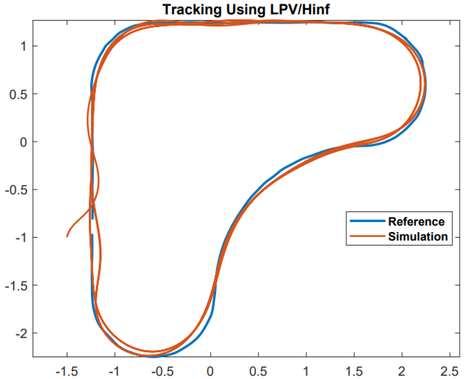
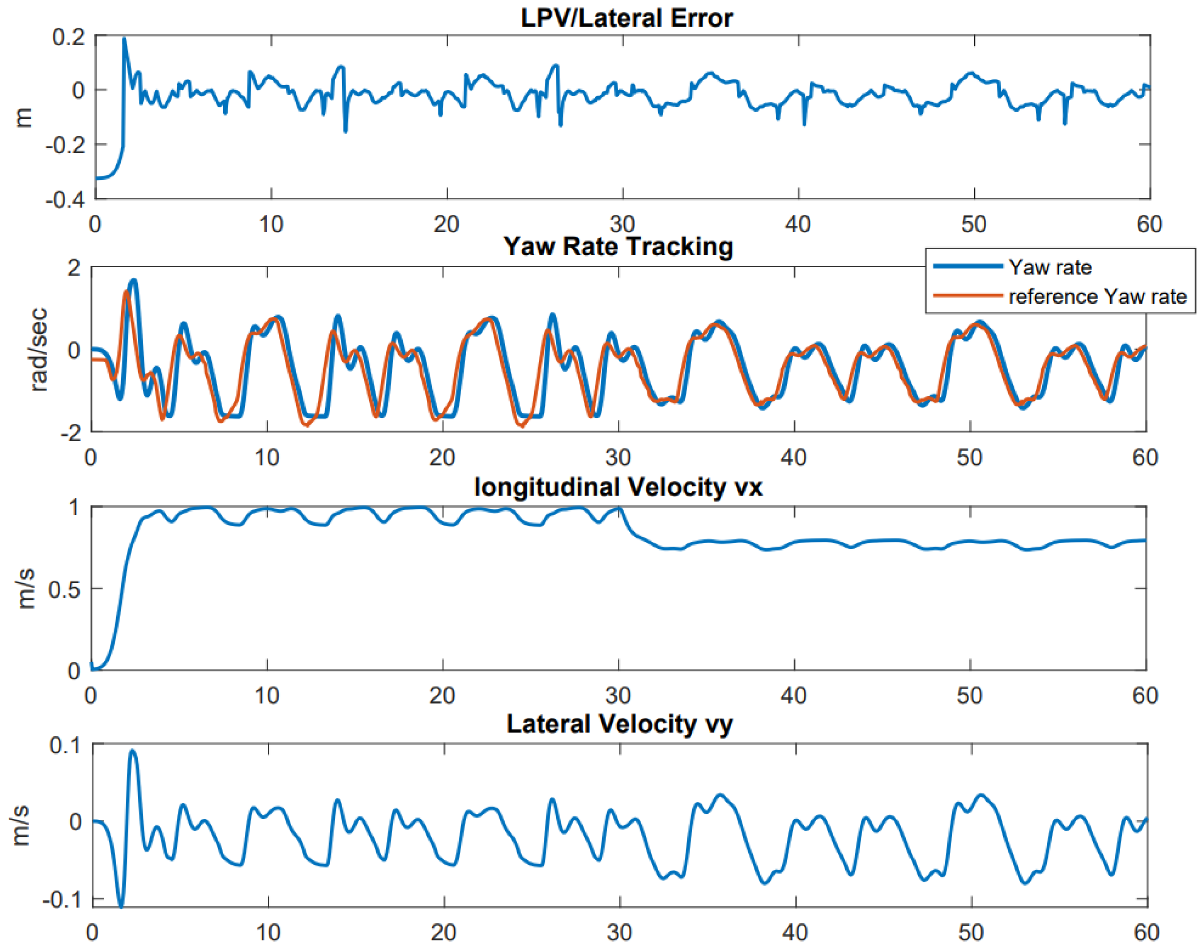
6.2. Simulation of LPV/${\mathcal{H}}_{\infty }$ Controller

As previously mentioned, the reduced polytopic approach is designed with the knowledge that $v_x$ lies within the range of $[0.4,1.6]$ m/s. However, for simulation purposes, the range is assumed to be $[0.8,1]$ m/s. The tracking performance is illustrated in Figure 17, clearly demonstrating the effectiveness of the controller in reducing oscillations during curvature changes. The lateral error mostly falls within the range of 5 cm to 10 cm. The results presented in Figure 18 exhibit the excellent tracking performance of the yaw rate, which closely follows its desired reference.

6.3. Experimental Results of LTI/${\mathcal{H}}_{\infty }$

The designed controller was successfully implemented in real time. The vehicle underwent several rounds of testing with varying $v_x$ values, constrained within the designed range. Experimental tracking results are presented in Figure 19, demonstrating that the vehicle effectively tracks the track with good performance. Figure 20 showcases the states of the vehicle during the experiment, with the yaw rate accurately tracking the generated reference and the lateral error staying below 15 cm.

It is important to note that this controller is specifically designed for $v_x$ limited to 1 m/s, as oscillations and vehicle instability can occur beyond this limit. The controller ensures stability and optimal performance within this velocity range.

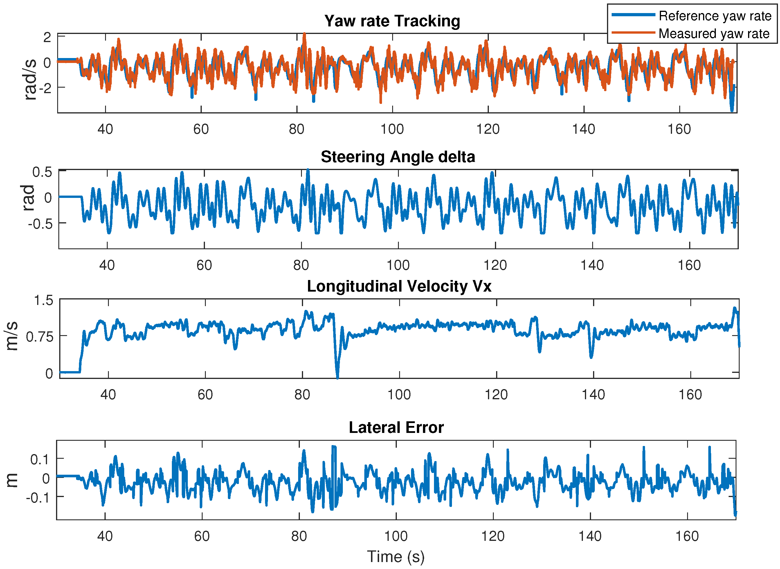
6.4. Experimental Results of LPV/${\mathcal{H}}_{\infty }$

The vehicle completed multiple rounds around the identified trajectory. The longitudinal velocity was controlled using a joystick to maintain $v_x$ within the range of $[0.5,1.3]$ m/s. Figure 21 displays the position of the vehicle relative to the defined reference. It is important to note that the initial conditions of the controller significantly impact its stability and efficiency. The maximum lateral error, as depicted in Figure 22, occurs when the vehicle’s longitudinal speed reaches $v_x=1.5$ m/s. During the second curvature, where the vehicle oscillates three times, the high value of $v_x$ relative to the vehicle’s dimensions leads to this behavior. It is evident that at lower velocities, the tracking performance is improved, with smaller lateral errors observed. This experiment was conducted at various velocities to assess the controller’s performance under different acceleration and deceleration scenarios.

6.5. Experimental Comparison between LTI and Polytopic LPV

In order to provide a rough comparison between the mentioned strategies, a sample of the experiment presented. Figure 23 and Figure 24 illustrate the range of velocity variation, along with the corresponding lateral error. The root mean square error (RMSE) for the lateral error is calculated to be $0.0581$ for the LTI approach and $0.0567$ for the LPV polytope approach. It is observed that the LPV polytope approach performs better in handling larger values of $v_x$ compared to the LTI approach. During the experiments, the LTI controller reached instability at $v_x$ values higher than $1.2$ m/s, indicating the improved performance achieved using the LPV approach.

7. Conclusions

This study presents a comprehensive approach to address the treatment and design of an autonomous vehicles, covering various aspects, from robotics to control, with the aim of enhancing system functionality and performance.

• We introduced the ROS2 environment, achieved through the design and development of a versatile architecture that breaks down the vehicle software controller into distinct levels. Each of these levels was addressed and adjusted independently.
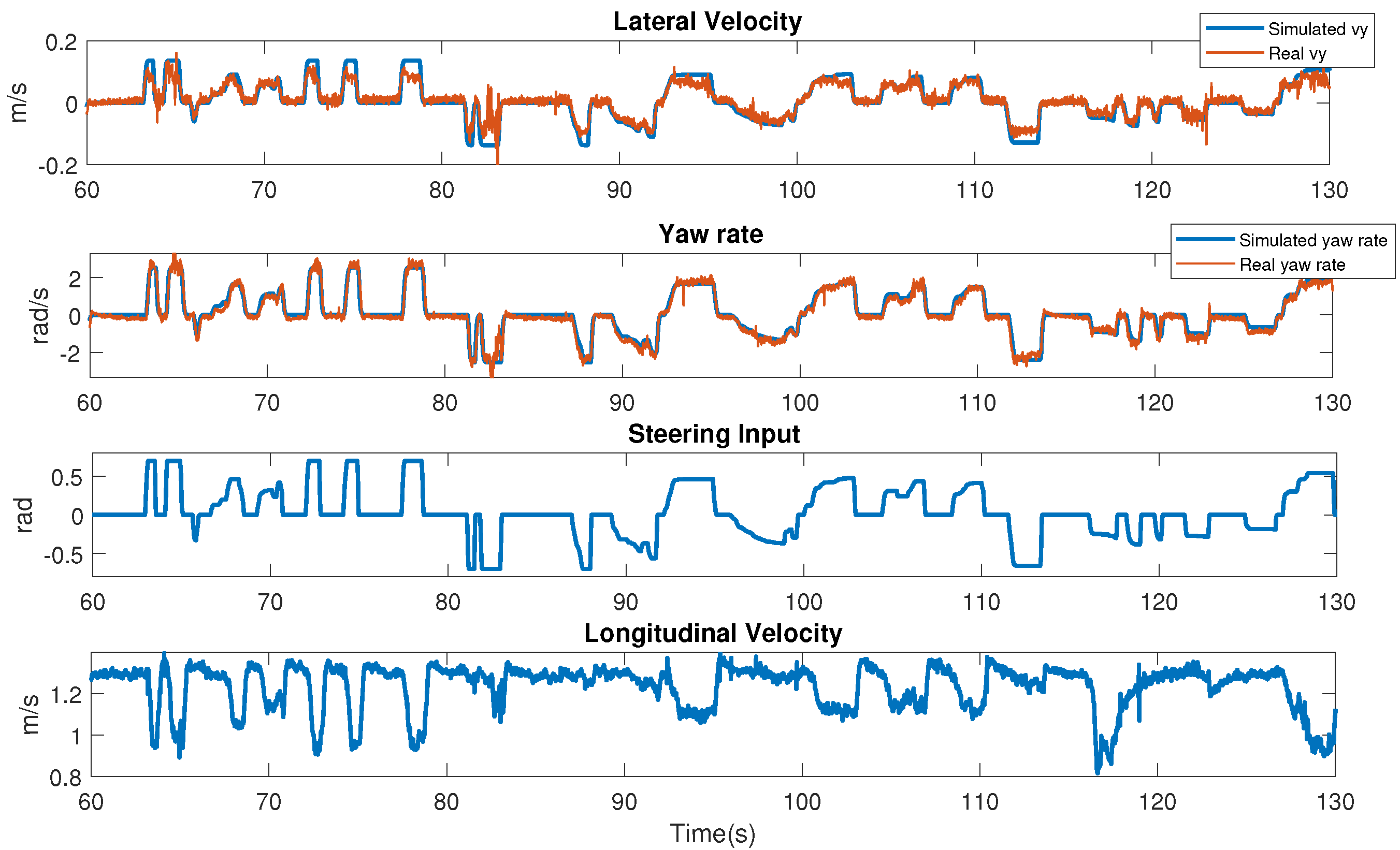
• We introduced a concise discussion of the lateral dynamic model of the system, highlighting the impact of $v_x$ on its linear mode. Additionally, a parameter estimation-based prediction error method was presented, accompanied by realistic outcomes.
• The system is categorized as LTI or LPV depending on the variation of $v_x$. For each scenario, a robust ${\mathcal{H}}_{\infty }$ controller was designed and practically implemented using the previously described ROS2 architecture. In terms of experimental comparison, this study reveals the limitations of the LTI/${\mathcal{H}}_{\infty }$ approach compared to the LPV/${\mathcal{H}}_{\infty }$ approach, particularly when dealing with velocities higher than the designed operating point.

This fundamental architecture has room for enhancement across various dimensions. From a robotics perspective, focusing on localization through onboard sensors can significantly enhance the car’s sensing and perception capabilities. Additionally, the implementation of filters and observers to mitigate measurement noise and enhance sensing reliability is crucial. On a different note, incorporating longitudinal control is essential to manage full vehicle dynamics. Different controllers, like MPC, MFC, and adaptive controllers, for both dynamics can yield improved performance and should be thoroughly tested.

References

- Aria, E.; Olstam, J.; Schwietering, C. Investigation of Automated Vehicle Effects on Driver’s Behavior and Traffic Performance. Transp. Res. Procedia 2016, 15, 761–770. [Google Scholar] [CrossRef]
- Czech, P.; Turoń, K.; Barcik, J. Autonomous vehicles: Basic issues. Zesz. Naukowe. Transp./Politech. Śląska(100) 2018, 100, 15–22. [Google Scholar] [CrossRef]
- Paden, B.; Čáp, M.; Yong, S.Z.; Yershov, D.; Frazzoli, E. A Survey of Motion Planning and Control Techniques for Self-Driving Urban Vehicles. IEEE Trans. Intell. Veh. 2016, 1, 33–55. [Google Scholar] [CrossRef]
- Raviteja, S.; Shanmughasundaram, R. Advanced Driver Assitance System (ADAS). In Proceedings of the Second International Conference on Intelligent Computing and Control Systems (ICICCS), Madurai, India, 14–15 June 2018; pp. 737–740. [Google Scholar] [CrossRef]
- Kılıç, I.; Yazıcı, A.; Yıldız, Ö.; Özçelikors, M.; Ondoğan, A. Intelligent adaptive cruise control system design and implementation. In Proceedings of the 10th System of Systems Engineering Conference (SoSE), San Antonio, TX, USA, 17–20 May 2015; pp. 232–237. [Google Scholar] [CrossRef]
- Liu, W.; Hua, M.; Deng, Z.; Meng, Z.; Huang, Y.; Hu, C.; Song, S.; Gao, L.; Liu, C.; Shuai, B.; et al. A Systematic Survey of Control Techniques and Applications in Connected and Automated Vehicles. arXiv 2023, arXiv:2303.05665. [Google Scholar] [CrossRef]
- Wang, Z.; Zhou, X.; Wang, J. Extremum-Seeking-Based Adaptive Model-Free Control and Its Application to Automated Vehicle Path Tracking. IEEE/ASME Trans. Mechatron. 2022, 27, 3874–3884. [Google Scholar] [CrossRef]
- PTOLEMUS Consulting Group. 2019. Available online: https://www.ptolemus.com/topics/autonomous-vehicles/ (accessed on 24 June 2023).
- Sayssouk, W.; Atoui, H.; Medero, A.; Sename, O. Design and experimental Validation of an H-infinty Adaptive Cruise Control for a Scaled Car. In Proceedings of the ICMCE—10th International Conference on Mechatronics and Control Engineering (ICMCE 2021), Lisbon, Portugal, 26–28 July 2021. [Google Scholar]
- Kayacan, E. Multiobjective H∞ Control for String Stability of Cooperative Adaptive Cruise Control Systems. IEEE Trans. Intell. Veh. 2017, 2, 52–61. [Google Scholar] [CrossRef]
- Laib, K.; Sename, O.; Dugard, L. String Stable H∞ LPV Cooperative Adaptive Cruise Control with a Variable Time Headway. In Proceedings of the IFAC WC 2020—21st IFAC World Congress, Berlin, Germany, 11–17 July 2020. [Google Scholar]
- Luo, L.; Liu, H.; Li, P.; Wang, H. Model predictive control for adaptive cruise control with multi-objectives: Comfort, fuel-economy, safety and car-following. J. Zhejiang Univ. Sci. A 2010, 11, 191–201. [Google Scholar] [CrossRef]
- Sancar, F.E.; Fidan, B.; Huissoon, J.P.; Waslander, S.L. MPC based collaborative adaptive cruise control with rear end collision avoidance. In Proceedings of the IEEE Intelligent Vehicles Symposium Proceedings, Dearborn, MI, USA, 8–11 June 2014; pp. 516–521. [Google Scholar] [CrossRef]
- Atoui, H.; Sename, O.; Milanés, V.; Molina, J.J.M. LPV-Based Autonomous Vehicle Lateral Controllers: A Comparative Analysis. IEEE Trans. Intell. Transp. Syst. 2021, 23, 13570–13581. [Google Scholar] [CrossRef]
- Kapsalis, D.; Sename, O.; Milanes, V.; Molina, J.M. Design and Experimental Validation of an LPV Pure Pursuit Automatic Steering Controller. IFAC-PapersOnLine 2021, 54, 63–68. [Google Scholar]
- Kosecka, J.; Blasi, R.; Taylor, C.J.; Malik, J. Vision-based lateral control of vehicles. In Proceedings of the Conference on Intelligent Transportation Systems, Boston, MA, USA, 9–12 November 1997; pp. 900–905. [Google Scholar]
- Zhou, X.; Wang, Z.; Wang, J. Popov-H∞ Robust Path-Tracking Control of Autonomous Ground Vehicles With Consideration of Sector-Bounded Kinematic Nonlinearity. J. Dyn. Syst. Meas. Control 2021, 143, 111004. [Google Scholar] [CrossRef]
- Zhao, J.; Li, W.; Hu, C.; Guo, G.; Xie, Z.; Wong, P.K. Robust Gain-Scheduling Path Following Control of Autonomous Vehicles Considering Stochastic Network-Induced Delay. IEEE Trans. Intell. Transp. Syst. 2022, 23, 23324–23333. [Google Scholar] [CrossRef]
- Zhang, H.; Zhang, X.; Wang, J. Robust gain-scheduling energy-to-peak control of vehicle lateral dynamics stabilisation. Veh. Syst. Dyn. 2014, 52, 309–340. [Google Scholar] [CrossRef]
- Brennan, S.; Alleyne, A. Generalized H∞ vehicle control utilizing dimensional analysis. In Proceedings of the 2003 American Control Conference, Denver, CO, USA, 4–6 June 2003; pp. 3774–3780. [Google Scholar] [CrossRef]
- Alcalá, E.; Puig, V.; Quevedo, J. LPV-MPC Control for Autonomous Vehicles. IFAC Pap. 2019, 52, 106–113. [Google Scholar] [CrossRef]
- Menezes Morato, M.; Normey-Rico, J.; Sename, O. Model Predictive Control Design for Linear Parameter Varying Systems: A Survey. Annu. Rev. Control 2020, 49, 64–80. [Google Scholar] [CrossRef]
- Alcalá, E.; Puig, V.; Quevedo, J.; Rosolia, U. Autonomous racing using Linear Parameter Varying-Model Predictive Control (LPV-MPC). Control Eng. Pract. 2020, 95, 104270. [Google Scholar] [CrossRef]
- Ao, D.; Huang, W.; Wong, P.K.; Li, J. Robust Backstepping Super-Twisting Sliding Mode Control for Autonomous Vehicle Path Following. IEEE Access 2021, 9, 123165–123177. [Google Scholar] [CrossRef]
- Tagne, G.; Talj, R.; Charara, A. Higher-Order Sliding Mode Control for Lateral Dynamics of Autonomous Vehicles, with Experimental Validation. In Proceedings of the IEEE Intelligent Vehicles Symposium, Proceedings, Gold Coast City, Australia, 23 June 2013; pp. 678–683. [Google Scholar] [CrossRef]
- Alberri, M.; Hegazy, S.; Badra, M.; Nasr, M.; Shehata, O.M.; Morgan, E.I. Generic ROS-based Architecture for Heterogeneous Multi-Autonomous Systems Development. In Proceedings of the 2018 IEEE International Conference on Vehicular Electronics and Safety (ICVES), Madrid, Spain, 12–14 September 2018; pp. 1–6. [Google Scholar] [CrossRef]
- Reke, M.P.; Schulte-Tigges, D.; Schiffer, J.; Ferrein, S.; Walter, A.; Matheis, T.D. A Self-Driving Car Architecture in ROS2. In Proceedings of the 2020 International SAUPEC/RobMech/PRASA Conference, Cape Town, South Africa, 29–31 January 2020. [Google Scholar]
- Atoui, H.; Sename, O.; Milanés, V.; Martinez, J.J. Intelligent Control Switching for Autonomous Vehicles based on Reinforcement Learning. In Proceedings of the 2022 IEEE Intelligent Vehicles Symposium (IV), Aachen, Germany, 4–9 June 2022. [Google Scholar]
- Medero, A.; Morato, M.M.; Puig, V.; Sename, O. MPC-based optimal parameter scheduling of LPV controllers: Application to Lateral ADAS Control. In Proceedings of the 2022 30th Mediterranean Conference on Control and Automation (MED), Vouliagmeni, Greece, 28 June 2022–1 July 2022. [Google Scholar]
- Chen, G.; Zhao, X.; Gao, Z.; Hua, M. Dynamic Drifting Control for General Path Tracking of Autonomous Vehicles. IEEE Trans. Intell. Veh. 2023, 8, 2527–2537. [Google Scholar] [CrossRef]
- Atoui, H.; Sename, O.; Alcala, E.; Puig, V. Parameter Varying Approach for a Combined (Kinematic + Dynamic) Model of Autonomous Vehicles. IFAC-PapersOnLine 2020, 53, 15071–15076. [Google Scholar] [CrossRef]
- Bamieh, B.; Giarre, L. Identification of linear parameter varying models. In Proceedings of the 38th IEEE Conference on Decision and Control (Cat. No.99CH36304), Phoenix, AZ, USA, 7–10 December 1999; pp. 1505–1510. [Google Scholar] [CrossRef]
- Ho Duc, D. Some Results on Closed-Loop Identification of Quadcopters; Linköping University Electronic Press: Linköping, Sweden, 2018. [Google Scholar] [CrossRef]
- Dominguez, S.; Ali, A.; Garcia, G.; Martinet, P. Comparison of lateral controllers for autonomous vehicle: Experimental results. In Proceedings of the 2016 IEEE 19th International Conference on Intelligent Transportation Systems (ITSC), Janeiro, Brazil, 1–4 November 2016; pp. 1418–1423. [Google Scholar]