1. Introduction
With a rapidly expanding population and obvious climate change, conventional agriculture has been undergoing a profound transformation for several years. Multiple factors, such as low irrigation of crops, depletion of various fossil resources, soil degradation, and a shortage of labor, are leading to a deep change in conventional agricultural methods and a shift towards agriculture 4.0 [
1]. Despite the unfavorable context, we must be able to produce enough food to properly feed the whole population. On the other hand, these changes increase the economic risks for farms with limited means for dealing with these changes. As a result, through their scientific research, the academic and industrial worlds are major players in providing innovative technological solutions. The main challenge is, thus, to reduce economic risks and increase production while ensuring acceptable working conditions for farmers. Of all of the research around autonomous vehicles, the “Navigation” domain opens up interesting perspectives in the field of autonomous agricultural robotics and, more specifically, the contribution to the overall control of such vehicles. The need to better understand, measure, and work with nature relies on advanced methods and tools with dedicated equipment. Today, autonomous agricultural robots are a key element in providing a real solution. On the other hand, the development of lighter robots than conventional machines (i.e., tractors with their specific tools or equipment for spraying or harvesting) is flourishing in order to mitigate problems related to soil compaction and to access fields that are not suitable for heavy machinery (such as sloping vineyards or lands affected by wet conditions) [
2]. In this context, this paper deals with the automation of small off-road agricultural vehicles by providing an innovative robust lateral control architecture for smooth off-road vehicle guidance.
1.1. Objectives and Related Work
In general, the lateral guidance of an autonomous vehicle consists of controlling the lateral position and heading of the vehicle around a given reference trajectory. Many different control methods have been proposed in the literature. The main results were grouped in the study proposed by [
3]. This work illustrated the main approaches used in the literature and the advantages and drawbacks of each method by comparing them. Among the various proposed algorithms, two categories stand out: the so-called “geometric” approach and the dynamic approach.
The geometric approach is the most widely used. It is based on the principle of calculating the steering angle to be applied to a vehicle’s wheels to follow a path defined by a set of points based on the Ackerman principle [
4]. The Follow the Carrot (FC) [
5] and the Pure Pursuit (PP) algorithms [
6] are used very often. These approaches provide simplicity of implementation and a low number of parameters to be adjusted. Moreover, no dynamic models are necessary to represent the vehicle, which greatly simplifies their development. However, the tracking performance deteriorates when the vehicle’s lateral dynamics are solicited—for example, with high-speed profiles, which can impair dynamic performance and/or make the system unstable.
On the other hand, the dynamic approach is based on a vehicle model that allows the explicit calculation of trajectory tracking errors as a function of a vehicle’s dynamics and its parameters. This approach allows the implementation of a more advanced control architecture based on modern synthesis methods, such as, the optimal linear quadratic regulator (LQR) approach [
7], the model predictive control (MPC) approach [
8], robust
approach [
9], or the sliding-mode control (SMC) approach [
10]. An example of an application using this type of dynamic approach was proposed by [
11], where the guidance architecture used a state feedback control that was calculated from the resolution of different linear matrix inequalities (LMIs), which made the approach robust but conservative. The advantage of this type of approach lies in obtaining a controller whose performance can be optimized with respect to the desired performance, thus greatly improving the vehicle’s behavior in high-speed maneuvers. The difficulty, however, lies in the implementation and complexity of the algorithm, since the measurements must be provided as necessary inputs for computing the control output.
However, both of these approaches are mostly applied in on-road conditions where the lateral slip is low [
8,
9,
11]. In the context of deformable soils, this assumption is no longer respected and, consequently, requires the development of a control strategy that takes this phenomenon into account. Different studies have been carried out to improve the guidance of vehicles on deformable ground [
12,
13,
14,
15]. However, the proposed methods simplified the ground’s nature by neglecting the soft soil properties or were applied to trajectories that did not require significant lateral dynamics (for example, straight-line trajectory tracking). More recent works [
16,
17] based on robust sliding-mode control approaches showed real-time implementations that were limited by the fact that the actuator switched at a very high frequency.
This paper is dedicated to the development of a robust lateral guidance strategy for autonomous off-road vehicles. To the best of the authors’ knowledge, the study reported in this work is novel in proposing a robust uncertain- and variant-parameter lateral control architecture that addresses the problem of soft ground by combining both geometric and dynamic approaches to create a whole control architecture.
1.2. Paper Contributions and Organization
In addition to the implementation of the overall robust lateral guidance architecture, this paper includes multifold contributions, which are summarized as follows:
A global guidance architecture based on an original combination of geometric and dynamic algorithms.
A modification of the Pure Pursuit algorithm that now computes the lateral error based on a dynamic parameter related to the look-ahead distance.
Robustness improvements that were achieved by incorporating uncertainties and time-varying parameters in a grid-based LPV control synthesis.
The use of a dedicated off-road vehicle simulator that takes deformable soils into account for the validation of the proposed algorithms.
A real-time integration and validation of the proposed control architecture on a vehicle prototype.
Therefore, this paper is organized as follows:
Section 2 presents the off-road vehicle model, which includes the wheel–ground interaction for soft soils. The lateral guidance problem and the modified Pure Pursuit algorithm are presented in
Section 3. The robust grid-based LPV control approach is given in
Section 4. The
control synthesis is provided in
Section 5. Finally, the simulation results are presented in
Section 6, followed by those of the real-time implementation, which are given in
Section 7.
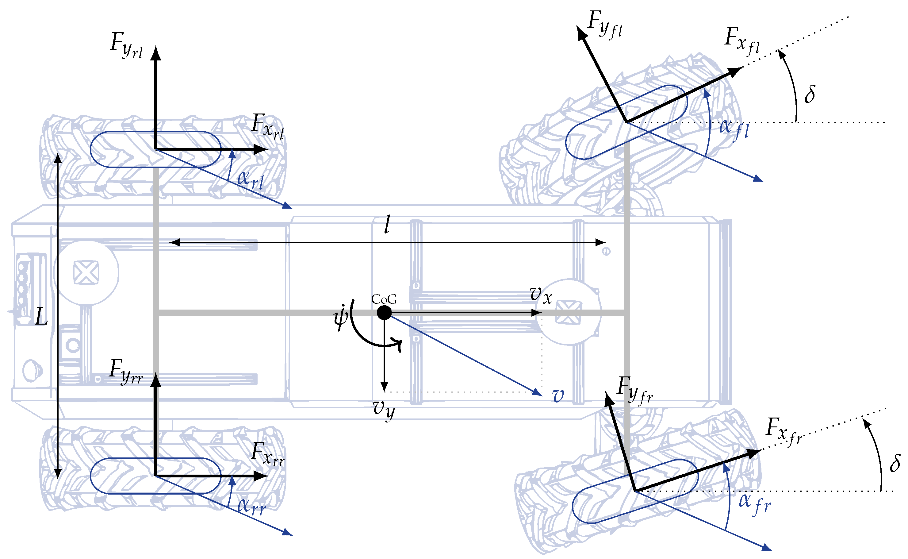
2. Off-Road Vehicle Modeling
To solve autonomous off-road vehicle guidance problems, a nonlinear 7-DOF model is commonly used in the literature [
18]. The associated dynamics are given by the state vector
, which are, respectively, the longitudinal and lateral velocities, the yaw rate, and the angular wheel rate of the
ith wheel, with
.
Figure 1 reports a schematic representation of such a model, and
Table 1 gives the meanings of the different symbols that are used.
Some classical assumptions are also employed:
Pitch, roll, and vertical motions are neglected.
Aerodynamic drag force is considered null due to the low speeds employed in this application.
The front steering angle has a low range of variation and is considered equal for both the left and right wheels.
Let us remark that the particularity of ground vehicles addresses the wheel–soil interaction problem, where soil deformation highly affects a vehicle’s behavior [
19].
This specificity is represented through the longitudinal (
) and lateral (
) forces and will be discussed in more detail in
Section 2.3. Moreover, the longitudinal and lateral dynamics are expressed as presented in the following subsections.
2.1. Longitudinal Vehicle Model
The longitudinal vehicle dynamics represent one of the most important factors for ground vehicles. Converting wheel power into vehicle motion is strongly related to the ability to generate sufficient traction between the wheels and the ground. In this purpose, the connection is described by the following torque balance equation, which is applied for each
ith wheel:
where
J is the wheel inertia,
r is the wheel’s effective radius, and
and
are, respectively, the driving and friction torque of the wheel. The equation of the longitudinal dynamics expressed at the center of gravity (CoG) is given by [
18]:
where
is the longitudinal tire force generated at the
ith wheel and is transformed into the vehicle frame.
2.2. Lateral Vehicle Model
The lateral vehicle model is represented through the lateral dynamic equation and is expressed at the CoG by [
18]:
where
is the lateral force applied at the
ith wheel and is transformed into the vehicle frame. The yaw equation is then given by:
where
denotes the vehicle’s inertia along the z-axis, and
and
are, respectively, the lateral forces applied at the front and rear
ith wheels and are transformed into the vehicle frame. In addition,
and
are, respectively, the distance between the front and rear axles and the CoG.
2.3. Soft Wheel–Soil Interaction Model
For ground vehicles, wheel–soil interaction phenomena have a significant impact on a vehicle’s dynamics, since the soil deformation greatly affects traction and wheel grip [
19]. In classic on-road contexts, several model types have been proposed in the literature [
20,
21,
22]. However, these models are not able to capture the complex off-road phenomena. Therefore, specific off-road tire models are required. As a common approach, the predicted off-road tire forces are provided according to the Bekker–Wong theory [
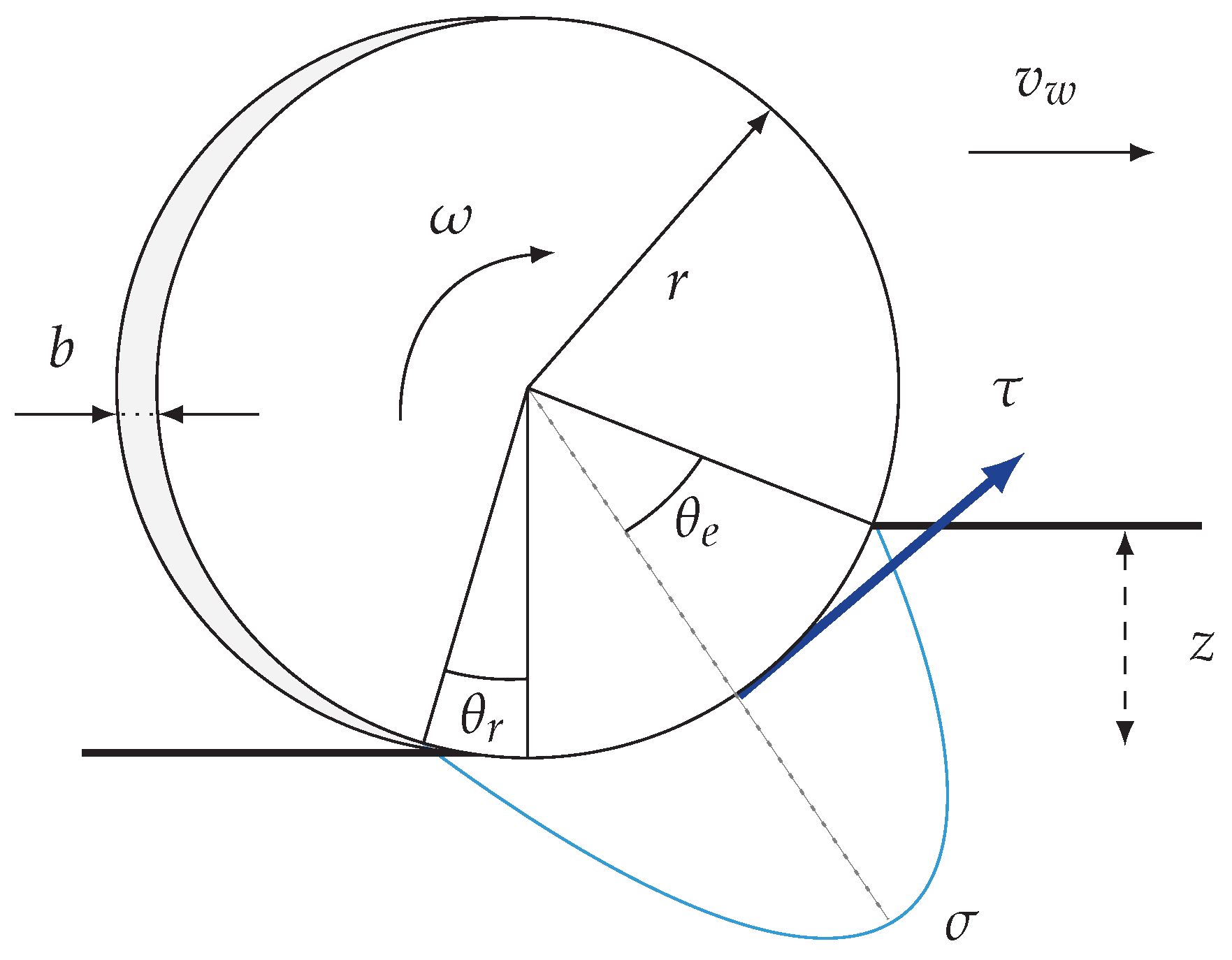
23]. Considering the mathematical framework provided in [
24], the longitudinal and lateral tire forces can be expressed as follows:
where
b is the wheel width,
is the shear stress acting at the wheel contact patch,
is the normal stress,
c is the soil cohesion coefficient,
is the angle of internal friction of the soil,
is the lateral shear displacement,
is the lateral shear deformation modulus, and
are, respectively, the entry and exit angles given by the soil–wheel contact, as shown in
Figure 2. The interaction at the contact between the wheel and the ground exerts a vertical pressure, which leads to the sinkage (
z) of the wheel into the ground, thus affecting the overall tire forces
and
.
Consequently, the soil acts as an additional resistive force that introduces a significant wheel slip and lateral slip. These relevant phenomena are then introduced into (
2) and (
3), thus affecting the dynamic behavior of the whole body, and they are presented in more detail in [
19,
24,
25]. Considering this wheel–soil interaction problem, the proposed control strategy aims to be robust to the uncertainties introduced by the variation in the soil’s nature, as presented in
Section 3.
3. Lateral Guidance Problem
The lateral guidance problem aims to minimize the errors between a vehicle’s position and the desired reference path. In the context of ground vehicles, and especially in agricultural applications, these errors must be minimized to optimize the working area while ensuring the lowest possible field coverage [
26]. For this purpose, the overall lateral guidance strategy is developed as follows.
3.1. Problem Formulation
By considering the simplified bicycle vehicle model [
4], the main goal of the lateral guidance problem is to minimize the lateral and orientation errors (
and
) between the CoG and the reference path, as shown in
Figure 3. The lateral error can be expressed in the global frame (
X,
Y) as [
4]:
where
and
are, respectively, the coordinates of the vehicle’s position and the reference path points’ coordinates, and
is the desired yaw angle.
The heading error is provided by
where
is the orientation of the vehicle’s CoG in the global coordinate system.
3.2. Control Objectives and Desired Performance
The lateral guidance objectives are specified by considering path tracking at different longitudinal speeds of the vehicle. Since navigation on deformable soil leads to exogenous disturbances that can greatly affect the tracking performance, the vehicle guidance must be robust. As a result, the closed-loop performance is then stated as follows:
A lateral error lower than 20 cm.
The trajectory tracking must be performed for longitudinal speeds between 1 and 15 km/h.
Overshoots around the reference path must be less than 40 cm.
These specifications were established in accordance with the intended applications, whose validation was carried out by T&S Group (industrial partner) in view of its experience in this field. Note that 15 km/h is considered a high speed for agricultural applications.
3.3. A Combined Geometric–Dynamic Lateral Guidance Approach
In order to track the coordinates of the reference points and the orientation of the trajectory, the tracking algorithm provides the steering angle
to be applied to the wheels. To solve this problem, a combined lateral guidance approach is proposed. It is based on combining a geometric algorithm with a controller (synthesized by using a dynamic model) that calculates and minimizes the lateral error. The proposed control architecture is then provided in
Figure 4 and was designed to simplify the integration of the algorithms for real-time implementations. Given the variations caused by the nature of the ground and the longitudinal speed of the vehicle, a purely geometric approach cannot be applied. In this way, a robust controller
is associated with the overall guidance architecture, as seen in
Figure 4, and the development thereof is described in
Section 4.
3.4. Modified Pure Pursuit Algorithm (Geometric Approach)
The geometric algorithm used in this paper is based on the Pure Pursuit (PP) algorithm described in [
6]. It consists of a simple geometric equation that calculates a “virtual” circle of curvature designated by the radius
R from the center of the rear axle to the target point (
) on the path ahead of the vehicle, as shown in
Figure 5. The target point is determined from the look-ahead distance
, and the desired steering angle
is obtained from the angle
, which defines the vehicle’s orientation relative to the look-ahead distance
.
This approach is modified here to improve the tracking performance according to the following propositions:
Local trajectory generation: This modification defines a sliding window based on a certain number of points chosen among the total number of points constituting the global trajectory in the local navigation frame. It reduces the computational load and allows the management of trajectories with intersections.
Lateral error computation: The target point is projected into the vehicle frame to compute the lateral error.
Adapted look-ahead distance: The parameter
is adapted according to the vehicle’s longitudinal speed with the following equation:
with
and
being constants and
.
Steering angle computation: The required steering angle is calculated from the lateral error and not from the Ackerman angles. A controller is then employed to provide the steering angle in order to cancel the lateral error between the vehicle and the reference trajectory.
As mentioned before, a pure geometric algorithm cannot minimize the lateral errors, as the soil dynamically affects the vehicle’s behavior. The dynamic compensation is, thus, obtained by adding a robust controller, as presented in the next section.
4. A Robust Quasi-Grid-Based LPV- Control Approach
The proposed approach is based on an LPV (linear parameter-varying) representation. This is generally used when some parameters vary over time. Such representations have several advantages, e.g., they take nonlinearities into account and use the synthesis tools of LTI models. They allow the consideration of unmeasured variables as uncertainties to reduce their impacts on the closed-loop behavior when they are involved in the model. Consequently, a synthesis model is established to allow the design of a robust controller that is capable of ensuring closed-loop performance regardless of the value of the uncertainty contained in a bounded range.
4.1. Vehicle Synthesis Model
The lateral synthesis model developed in this section aims to describe the lateral behavior of the vehicle with sufficient accuracy while reducing its complexity.
This model is obtained from Equations (1)–(5b) and is expressed through the following state-space representation:
where
and
are, respectively, the front and rear center-of-gravity distances,
is the vehicle’s moment of inertia around the vertical axis,
m is the total mass of the vehicle, and
and
are, respectively, the front and the rear cornering stiffnesses obtained by considering the Adapted Burckhardt Tire Model (ABTM), as developed in [
27]. Due to the complexity of Equations (
5a) and (
5b), a straightforward interaction model for control design cannot be obtained. An equivalent cornering stiffness
for each wheel can then be addressed by identifying the ABTM parameters and linearizing the model as follows:
The coefficient
was derived through an identification procedure proposed by the authors in another article [
27]. This procedure encompasses four steps:
Collecting data that correspond to different deformable soils that were studied by using a dedicated simulation tool.
Adapting the mathematical structure of the interaction model (ABTM).
Identifying new parameters.
Determining the range of variation in stiffness of around different operating points.
By using model (11), it is possible to establish a set of values that include a nominal value and its deviation within a bounded range, where is the identified model parameter for a given soft soil and is the lateral slip operating point.
On the other hand, a steering actuator defined by a linear cylinder is considered and is given by the following transfer function between the linear position
and the steering angle
:
where
is the static gain,
is the natural frequency, and
is the damping ratio. The transfer function parameters were obtained from an identification procedure by using the harmonic response of an actuator with real recorded data.
Thereby, the model (
8) expresses the uncertainties through the coefficients
and
, which correspond to variations in the nature of the ground. The varying parameter is the vehicle’s longitudinal velocity
, which renders the overall model as an uncertain LPV system.
4.2. Quasi-Grid-Based LPV Approach
The grid-based LPV approach leverages an interpolation network of linearized LTI models around different operating points [
9]. This approach is commonly used when the parametric dependence of the model is nonlinear. The varying parameters are then gridded and selected with a
N points, as shown in
Figure 6. Note that the interpolation between each model can be linear or nonlinear.
where
p is the number of variant parameters and
and
are, respectively, the minimum and the maximum values of the considered variant parameter.
Thus, the grid-based LPV model representation is given by a linear interpolation between two points of the state-space matrices as follows:
with
and with
being given by:
By using this modeling approach, a
K controller is independently synthesized with each linear model defined in the grid and is linearly interpolated as follows:
where
and
are as defined in (
13). Despite its simplicity, it must be emphasized that the local stability of each controller does not guarantee the global stability of the closed-loop system. A stability assessment could be conducted according to the work proposed by [
28,
29]. The stability problem can be addressed by using a Lyapunov candidate function that depends on the varying parameter
. However, as shown in [
9], a large number of models and, consequently, controllers must be designed. This causes conservatism and, therefore, degrades the performance in the closed loop. On the other hand, the model (
8) is not only parameter-variant, but also uncertain with respect to the soil’s nature through the
parameters. However, an LPV model cannot be established, since the nonlinearity is not measurable. Thus, this solution cannot be considered.
Consequently, the proposed method uses the grid-based LPV approach that describes the time-varying parameter to
but differs by performing the controller’s synthesis separately by using a
approach to be robust to the
uncertainties, as described in
Section 5.
5. Grid-Based LPV- Control Design
In this section, the controller synthesis is addressed by using an
mixed-sensitivity approach [
30], where the general scheme is given in
Figure 7.
The figure presents a control block diagram in which
is the controller and
is the plant given by the actuator model (
10) that is added to the vehicle model dynamics (
8). The controller output
rejects the lateral error
, where
is the lateral reference position and
y is the current lateral position of the vehicle. Therefore, the main objective of the
control is to minimize the
-induced gain from the external input
to the controlled output
by solving the following minimization problem:
where
represents the attenuation gain. Moreover, the mixed-sensitivity approach amounts to searching for a controller
that ensures the internal stability of the closed loop and satisfies the following constraints [
30]:
where
and
are weighting functions that specify a trade-off between the limitations of the tracking and actuator performance, with
being the sensitivity function of the output
y to the reference
.
5.1. Weighting Functions
The weighting functions offer the possibility of setting up the closed-loop performance. By considering the actuator–vehicle model (
8)–(
10), the weighting functions
,
are defined according to the work proposed by [
31]. Consequently, the tracking weighting function is given by
where
,
is the break frequency,
is the maximum permissible static error, and
k is the transfer function order. Similarly, the actuator weighting function is given by
where
,
is the break frequency,
is the maximum permissible static error, and
k is the transfer function order. Note that the weighting functions’ parameter values will be discussed in the next section.
5.2. Grid-Based LPV- Control Synthesis
Referring to the guidance problem mentioned in
Section 3 and considering the uncertain grid-based LPV model described in
Section 4.2, the uncertain parameter
is fixed at its nominal value of 10,000 N and has a standard deviation of ±50%. This was determined by using the computation procedure described in
Section 4.1. The varying parameter
is considered to be bounded as follows:
and the grid is represented by two LTI models (
8) such that the quality of the nonlinear model’s approximation can be assessed through the analysis provided by
Figure 8.
In order to validate the model’s approximation with two vertices, the computation error between the output
of the nonlinear model (
3) and the output
of the model expressed by (
12) is evaluated. The error between these two quantities assesses the quality of the grid-based model, which is evaluated under the assumption that the maximum steering angles are bounded between
°. The error between the two models is then quantified by calculating the root mean square error (RMSE), whose value is
The obtained results indicate that the approximation of the grid-based model can then be specified with only two vertices as follows:
Therefore, two controllers are designed (one at each vertex), the combination of which is achieved linearly via Equation (
13). The values of the weighting functions selected for each controller are provided in
Table 2. The
synthesis result of each controller is then given by the performance index
, as presented in
Table 3.
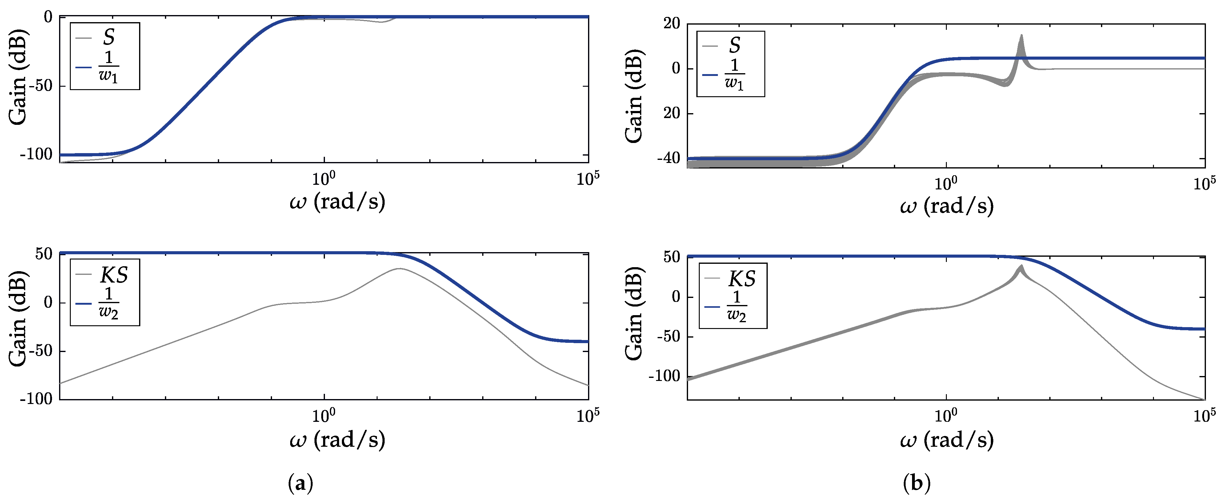
5.3. Frequency Domain Analysis of Synthesis Results
The controller’s synthesis requirements can be verified with the performance index
, as well as with the frequency domain. The results are provided in
Figure 9, where the sensitivity functions are compared to the weight functions designed in
Section 5.1 for each model in the grid.
As the sensitivity functions S are under the weight for both vertices, the demanded tracking error is achieved. On the other hand, the sensitivity functions are compared with the weight . Here, the control input shows that each controller respects the demanding limitations regarding noise sensitivity. Based on these overall results, the global control architecture can then be proposed and applied to the lateral guidance problem.
6. Simulation Results and Analysis of the Developed and Tuned Robust Lateral Control Architecture
This section is devoted to describing a simulation of the proposed lateral control architecture for off-road vehicle guidance based on the ProjectChrono simulator [
32]. The choice of this simulator was due to its ability to model deformable ground, unlike other popular vehicle simulators, such as Car-Maker [
33], Carla, Adams, etc. It uses an accurate wheel–ground contact model [
34] to characterize all off-road vehicle dynamics [
35]. The simulations were performed in discrete time with a sampling time of
ms.
6.1. Global Lateral Vehicle Guidance Architecture
The developed robust lateral control architecture for the autonomous lateral guidance of the vehicle is presented in
Figure 10.
The global architecture included a number of independently developed components:
The local path planner was designed to calculate a lateral error to be minimized.
A grid-based LPV controller made the guidance robust to the vehicle’s longitudinal speed and variations in the soil’s nature.
An extended Kalman filter state estimator, as developed in [
36], ensured the accuracy of the vehicle’s location and attitude.
Moreover, the simulated vehicle was designed according to an off-road prototype developed in collaboration between IRIMAS and T&S Group, as shown in
Figure 11.
In addition, the vehicle parameters and the PP parameters are given in
Table A1.
6.2. Simulation Results
Among the multiple simulations that were performed to validate the proposed robust lateral guidance architecture (see
Figure 10), those that were chosen are discussed hereafter. Two cases were considered to show the robustness regarding the speed and the variations in the soil’s nature.
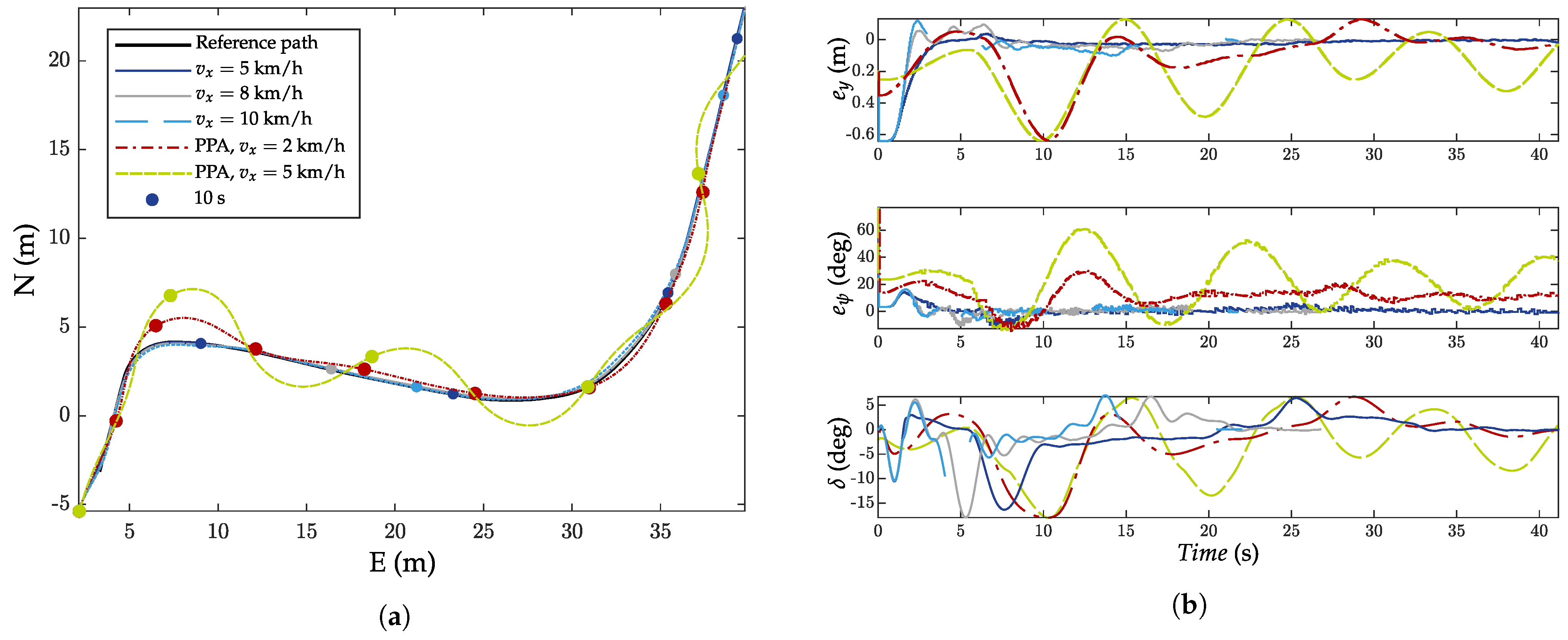
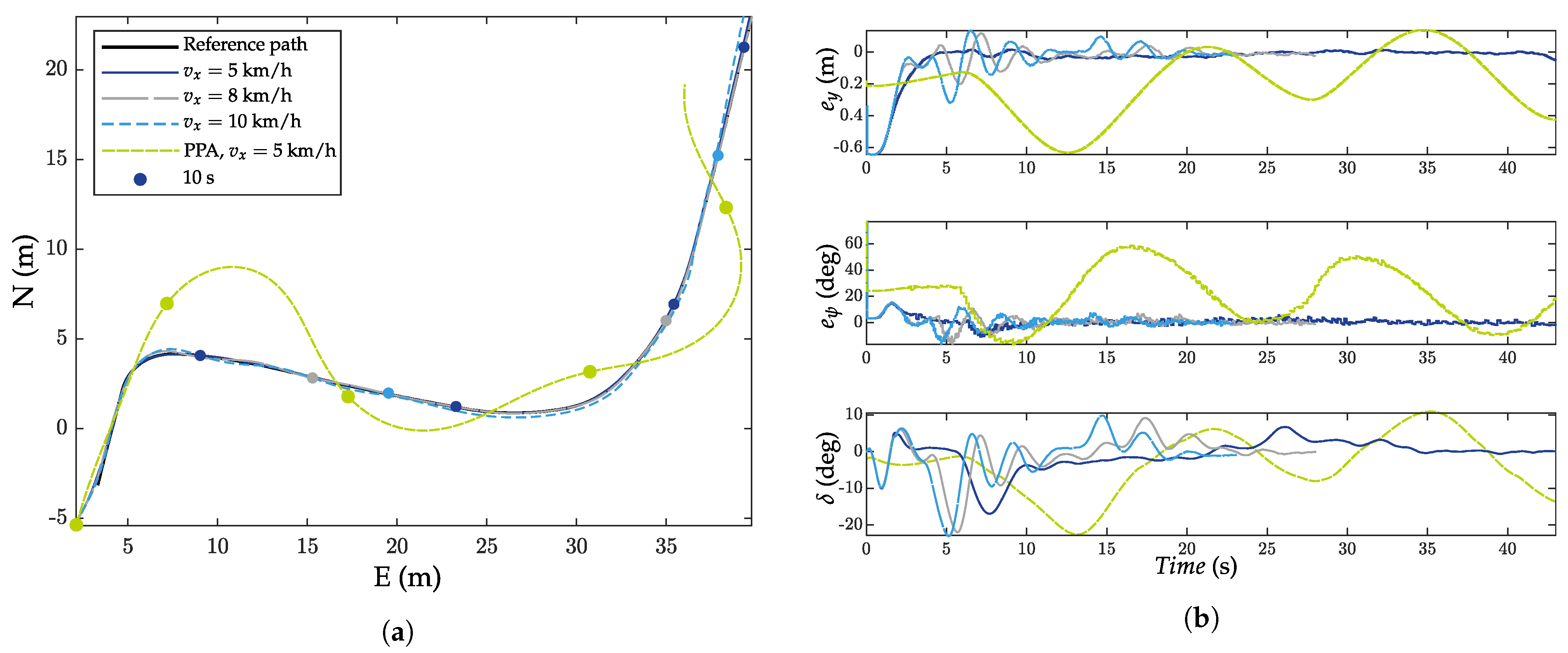
The first case (
Figure 12) considered the lateral guidance of an autonomous vehicle for different longitudinal speeds on rigid soil. The adhesion was represented by dry weather conditions.
The second (
Figure 13) case showed the lateral guidance of an autonomous vehicle with different longitudinal speeds on deformable ground. The proposed test considered sandy soil, which is the worst-case situation with respect to soil deformation.
From a general perspective, the guidance performance that was obtained on rigid soil remained relatively consistent regardless of the longitudinal speed while within the specified range of variations.
Figure 12b illustrates that the lateral error, heading error, and steering angle exhibited similar magnitudes. Furthermore, the root mean square (RMS) of the lateral error, which was represented by the performance indicator in
Table 4, showed very close values for the three different longitudinal speeds achieved with the robust control strategy.
For the purpose of comparison, the proposed method was evaluated against a geometric controller called the Pure Pursuit algorithm (PPA). This type of controller is typically employed for vehicles operating at low speeds, as mentioned in [
9,
37].
Figure 12a and
Figure 13a clearly demonstrate that the trajectory tracking was weaker compared to that of the robust method, and the overall behavior of the vehicle showed oscillatory tendencies. This phenomenon arises when the dynamics of the vehicle, particularly those related to the steering actuator, can no longer be ignored, as was the case in this study. Consequently, it became impossible to impose any performance criteria or constraints during the controller synthesis to mitigate this behavior.
On the other hand, the results displayed in
Figure 13 show the lateral vehicle guidance alongside the previously mentioned path while running on sandy soil. The lateral error, heading error, and applied steering angle for each longitudinal speed are also presented. The obtained results successfully highlight the identical global path tracking performance on deformable ground with the robust control strategy, and the lateral tracking errors are given in
Table 5. However, a more significant overshoot can be noticed during the first turn of the trajectory, as depicted in
Figure 13a. This behavior can be explained by the greater amount of lateral drift caused by the extremely deformable and non-cohesive characteristics of the soil.
In conclusion, the simulated tests on rigid and deformable ground presented in this section demonstrated the strong lateral guiding performance. As a result, a real-time implementation of the global control architecture was realized and tested with an experimental vehicle, as described in
Section 7.
7. Real-Time Implementation
In this section, different experimental results are presented to point out the efficiency of the proposed global control structure in real time. As the prototype vehicle was equipped with a number of sensors (GNSS, IMU, Lidar, etc.) and actuators (linear cylinder, electric motor), it was intended to make navigation autonomous and safe in rough environments. The different elements of the overall control architecture were integrated into STM32 microcontrollers, whose main functions were embedded in the C programming language. In addition, the vehicle’s longitudinal speed was regulated by a robust controller together with the lateral guidance.
Therefore, two different tests were set to validate the proposed guidance algorithm in real time.
The first test (
Figure 14), which was conducted on a rigid surface at different speeds and values of tire pressure, simulated variations in tire stiffness and, consequently, in wheel–soil interaction; the objective was to demonstrate the robustness with respect to uncertainties in the
parameter.
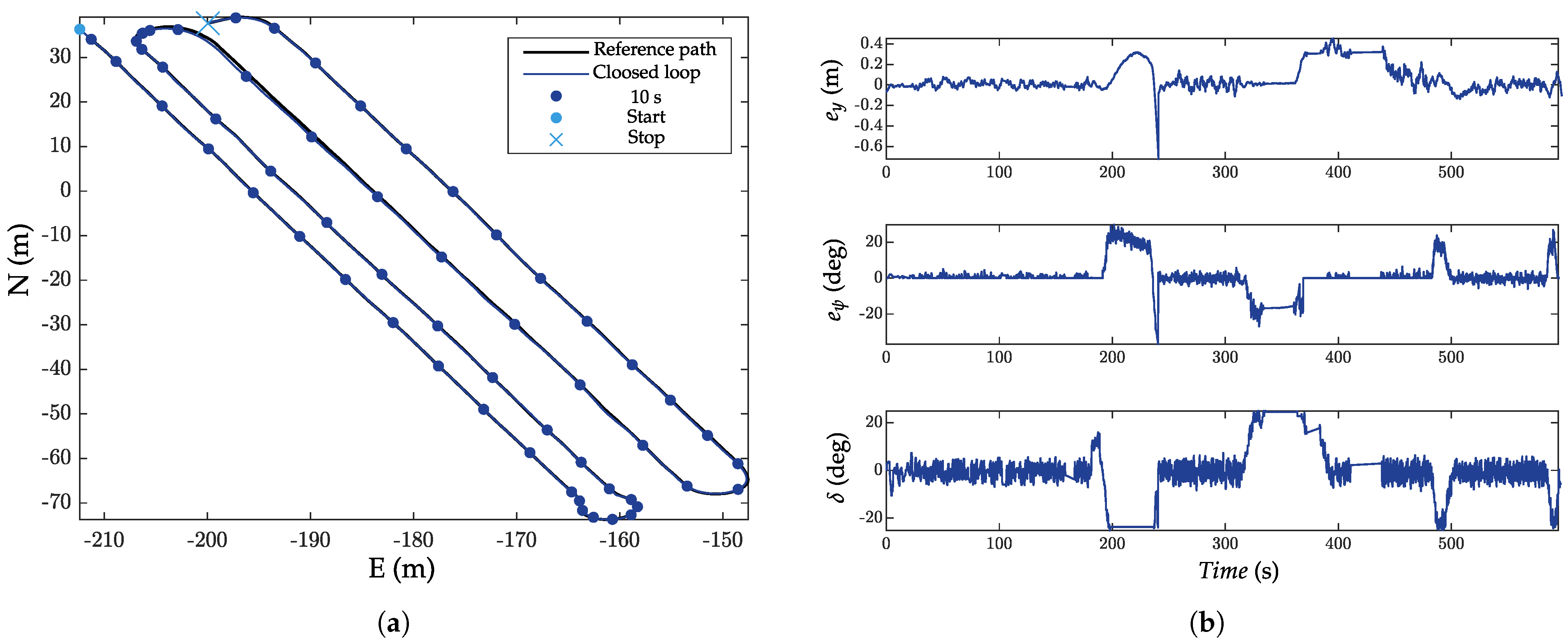
The second experiment was conducted at variable longitudinal speeds on soft ground. A typical agricultural work trajectory (
Figure 15) was proposed and defined with two zones; the work zone, in this case, had straight lines and U-turns. In this scenario, each straight line had a different longitudinal speed, while for the U-turns, the speed was set to a maximum of 1 km/h.
The first test was performed by substituting different deformable soil types with different tire inflation pressures. These tests offered the possibility of easily modifying the parameter in a known and reproducible environment, since the tire pressure could be measured in practice, unlike the nature of the terrain, which could be affected by different types of disturbances. Six tests were realized for three different speeds (i.e., 5, 8, and 10 km/h) and two different inflation pressures (i.e., 0.5 and 0.2 bar).
Note that the tire pressures that were used were particularly low considering the special low-pressure tires used for this type of vehicle. According to
Figure 14b,d,f, the amplitude variations of the lateral error, heading error, and control output were approximately similar. Moreover, the steering angle error was quantified and is given in
Table 6. It can be seen that as the inflation pressure decreased, the lateral error decreased.
Figure 14e clearly shows this phenomenon, since the overshoot during the first turn was greater for the pressure of 0.5 bar than for 0.2 bar. This result is interesting, since it helps one understand the physical relationship between the size of the contact patch and the lateral forces that are generated.
The second test involved an agricultural work trajectory in an orchard (
Figure 16c) whose soil was heterogeneous, i.e., it was composed of both ground and lawn areas. These tests were also realized at longitudinal speeds varying between 1 and 7 km/h.
In the proposed case, each straight line was assigned to a different longitudinal speed, while the speed for U-turns was set to a maximum of 1 km/h. It can be seen that the obtained results ensured fully safe and autonomous navigation along the whole working trajectory. The performance that was obtained in terms of lateral guidance accuracy showed that the uncertainty related to the nature of the ground, as well as the variations in the longitudinal speed, did not degrade the guidance objectives defined in the specifications in
Section 3.2.
8. General Conclusions
This paper addresses the problem of robust lateral guidance in off-road vehicles navigating on deformable grounds that involve variable and uncertain parameters. The paper proposes a global lateral guidance architecture that was validated in a simulation and implemented in a vehicle prototype. The proposed approach combines lateral guidance with a geometric algorithm and a dynamic controller, which provided robustness and simplicity of integration in a real prototype.
The geometric Pure Pursuit algorithm was used to minimize the lateral error at each sample time, followed by a robust controller that took longitudinal speed variations and uncertainties related to wheel–ground interactions into account. The resulting solution with the coupling between the robust control and localization modules constitutes a global control architecture that automates the lateral guidance of off-road vehicles that serve various precision agricultural tasks.
The proposed control architecture was validated in a simulation by using the ProjectChrono environment and was integrated into a prototype. The experimental tests demonstrated the feasibility of the solution, which showed similar guidance performance with respect to the objectives set during the control law synthesis, regardless of the terrain type.
However, it is acknowledged that more complex terrain configurations, such as slopes, banks, and bumps, still need to be addressed to improve the robustness of the proposed control architecture. Additionally, the autonomous guidance of a vehicle while considering an attached or hitched tool is an interesting perspective that should be explored in future research.
Author Contributions
D.V.: Investigation, Methodology, Software, Validation and Writing—original draft; A.V.: Investigation, Methodology, Software, Validation; R.O.: Supervision and Writing—review & editing; M.S.: Project administration, Resources and Supervision; M.B.: Supervision and Writing—review & editing. All authors have read and agreed to the published version of the manuscript.
Funding
This research was funded by Technology and Strategy Group and the French National Association of Research and Technology (ANRT).
Data Availability Statement
Not applicable.
Conflicts of Interest
The authors declare no conflict of interest.
Appendix A
Table A1.
Vehicle and Pure Pursuit parameter values.
Table A1.
Vehicle and Pure Pursuit parameter values.
| Vehicle Parameters | Value (Unit) | Description |
|---|
| l | 1.26 m | Wheelbase: |
| 0.57 m | Front CoG distance |
| 0.69 m | Rear CoG distance |
| L | 0.9 m | Track width |
| m | 440 kg | Vehicle total mass |
| 82.4 kg/m2 | Vehicle moment of inertia |
| h | 0.31 m | CoG height |
| 15 kg | Wheel weight |
| r | 0.30 m | Wheel radius |
| b | 0.203 m | Wheel width |
| 0.99 kg/m2 | Wheel moment of inertia |
| 16 Nm | Nominal motor torque |
| 42 Nm | Maximal motor torque |
| | Maximal steering angle |
| PP-Parameters | Value (Unit) | Description |
| 0.36 s | Look-ahead time gain |
| 0.83 m | Constant look-ahead distance |
| 1.33 m | Minimal look-ahead distance |
| 5 m | Maximal look-ahead distance |
References
- Javaid, M.; Haleem, A.; Singh, R.P.; Suman, R. Enhancing smart farming through the applications of agriculture 4.0 technologies. Int. J. Intell. Netw. 2022, 3, 150–164. [Google Scholar] [CrossRef]
- Santos Valle, S.; Kienzle, J. Agriculture 4.0: Robotique Agricole et Matériel Automatisé au Service D’une Production Agricole Durable; Technical Report; Direction de l’information légale et administrative: Rome, Italia, 2021. [Google Scholar]
- Yao, Q.; Tian, Y.; Wang, Q.; Wang, S. Control strategies on path tracking for autonomous vehicle: State of the art and future challenges. IEEE Access 2020, 8, 161211–161222. [Google Scholar] [CrossRef]
- Rajamani, R. Vehicle Dynamics and Control; Springer Science & Business Media: Berlin/Heidelberg, Germany, 2011. [Google Scholar]
- Wit, J.S. Vector Pursuit Path Tracking for Autonomous Ground Vehicles. Ph.D. Thesis, University of Florida, Gainesville, FL, USA, 2000. [Google Scholar]
- Coulter, R.C. Implementation of the Pure Pursuit Path Tracking Algorithm; Technical Report; Carnegie-Mellon Pittsburgh University, Robotics INST: Pittsburgh, PA, USA, 1992. [Google Scholar]
- Alcala, E.; Puig, V.; Quevedo, J.; Escobet, T.; Comasolivas, R. Autonomous vehicle control using a kinematic Lyapunov-based technique with LQR-LMI tuning. Control Eng. Pract. 2018, 73, 1–12. [Google Scholar] [CrossRef]
- Alcalá, E.; Puig, V.; Quevedo, J. LPV-MPC control for autonomous vehicles. IFAC-PapersOnLine 2019, 52, 106–113. [Google Scholar] [CrossRef]
- Atoui, H.; Sename, O.; Milanés, V.; Martinez, J.J. LPV-Based Autonomous Vehicle Lateral Controllers: A Comparative Analysis. IEEE Trans. Intell. Transp. Syst. 2021, 23, 13570–13581. [Google Scholar] [CrossRef]
- Fokam, G.T. Commande et Planification de Trajectoires Pour la Navigation de Véhicules Autonomes. Ph.D. Thesis, University of Technologie de Compiègne, Compiègne, France, 2014. [Google Scholar]
- Attia, R.; Orjuela, R.; Basset, M. Combined longitudinal and lateral control for automated vehicle guidance. Veh. Syst. Dyn. 2014, 52, 261–279. [Google Scholar] [CrossRef]
- Lhomme-Desages, D. Commande D’un Robot Mobile Rapide à Roues non Directionnelles sur sol Naturel. Ph.D. Thesis, University of Pierre et Marie Curie-Paris VI, Paris, France, 2008. [Google Scholar]
- Derrick, J.B.; Bevly, D.M. Adaptive steering control of a farm tractor with varying yaw rate properties. J. Field Robot. 2009, 26, 519–536. [Google Scholar] [CrossRef]
- Yin, C.; Wang, S.; Li, X.; Yuan, G.; Jiang, C. Trajectory tracking based on adaptive sliding mode control for agricultural tractor. IEEE Access 2020, 8, 113021–113029. [Google Scholar] [CrossRef]
- Li, Y.; Yu, J.; Guo, X.; Sun, J. Path Tracking Method Of Unmanned Agricultural Vehicle Based On Compound Fuzzy Control. In Proceedings of the 9th Joint International Information Technology and Artificial Intelligence Conference (ITAIC), Chongqing, China, 11–13 December 2020; Volume 9, pp. 1301–1305. [Google Scholar]
- Zhang, T.; Jiao, X.; Lin, Z. Finite time trajectory tracking control of autonomous agricultural tractor integrated nonsingular fast terminal sliding mode and disturbance observer. Biosyst. Eng. 2022, 219, 153–164. [Google Scholar] [CrossRef]
- Ding, C.; Ding, S.; Wei, X.; Mei, K. Composite SOSM controller for path tracking control of agricultural tractors subject to wheel slip. ISA Trans. 2022, 130, 389–398. [Google Scholar] [CrossRef] [PubMed]
- Taghavifar, H.; Mardani, A. Off-Road Vehicle Dynamics; Springer International Publishing: Berlin/Heidelberg, Germany, 2017. [Google Scholar]
- Wong, J.Y. Theory of Ground Vehicles; John Wiley & Sons: Hoboken, NJ, USA, 2008. [Google Scholar]
- Dugoff, H.; Fancher, P.S.; Segel, L. Tire Performance Characteristics Affecting Vehicle Response to Steering and Braking Control Inputs; Rapport Technique; Highway Safety Research Institute: Ann Arbor, MI, USA, 1969. [Google Scholar]
- Pacejka, H. Tire and Vehicle Dynamics; Elsevier: Amsterdam, The Netherlands, 2005. [Google Scholar]
- Hirschberg, W.; Rill, G.; Weinfurter, H. Tire model tmeasy. Veh. Syst. Dyn. 2007, 45, 101–119. [Google Scholar] [CrossRef]
- Wong, J.Y.; Reece, A. Prediction of rigid wheel performance based on the analysis of soil-wheel stresses: Part I. Performance of driven rigid wheels. J. Terramech. 1967, 4, 81–98. [Google Scholar] [CrossRef]
- Senatore, C.; Sandu, C. Off-road tire modeling and the multi-pass effect for vehicle dynamics simulation. J. Terramech. 2011, 48, 265–276. [Google Scholar] [CrossRef]
- Taheri, S.; Sandu, C.; Taheri, S.; Pinto, E.; Gorsich, D. A technical survey on Terramechanics models for tire-terrain interaction used in modeling and simulation of wheeled vehicles. J. Terramech. 2015, 57, 1–22. [Google Scholar] [CrossRef]
- Yahaya, Z.A.; Buyamin, S.; Chiroma, H.; Mahmud, M.S.A.; Hassan, F.; Badi, A.A.H. Paths Planning for Agricultural Robots: Recent Development, Taxonomy, Challenges, and Opportunities for Future Research. In Proceedings of the 2022 IEEE 20th Student Conference on Research and Development (SCOReD), Bangi, Malaysia, 8–9 November 2022; pp. 7–12. [Google Scholar]
- Vieira, D.; Orjuela, R.; Spisser, M.; Basset, M. An adapted Burckhardt tire model for off-road vehicle applications. J. Terramech. 2022, 104, 15–24. [Google Scholar] [CrossRef]
- Wu, F. Control of Linear Parameter Varying Systems. Ph.D. Thesis, Department of Mechanical Engineering, University of California, Berkeley, CA, USA, 1995. [Google Scholar]
- Briat, C. Linear parameter-varying and time-delay systems. Anal. Obs. Filter. Control 2014, 3, 5–7. [Google Scholar]
- Khalil, I.; Doyle, J.; Glover, K. Robust and Optimal Control; Prentice Hall: Hoboken, NJ, USA, 1996. [Google Scholar]
- Dulau, M.; Oltean, S.E. The Effects of Weighting Functions on the Performances of Robust Control Systems. In Proceedings of the 14th International Conference on Interdisciplinarity in Engineering, Târgu Mureş, Roumania, 8–9 October 2020; Volume 63, p. 46. [Google Scholar]
- Tasora, A.; Serban, R.; Mazhar, H.; Pazouki, A.; Melanz, D.; Fleischmann, J.; Taylor, M.; Sugiyama, H.; Negrut, D. Chrono: An open source multi-physics dynamics engine. In Proceedings of the International Conference on High Performance Computing in Science and Engineering, Solan, Czech Republic, 25–28 May 2015; Volume 93, pp. 19–49. [Google Scholar]
- CarMaker. IPG Automotive; Reference Manual, Version 6.0.4; IPG Automotive Group: Ann Arbor, MI, USA, 2017. [Google Scholar]
- Serban, R.; Taylor, M.; Negrut, D.; Tasora, A. Chrono::Vehicle: Template-based ground vehicle modelling and simulation. Int. J. Veh. Perform. 2019, 5, 18–39. [Google Scholar] [CrossRef]
- Taylor, M.; Serban, R.; Negrut, D. Technical Report TR-2016-15; Technical Report; Simulation-Based Engineering Lab, University of Wisconsin-Madison: Madison, WI, USA, 2016. [Google Scholar]
- Vieira, D.; Orjuela, R.; Spisser, M.; Basset, M. Positioning and Attitude determination for Precision Agriculture Robots based on IMU and Two RTK GPSs Sensor Fusion. In Proceedings of the 7th IFAC Conference Sensing, Control and Automation for Agriculture, Munich, Germany, 14–16 September 2022; Volume 55, pp. 60–65. [Google Scholar]
- Kebbati, Y.; Ait-Oufroukh, N.; Ichalal, D.; Vigneron, V. Lateral control for autonomous wheeled vehicles: A technical review. Asian J. Control 2022. [Google Scholar] [CrossRef]
Figure 1.
7-DOF vehicle model.
Figure 1.
7-DOF vehicle model.
Figure 2.
Shear and normal wheel driving mode stresses.
Figure 2.
Shear and normal wheel driving mode stresses.
Figure 3.
Heading and lateral errors.
Figure 3.
Heading and lateral errors.
Figure 4.
Combined geometric and dynamic architecture for trajectory tracking.
Figure 4.
Combined geometric and dynamic architecture for trajectory tracking.
Figure 5.
Pure Pursuit algorithm. (a) Geometric vehicle guidance scheme. (b) Effect of the parameter on the guidance performance.
Figure 5.
Pure Pursuit algorithm. (a) Geometric vehicle guidance scheme. (b) Effect of the parameter on the guidance performance.
Figure 6.
Illustration of a grid-based LPV system with two varying parameters.
Figure 6.
Illustration of a grid-based LPV system with two varying parameters.
Figure 7.
Mixed-sensitivity trajectory tracking problem.
Figure 7.
Mixed-sensitivity trajectory tracking problem.
Figure 8.
Grid-based LPV model’s approximation. (a) Lateral velocity error versus the longitudinal velocity and steering angle . (b) A 2D view of the error surface.
Figure 8.
Grid-based LPV model’s approximation. (a) Lateral velocity error versus the longitudinal velocity and steering angle . (b) A 2D view of the error surface.
Figure 9.
Sensitivity functions compared to the weights and . (a) Vertex km/h. (b) Vertex: km/h.
Figure 9.
Sensitivity functions compared to the weights and . (a) Vertex km/h. (b) Vertex: km/h.
Figure 10.
Global control architecture for autonomous lateral vehicle guidance.
Figure 10.
Global control architecture for autonomous lateral vehicle guidance.
Figure 11.
Comparison of the simulated vehicle and prototype. (a) Real prototype. (b) ProjectChrono vehicle model.
Figure 11.
Comparison of the simulated vehicle and prototype. (a) Real prototype. (b) ProjectChrono vehicle model.
Figure 12.
Case 1: Robustness to longitudinal velocity variations on rigid soil. (a) Trajectory tracking performance. (b) Complementary guidance performance signals.
Figure 12.
Case 1: Robustness to longitudinal velocity variations on rigid soil. (a) Trajectory tracking performance. (b) Complementary guidance performance signals.
Figure 13.
Case 2: Robustness to longitudinal velocity variations on deformable ground. (a) Trajectory tracking performance. (b) Complementary guidance performance signals.
Figure 13.
Case 2: Robustness to longitudinal velocity variations on deformable ground. (a) Trajectory tracking performance. (b) Complementary guidance performance signals.
Figure 14.
First test: Robustness to variations in lateral cornering stiffness on rigid soil in real time. (a) Trajectory tracking performance at 5 km/h for different tire pressures. (b) Complementary guidance performance signals at 5 km/h for different tire pressures. (c) Trajectory tracking performance at 8 km/h for different tire pressures. (d) Complementary guidance performance signals at 8 km/h for different tire pressures. (e) Trajectory tracking performance at 10 km/h for different tire pressures. (f) Complementary guidance performance signals at 10 km/h for different tire pressures.
Figure 15.
Second test: Real-time autonomous lateral guidance in an orchard. (a) Trajectory tracking performance in an orchard. (b) Complementary guidance performance signals in an orchard.
Figure 15.
Second test: Real-time autonomous lateral guidance in an orchard. (a) Trajectory tracking performance in an orchard. (b) Complementary guidance performance signals in an orchard.
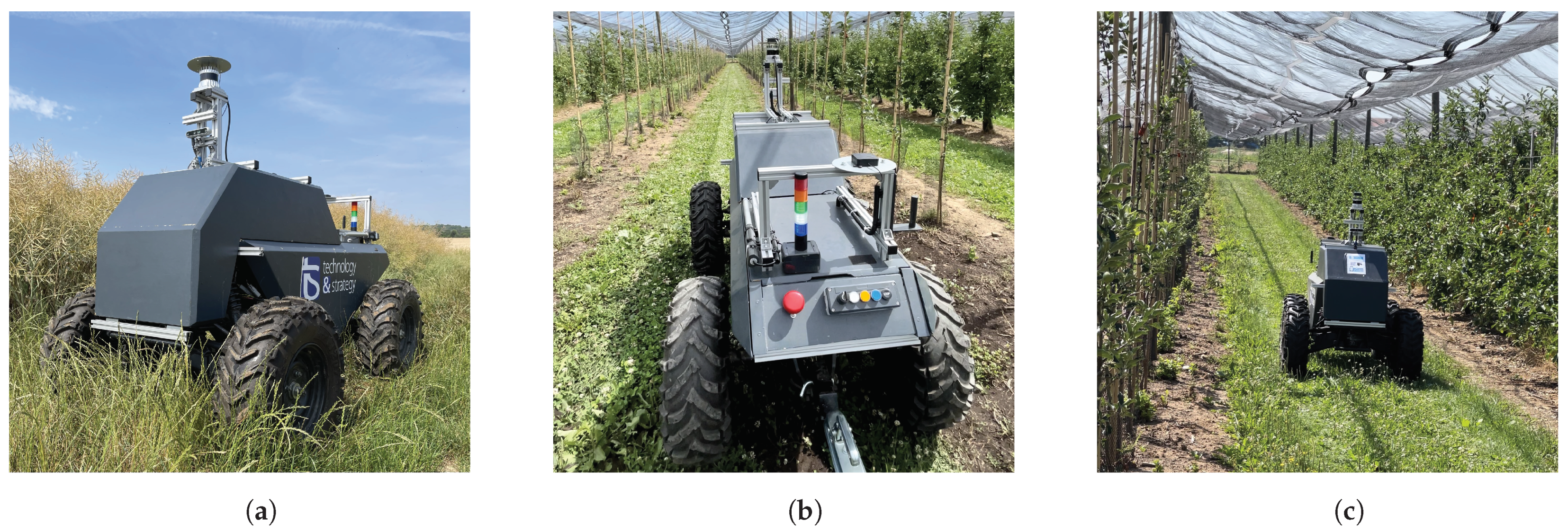
Figure 16.
Pictures of the vehicle prototype on agricultural fields. (a) Front view of the vehicle prototype. (b) Rear view of the robot in an orchard. (c) Front view of the robot in an orchard.
Figure 16.
Pictures of the vehicle prototype on agricultural fields. (a) Front view of the vehicle prototype. (b) Rear view of the robot in an orchard. (c) Front view of the robot in an orchard.
Table 1.
Variables of the 7-DOF model.
Table 1.
Variables of the 7-DOF model.
| Symbol | Description |
|---|
| steering angle |
| associated lateral slip angle of the ith wheel |
| l | wheelbase |
| L | track width |
| longitudinal tire force of the ith wheel |
| lateral tire force of the ith wheel |
Table 2.
Parameter values that were fixed for the weighting functions and for each controller.
Table 2.
Parameter values that were fixed for the weighting functions and for each controller.
| km/h | km/h |
|---|
| | | |
| | | |
| rad/s | rad/s | rad/s | rad/s |
| | | |
| | | |
Table 3.
synthesis performance index.
Table 3.
synthesis performance index.
| |
|---|
| |
Table 4.
Lateral RMS error in trajectory tracking for different longitudinal speeds on rigid soil.
Table 4.
Lateral RMS error in trajectory tracking for different longitudinal speeds on rigid soil.
| | km/h | km/h | km/h |
|---|
| RMS | 0.1231 m | 0.1472 m | 0.1666 m |
Table 5.
Lateral RMS error in trajectory tracking for different longitudinal speeds on sandy soil.
Table 5.
Lateral RMS error in trajectory tracking for different longitudinal speeds on sandy soil.
| | km/h | km/h | km/h |
|---|
| RMS | 0.1235 m | 0.1536 m | 0.1775 m |
Table 6.
Lateral RMS error in trajectory tracking for different tire pressures and longitudinal speeds in real time.
Table 6.
Lateral RMS error in trajectory tracking for different tire pressures and longitudinal speeds in real time.
| | km/h | km/h | km/h |
|---|
| psi = 0.5 bar | 0.0768 m | 0.0743 m | 0.0974 m |
| psi = 0.2 bar | 0.0763 m | 0.0711 m | 0.0703 m |
| Disclaimer/Publisher’s Note: The statements, opinions and data contained in all publications are solely those of the individual author(s) and contributor(s) and not of MDPI and/or the editor(s). MDPI and/or the editor(s) disclaim responsibility for any injury to people or property resulting from any ideas, methods, instructions or products referred to in the content. |
© 2023 by the authors. Licensee MDPI, Basel, Switzerland. This article is an open access article distributed under the terms and conditions of the Creative Commons Attribution (CC BY) license (https://creativecommons.org/licenses/by/4.0/).


