Hybrid Hunter–Prey Optimization with Deep Learning-Based Fintech for Predicting Financial Crises in the Economy and Society

Abstract

Financial technology (Fintech) plays a pivotal role in driving contemporary technology, society, economies, and many other fields. The new-generation Fintech is Smart Fintech, mainly empowered and inspired by data science and artificial intelligence (DSAI) technologies. Smart Fintech combines DSAI and transforms finance and economies for driving automated, intelligent, personalized financial and economic businesses, services and systems, and the whole of business. The strength and growth of the country’s economy were evaluated with the accurate prediction of how many companies will succeed and how many will fail. Financial crisis prediction (FCP) has a considerable effect on the economy. Prior research focuses mainly on deep learning (DL), machine learning (ML), and statistical approaches for forecasting the financial health of a company. Thus, this study presents a hybrid hunter–prey optimization with a deep learning-based FCP (HHPODL-FCP) technique. The objective of the HHPODL-FCP algorithm lies in the effective identification of the financial crisis in enterprises or organizations. To accomplish this, the HHPODL-FCP method makes use of the HHPO algorithm for the feature subset selection process. In addition, the HHPODL-FCP technique employs the gated attention recurrent network (GARN) model for the identification and classification of financial and non-financial crises. The HHPODL-FCP method exploits a sparrow search algorithm (SSA)-based hyperparameter tuning process to enrich the performance of the GARN model. The simulation results of the HHPODL-FCP method are tested on different financial datasets. A wide range of experiments highlighted the remarkable performance of the HHPODL-FCP method over recent techniques under various measures.

1. Introduction

Financial crisis prediction (FCP) is rooted in the recognition of the significant economic and social impacts that financial crises can have on a global scale. Financial crises can result in huge economic losses, unemployment, and losses in asset values, leading to considerably affected businesses and individuals. Almost two-thirds of chief economists believe a global recession is likely in 2023, of which 18% consider it extremely likely—more than twice as many as in the previous survey conducted in September 2022 [1]. Lately, finance has become increasingly interactive with next-generation data science and artificial intelligence (DSAI) technologies. In particular, Fintech is at the epicenter of synthesizing, innovating, and transforming communication technologies, economy, society, media, and financial services largely driven by DSAI technologies [1]. With advances in the financial crisis of businesses worldwide, the financial organization has gained popularity in the field of FCP in recent years [2]. There is a need to develop reliable and earlier predictive techniques for enterprises or financial companies to forecast the potential risks of the business status [3].

FCP helps financial institutions in making decisions at the proper time for sustainable growth. Usually, FCP yields a binary classification algorithm that is rationally resolved. Incorrect decision-making in a corporation might lead to economic failure or bankruptcy and affects investors, clients, vendors, etc. The ongoing development in the field of information technology enables accomplishing all kinds of data closely related to the risk levels of enterprises. A large number of people depend on the predictor decision to assess a wide range of information [4]. But, various factors may have a direct impact on performance assessment. Statistical and AI technologies are used for the detection of FCP. AI can be used in different ways in FCP, which builds a model that predicts whether the financial organization may suffer a crisis or not [5]. Using economic and other financial details from the tactical competitiveness of the organization to develop an efficient method can be challenging [6]. Except for AI and databases, data mining technology is more commonly utilized in other methods. Early warning and decision-making are two different strategies of FCP exploited in data mining [7]. Then, it assists financial decision-makers to select and evaluate the business for investment or collaboration. In-depth analysis of data needs less computational time and more resources. It is difficult to filter data with erroneous information [8]. Therefore, the process of extracting a vast amount of data plays an important role in identifying financial failure, particularly for FCP [9]. In data mining, feature selection (FS) is a pre-processing step. Also, it filters the redundant and repetitive features from the original information. Prior research focuses on deep learning (DL), machine learning (ML), and statistical algorithms for forecasting the financial status of a business [10]. Model training with hyperparameters finetuning has become one of the main constraints.

This study proposes a hybrid hunter–prey optimization with the deep learning-based FCP (HHPODL-FCP) technique. The HHPODL-FCP technique makes use of the HHPO algorithm for the feature subset selection process. In addition, the HHPODL-FCP technique employs the gated attention recurrent network (GARN) model for the identification and classification of financial and non-financial crises. The HHPODL-FCP technique exploits a sparrow search algorithm (SSA)-based hyperparameter tuning process to enrich the performance of the GARN model. The simulation results of the HHPODL-FCP technique are tested on different financial datasets.

2. Related Works

Tyagi and Boyang [11] present a smart IoT-enabled FCP using a metaheuristic algorithm. Initially, the enterprise data are aggregated by IoT gadgets, namely laptops, smartphones, etc. In the next stage, the quantum artificial butterfly optimization (QABO) technique for FS is used to optimize the selection of feature subsets. Then, LSTM with RNN is applied for the classification of collected financial information. Muthukumaran and Hariharanath [12] consider the design of the optimum DL-based FCP (ODL-FCP) method for SMEs. The presented method integrates two stages: optimal deep CNN with LSTM (DCNN-LSTM)-based data classification and Archimedes optimization algorithm-based FS (AOA-FS) procedure.

Muthukumaran et al. [13] propose a new multi- vs. optimization (MVO)-based FS with an optimum variational autoencoder (OVAE) system for the FCP. The MVO technique-based FS with the OVAE (MVOFS-OVAE) system mainly achieves forecasting of economic failure. To achieve this, the presented method mainly pre-processes the data with the help of min–max normalization. Furthermore, the presented technique develops a feature subset selection process. Then, the VAE mode is used for the classification of economic information into non-financial or financial crises. Lastly, for the hyperparameter tuning of the VAE, the study used the differential evolution (DE) technique. Mohan et al. [14] introduce an eagle strategy arithmetical optimization algorithm with optimum deep convolutional forest (ESAOA-ODCF)-based Fintech applications for hyper-automation.

Bhattacharya et al. [15] devised an MGWO-SAE (modified grey wolf optimizer with SAE) for FCP scenarios in smaller marginal firms. To achieve this, the presented algorithm applies data pre-processing to convert the input dataset into an accurate form. This study adopts the SAE classification technique for prediction. Al Duhayyim et al. [16] introduce a new multiobjective squirrel search optimization approach with SAE (MOSSA-SAE) for the FCP in the IoT platform. At first, this technique enables IoT devices, namely laptops, smartphones, and so on, to collect the financial data of users that are later transferred onto the cloud for more detailed investigation. Furthermore, the SMOTE method is used to deal with class imbalance problems. The objective is to define the over-sampling rate and region of nearby neighbors of SMOTE. In addition, the SAE system is used as a classification model for determining the class labels of financial details.

An OALOFS-MLC (oppositional ant lion optimizer-based FS with ML-assisted classification) algorithm for the FCP was developed by Venkateswarlu et al. [17]. The Hadoop MapReduce tool is applied for big data management. Additionally, a new OALOFS technique was introduced for selecting an optimum set of features that assist in achieving high efficiency of classification. Also, the DRVFLN (deep random vector functional link network) architecture is exploited to carry out the grading process. With the integration of improved grey wolf optimization (IGWO) and a fuzzy neural classifier (FNC), Sankhwar et al. [18] proposed a new predictive model for the FCP. The proposed model is derived by integrating the tumbling effect and GWO algorithm. The proposed technique is used to find the optimum features from the financial details.

Most of the existing models do not focus on the hyperparameter selection process, which mainly influences the performance of the classification model. Particularly, hyperparameters such as epoch count, batch size, and learning rate selection are essential to attain effectual outcomes. Since the trial and error method for hyperparameter tuning is a tedious and erroneous process, metaheuristic algorithms can be applied. Therefore, in this work, we employ the SSA algorithm for parameter selection of the GARN model.

3. The Proposed Model

In this study, we focused on the development of the HHPODL-FCP technique for the Fintech environment. The purpose of the HHPODL-FCP method lies in the effective identification of the economic crisis in a firm or organization. To accomplish this, the HHPODL-FCP algorithm exploits three distinct processes, namely SSA-based hyperparameter tuning, GARN-based prediction, and HHPO-based FS. Figure 1 displays the overall procedure of the HHPODL-FCP methodology.

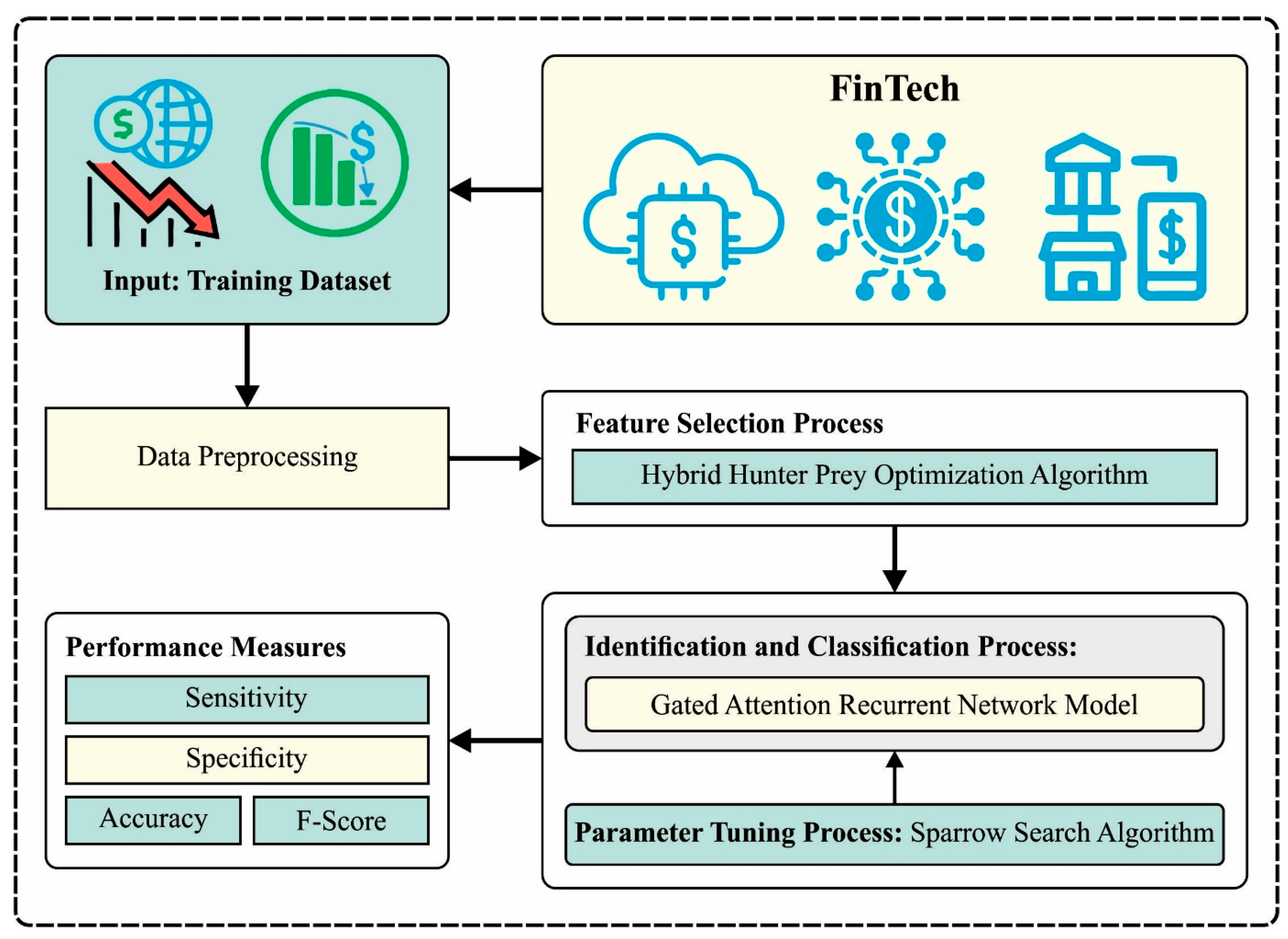
3.1. Design of HHPO-Based Feature Selection

At the primary stage, the HHPO algorithm is used to choose an optimal set of features [19]. In the HPO technique, the search process for the hunter is expressed by Equation (1).

$$x_{i,j}\left(t+1\right)=x_{i,j}\left(t\right)+0.5\left[2cZ{P}_{pos\left(j\right)}-x_{i,j}\left(t\right)\right]+\left(2\left(1-c\right)Zm\left(j\right)-x_{i,j}\left(t\right)\right)$$

(1)

The variable $x_{i,j}\left(t\right)$ defines the predator’s location, and $P_{pos}$ stands for the place of prey. Additionally, $m\left(j\right)$ represents the mean of every position, and $Z$ denotes the adaptive parameter calculated by employing Equation (2).

$$\begin{gathered} P={\overrightarrow{R}}_1<c;IDX=\left(P==0\right); \\ Z=R_2\otimes IDX+{\overrightarrow{R}}_3\otimes \left(\sim IDX\right) \end{gathered}$$

(2)

where ${\overrightarrow{R}}_1$ and ${\overrightarrow{R}}_3$ imply the stochastic vector in the range of zero and one$,$ $R_2$ defines the randomly generated number in the interval [$0,1$], and $IDX$ suggests the index amount of the vector which fulfills the $\left(P==0\right)$ condition.

The key parameter $c$ is used to balance among exploration and exploitation stages whose value slowly reduces from a primary value of $1$ to a minimal threshold of 0.02. This value can be defined by applying Equation (3).

$$c=1-T\left(\frac{0.98}{T_{\mathrm{m}\mathrm{a}\mathrm{x}}}\right)$$

(3)

Afterward, the purpose of the prey position $P_{pos}$ proceeds by primary computation of the mean $m$ of every position expressed by Equation (4), then, the distance calculation $D_{euc}$ among the entire individual is studied, and the mean position is written in Equation (5).

$$m=\frac{1}{n}\sum _{i=1}^n{x}_i$$

(4)

$$D_{euc\left(i\right)}={\left(\sum _{j=1}^d{\left(x_{i,j}-m_j\right)}^2\right)}^{\frac{1}{2}}$$

(5)

If you engage in hunting performances, it is general practice to hunt for capturing and chasing prey, which leads to the death of the prey. Then, the hunters need to find a novel place to endure hunting. To overcome the convergence issue, which is inherent in the present method as demonstrated in Equation (6), it can be suggested to execute a diminishing process.

$$k=round\left(c\times N\right)$$

(6)

where $\mathrm{t}\mathrm{h}\mathrm{e}N$ parameter implies the count of searching populations from the optimizer manner. In the beginning, the $k$ value corresponded to the size of the population. The farthermost searching individuals in the selected target $m$ are labeled as prey $P_{pos}$ and are consequently caught by the hunters. For determining the prey’s place $P_{pos},$ Equation (7) is established in Equations (4)–(6) over a rigorous analytical procedure.

$$P_{pos}=x_i|iissorted{D}_{euc}\left(k\right)$$

(7)

If the prey anticipates the attack, it will instinctively search for refuge in a safe place. It can be assumed that the optimum safe place is none except the global optimum location, as it gives the prey the highest possibility of survival. Subsequently, the predator drive chooses a novel prey location, which can be obtained by employing Equation (8) for updating the prey’s location.

$$x_{i,j}\left(t+1\right)=T_{pos\left(j\right)}+cZ \mathrm{c}\mathrm{o}\mathrm{s}\left(2\pi R_4\right)\times \left[T_{pos\left(j\right)}-x_{i,j}\left(t\right)\right]$$

(8)

where the present prey places are defined by the parameter $x_{i,j}\left(t\right)$, which is a critical element in the optimizer method. The global optimal location is represented by $T_{pos\left(j\right)}$, but the variable $R_4$ refers to the arbitrary number in the range [0, 1]. The $\mathrm{c}\mathrm{o}\mathrm{s}$ function and the input parameters can be employed for calculating the next location of prey that is tactically located at a distinct radius and angle in the global optimal location for enhancing the method. The purpose of the prey and hunter is accomplished by configuring the alteration $\beta$ parameter that is presented at a value of $0.1$. Additionally, the parameter $R_5$ is an arbitrarily created number within [$\mathrm{0,1}$]. Particularly, the hunter location can be updated by Equation (1) if $R_5<\beta$, while Equation (8) is used for updating the prey location.

In the design of the HHPO algorithm, the Tent chaos mapping and opposition-based learning (OBL) approach called TOBL was proposed to enhance population quality. The population intelligence optimization algorithm widely uses random generation for initializing the population. This nonuniform distribution has a direct impact on the convergence rate and performance of the optimization technique for identifying the optimum result. Good traversal, chaotic sequence, and possessing diversity characteristics were introduced as promising solutions to these issues. Prey population, which integrates chaotic sequences, namely cubic mapping, Tent mapping, logistic mapping, and circle mapping, exhibits the best diversity Tent chaotic mapping, described by better convergence speed and traversal uniformity, which creates a uniform distribution chaotic sequence in the interval of $[0,1]$.

The formula of Tent chaotic mapping is shown as follows:

$$y_{t+1}=\left\{\begin{array}{ll}{y}_t/a& 0\le y_t<a\\ \left(1-y_t\right)/(1-a)& a\le y_t\le 1\end{array}\right.$$

(9)

In Equation (9), $y_t$ indicates the amount of chaos produced after $T$ iterations, $T=\mathrm{0,1},$ $\cdots ,$ $T_{\mathrm{m}\mathrm{a}\mathrm{x}}$, whereas $a$ shows a constant between $\left[0,1\right].$ By using a uniform variation of Tent, the TOBL approach includes dynamic compression of the distribution range with the sum of lower and upper boundaries of the objective function. The final objective is to guarantee uniformity in the population.

$${\overline{x}}_{i,j}=l{b}_j+u{b}_j-y_i\otimes x_{i,j}$$

(10)

The steps of the TOBL algorithm are given in the following: consider an $n$ number of populations. First, $\mathrm{t}\mathrm{h}\mathrm{e}n$ population position was generated at random, then, the $n$ chaotic opposing position was generated by TOBL, and then, $\mathrm{t}\mathrm{h}\mathrm{e}2n$ position was ranked with respect to fitness, and the top $n$ position was chosen as the initial population.

The TOBL approach includes the following subsequent stages: assume a population size of $n$; initially, the $n$ population position was randomly generated. Next, the $n$ chaotic opposing position was produced by the TOBL. Later, based on the respective fitness level, the $2n$ position was ranked, and the top $n$ position was chosen for the population initialization.

In the HHPO approach, FF is used to balance the classification accuracy (maximal) and the number of features selected in the solution (minimal). Equation (11) represents the FF to estimate the solution.

$$Fitness=\alpha {\gamma }_R\left(D\right)+\beta \frac{\left|R\right|}{\left|C\right|}$$

(11)

where $\left|R\right|$ denotes the cardinality of the selected subset, ${\gamma }_R\left(D\right)$ shows the classification error rate of a given classifier. $\left|C\right|$ refers to the overall amount of features in the dataset, and the two parameters $\alpha$ and $\beta$ correspond to the significance of classification quality and subset length. ∈ [1, 0] and $\beta =1-\alpha .$

3.2. FCP Using GARN Model

For the identification and classification of financial and non-financial crises, the GARN model is used. GARN is a hybrid model of BiGRU with the attention model [20]. Due to the application of recurrent neural networks (RNN), numerous challenges take place since it exploits old data instead of the existing data for classification. A bidirectional RNN (BRNN) is used to resolve these problems that utilize existing and old data. Hence, two RNNs are employed to implement the forward and reverse functions.

The output was interconnected to the output layer for recording the feature sequence. An additional bidirectional gated recurrent unit (BiGRU) was proposed based on the BRNN model, where the hidden layer (HL) of BRNN was replaced with one GRU memory module. Now, the gated attention recurrent network (GARN) is a combination of BiGRU with the attention module, and its architecture is shown in Figure 2.

Assume an $m$-dimension input dataset as $(y_1,y_2,\dots .,y_m)$. HL in the BGRU generates an output $H_{t_1}$ at the $t_{het1}$ time given below:

$$\overrightarrow{H}=\sigma \left(w_{e_{\overrightarrow{yH}}}{y}_{t_1}+w_{e_{\overrightarrow{H}\overrightarrow{H}}}{\overrightarrow{H}}_{t_1-1}+c_{\overrightarrow{H}}\right)$$

(12)

$${\overleftarrow{H}}_{t_1}=\sigma \left(w_{e_{\overleftarrow{yH}}}{y}_{t_1}+w_{e_{\overleftarrow{H}\overleftarrow{H}}}{\overleftarrow{H}}_{t_1-1}+c_{\overleftarrow{H}}\right)$$

(13)

$$H_{t_1}={{\overrightarrow{H}}_t}_1\oplus {\overleftarrow{H}}_{t_1}$$

(14)

From the expression, ${{\overrightarrow{H}}_t}_1$ and ${\overleftarrow{H}}_{t_1}$represent the positive and negative outputs of GRU. The weighting factor for two connected layers is represented by $w_e,$ $\oplus$ denotes the bitwise operator, $c$ shows the bias vector, and $\sigma$ indicates the activation function.

3.3. Hyperparameter Tuning Using SSA

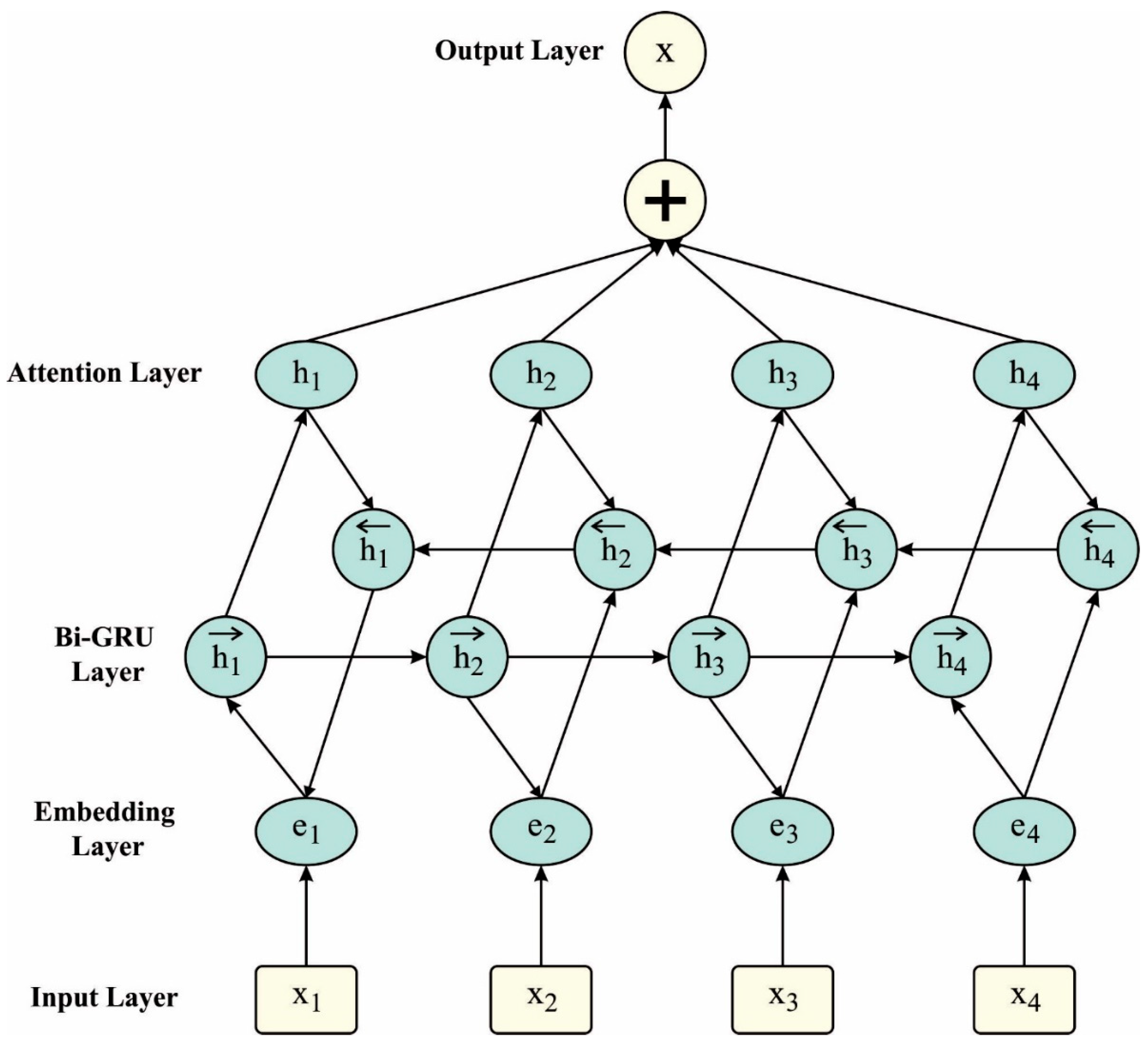
The SSA is applied in this study to adjust the hyperparameter values of the GARN model. SSA is a metaheuristic optimization technique based on the foraging and anti-predation behaviors of sparrows [21]. In this work, discoverers, followers, and watchers are three different strategies of individuals in SSA. The mathematical expression and natural behaviors of sparrows were defined as follows:

Discoverers: All the generations of discoverers signify a point in the population, i.e., nearer to food, and their major objective is to provide direction for the whole population to search for food. The formula for the updating position of the discoverers can be given as the following:

$$x_{i,j}^{t+1}=\left\{\begin{array}{l}{x}_{i,j}^t\cdot \mathrm{e}\mathrm{x}\mathrm{p}\left(\frac{-i}{\alpha \times iie{r}_{\mathrm{m}\mathrm{a}\mathrm{x}}}\right),R_2<ST\\ x_{i,j}^t+Q\cdot L,\hspace{1em}\hspace{1em}{R}_2\ge ST\end{array}\right.$$

(15)

In Equation (15),$ite{r}_{\mathrm{m}\mathrm{a}\mathrm{x}}$ shows the maximal amount of iterations, $x_{i,j}^t$ denotes the location of the $i^{th}$ sparrows in the $j^{th}$ dimension at$t$ iterations, $ST$ indicates the safety threshold, $R_2$ and $\alpha$ represents randomly generated values within [$0,1$], $L$ stands for the vector with the element, and$Q$ denotes the uniformly distributed random integer. If $R_2<ST,$ the discoverers can extensively search for food. If $R_2\ge ST$ then there is danger, and the discoverers must withdraw from the danger zone.

Followers: The follower’s role is to follow the discoverers searching for food. The updating strategy can be given below:

$$x_{i,j}^{t+1}=\left\{\begin{array}{l}Q\cdot \mathrm{e}\mathrm{x}\mathrm{p}\left(\frac{x_{worst}^t-x_{i,i}^t}{i^2}\right),ifi>n/2\\ x_{best}^{t+1}+\left|x_{i,j}-x_{best}^{t+1}\right|\cdot A^{+}\cdot L,otherwise\end{array}\right.$$

(16)

In Equation (16), $\mathrm{I}>n/2$ shows that the present follower is in a poor location and extensively searches for food by deviating from the worst individuals; or else, the food search can be done by competing with other optimal individuals.$A$ indicates the random vector with values of $1$ or $-1$ for all the elements, ${x_{best}^{t+1}\mathrm{a}\mathrm{n}\mathrm{d}x}_{worst}^t$, correspondingly showing the individuals with the best individuals and worst current fitness.

Vigilantes are random proportions of an individual in the population whose primary task is to alert the foraging region. The formula can be given as follows:

$$x_{i,j}^{t+1}=\left\{\begin{array}{ll}{x}_{best}^t+\beta \cdot \left|x_{i,j}^t-x_{best}^t\right|,& f_i\ne f_g\\ x_{best}+k\cdot \left(\frac{x_{i,i}^t-x_{best}^t}{\left|f_i-f_w\right|+\epsilon }\right),& f_i=f_g\end{array}\right.$$

(17)

In Equation (17), $k$ shows the random value between $-1$ and $1$; $f_i,$ $f_g$, and $f_w$ represent the fitness function of the existing alert, optimum, and worst individuals, correspondingly; $\beta$ denotes the update step with a mean of $0$ and variance of $1$; and $\epsilon$ is used to prevent a constant with a denominator of $0.$ The sparrow individual at the center of the population feels threatened if $f_i=f_g$, and move towards its species, which reduces the predation risk; and the sparrow at the edge of the population if $f_i\ne f_g$ and thereby approaches other optimum individuals.

The SSA approach derives a fitness function from obtaining the high efficiency of the GARN classification model. The fitness function describes a positive integer to represent the best outcomes of the solution candidate. The decline in the classification error rate can be defined as a FF.

$$\begin{gathered} fitness\left(x_i\right)=ClassifierErrorRate\left(x_i\right) \\ \hspace{1em}\hspace{1em}\hspace{1em}\hspace{1em}\hspace{1em}=\frac{numberofmisclassifiedsamples}{Totalnumberofsamples}*100 \end{gathered}$$

(18)

4. Results and Discussion

The proposed model is simulated using the Python 3.6.5 tool on PC i5-8600k, GeForce 1050Ti 4 GB, 16 GB RAM, 250 GB SSD, and 1 TB HDD. The parameter settings are given as follows: learning rate: 0.01, dropout: 0.5, batch size: 5, epoch count: 50, and activation: ReLU. In this work, the FCP outcomes of the HHPODL-FCP technique are examined on two datasets such as German credit [22] and Australian credit [23].

Table 1. Details of two datasets.

Dataset	No. of Instances	No. of Attributes	No. of Class	Financial Crisis/Non-Financial Crisis
German Credit	1000	24	2	300/700
Australian Credit	690	14	2	383/307

defines the details of the two datasets.

The FS results of the HHPO algorithm are shown in

Table 2. Details of selected features.

Dataset	Selected Features
German Credit	2, 4, 6, 8, 9, 11, 13, 14, 15, 16, 18, 21, 23
Australian Credit	1, 3, 6, 8, 10, 12, 13

. The table values indicate the features chosen by the HHPO algorithm on two datasets.

The best cost (BC) results of the HHPODL-FCP method with other FS techniques are reported in

Table 3. BC analysis of the HHPODL-FCP method with other FS methods on two datasets.

No. of Iterations	German Credit Dataset
	HHPODL-FCP	QABO-FS	ACO-FS	GWO-FS
1	0.116	0.143	0.150	0.170
2	0.116	0.143	0.150	0.170
3	0.116	0.143	0.150	0.150
4	0.116	0.143	0.150	0.150
5	0.122	0.143	0.140	0.150
6	0.122	0.143	0.140	0.150
7	0.122	0.143	0.140	0.150
8	0.102	0.122	0.140	0.150
9	0.102	0.122	0.130	0.150
10	0.099	0.114	0.130	0.150
Average	0.114	0.136	0.142	0.154
No. of Iterations	Australian Credit Dataset
	HHPODL-FCP	QABO-FS	ACO-FS	GWO-FS
1	0.043	0.054	0.074	0.089
2	0.043	0.054	0.073	0.089
3	0.043	0.054	0.073	0.089
4	0.043	0.054	0.073	0.089
5	0.036	0.043	0.073	0.087
6	0.036	0.043	0.073	0.085
7	0.032	0.042	0.073	0.085
8	0.032	0.042	0.073	0.085
9	0.032	0.042	0.073	0.085
10	0.031	0.041	0.073	0.085
Average	0.037	0.047	0.073	0.087

and Figure 3. The outcomes demonstrate that the HHPODL-FCP technique offers superior results with optimal BC values on both datasets. For instance, on the German Credit dataset, the HHPODL-FCP technique provides a BC of 0.114 while the QABO-FS, ACO-FS, and GWO-FS systems offer an increasing BC of 0.136, 0.142, and 0.154, correspondingly. Finally, on the Australian Credit dataset, the HHPODL-FCP algorithm offers a BC of 0.037 while the QABO-FS, ACO-FS, and GWO-FS approaches are given to improve BC of 0.047, 0.073, and 0.087, correspondingly.

Figure 4 demonstrates the training accuracy $TR\_acc{u}_y$ and $VL\_acc{u}_y$ of the HHPODL-FCP method on the German Credit dataset. The $TL\_acc{u}_y$ is resolved by analyzing the HHPODL-FCP approach on the TR dataset, while the $VL\_acc{u}_y$ is computed by estimating the performance on an individual testing dataset. The outcomes reveal that $TR\_acc{u}_y$ and $VL\_acc{u}_y$ improve with an upsurge in epochs. Hence, the performance of the HHPODL-FCP model was enhanced on the TR and TS datasets with an increase in the number of epochs.

In Figure 5, the $TR\_loss$ and $VR\_loss$ analysis of the HHPODL-FCP algorithm on the German Credit dataset is shown. The $TR\_loss$ determines the error between the prediction performance and original values on the TR data. The $VR\_loss$ denoted the evaluating performance of the HHPODL-FCP system on validation data. The outcomes signify that the $TR\_loss$ and $VR\_loss$ tend to reduce with increasing epochs. It represents the better performance of the HHPODL-FCP model and its proficiency in generating accurate classification. The diminished value of $TR\_loss$ and $VR\_loss$ exhibits the higher performance of the HHPODL-FCP method in capturing relationships and patterns.

Figure 6 shows the training accuracy $TR\_acc{u}_y$ and $VL\_acc{u}_y$ of the HHPODL-FCP approach on the Australian Credit dataset. The $TL\_acc{u}_y$ is defined by the estimation of the HHPODL-FCP model on the TR dataset when the $VL\_acc{u}_y$ is computed by measuring the performance on a different testing dataset. The results reveal that $TR\_acc{u}_y$ and $VL\_acc{u}_y$ enhanced with an upsurge in epochs. As a consequence, the performance of the HHPODL-FCP algorithm reached better on the TR and TS dataset with an increase in the number of epochs.

In Figure 7, the $TR\_loss$ and $VR\_loss$ outcomes of the HHPODL-FCP system on the Australian Credit dataset are illustrated. The $TR\_loss$ describes the error between the prediction performance and original values on the TR data. The $VR\_loss$ signifies measuring the performance of the HHPODL-FCP model on separate validation data. The outcomes denote that the $TR\_loss$ and $VR\_loss$ tend to reduce with increasing epochs. It represents the improved performance of the HHPODL-FCP model and its ability to generate accurate classification. The decreased value of $TR\_loss$ and $VR\_loss$ exhibits the greater performance of the HHPODL-FCP technique in capturing patterns and relationships.

The comparative FCP outcomes of the HHPODL-FCP technique on the German Credit dataset are depicted in

Table 4. Comparative outcome of the HHPODL-FCP method with other techniques on the German Credit dataset.

German Credit Dataset
Classifiers	$\mathit{S}\mathit{e}\mathit{n}{\mathit{s}}_{\mathit{y}}$	$\mathit{S}\mathit{p}\mathit{e}{\mathit{c}}_{\mathit{y}}$	$\mathit{A}\mathit{c}\mathit{c}{\mathit{u}}_{\mathit{y}}$	${\mathit{F}}_{\mathit{s}\mathit{c}\mathit{o}\mathit{r}\mathit{e}}$
HHPODL-FCP	93.51	93.97	94.87	93.67
QABO-LSTM-RNN	87.18	93.53	91.91	90.06
LSTM-RNN	82.14	88.5	84.53	88.69
ACO Model	78.27	69.25	75.72	85.35
MLP Algorithm	73.81	66.83	70.9	75.07
SVM Model	72.64	66.37	71.12	71.71
AdaBoost	71.34	61.28	67.48	71.22

and Figure 8 [11]. The outcomes notified that the LSTM-RNN, ACO, MLP, SVM, and AdaBoost methods had shown poor FCP results over other models. Additionally, the QABO-LSTM-RNN method obtained moderate FCP performance with $sen{s}_y$, $spe{c}_y$, $acc{u}_y$, and $F_{score}$ of 87.18%, 93.53%, 91.91%, and 90.06%, respectively. Nevertheless, the HHPODL-FCP technique reports promising results with maximum $sen{s}_y$, $spe{c}_y$, $acc{u}_y$, and $F_{score}$ of 93.51%, 93.97%, 94.87%, and 93.67%, correspondingly.

A comparison of FCP analysis of the HHPODL-FCP approach on the Australian Credit dataset is shown in

Table 5. Comparative outcome of the HHPODL-FCP technique with other methods on the Australian Credit dataset.

Australian Credit Dataset
Classifiers	$\mathit{S}\mathit{e}\mathit{n}{\mathit{s}}_{\mathit{y}}$	$\mathit{S}\mathit{p}\mathit{e}{\mathit{c}}_{\mathit{y}}$	$\mathit{A}\mathit{c}\mathit{c}{\mathit{u}}_{\mathit{y}}$	${\mathit{F}}_{\mathit{s}\mathit{c}\mathit{o}\mathit{r}\mathit{e}}$
HHPODL-FCP	94.31	94.55	95.04	94.63
QABO-LSTM-RNN	90.90	93.16	93.31	94.64
LSTM-RNN	85.97	93.02	93.02	91.61
ACO Model	79.73	89.31	89.65	81.91
MLP Algorithm	76.48	84.41	84.39	78.68
SVM Model	71.09	75.66	76.11	77.38
AdaBoost	69.07	67.30	67.65	68.43

and Figure 9. The outcomes reported that the LSTM-RNN, ACO, MLP, SVM, and AdaBoost systems have revealed poor FCP results over other methods.

The QABO-LSTM-RNN technique has managed to acquire modest FCP performance with $sen{s}_y$, $spe{c}_y$, $acc{u}_y$, and $F_{score}$ of 90.90%, 93.16%, 93.31%, and 94.64%, correspondingly. However, the HHPODL-FCP method reported positive results with the highest $sen{s}_y$, $spe{c}_y$, $acc{u}_y$, and $F_{score}$ of 94.31%. 94.55%, 95.04%, and 94.63%, correspondingly.

The computation time (CT) analysis of the HHPODL-FCP technique on two datasets is reported in

Table 6. CT outcome of the HHPODL-FCP approach with other techniques on two datasets.

Computational Time (sec)
Classifiers	German Credit Dataset	Australian Credit Dataset
HHPODL-FCP	0.23	0.40
QABO-LSTM-RNN	1.23	1.40
LSTM-RNN	2.27	3.35
ACO Model	1.30	1.37
MLP Algorithm	3.22	2.37
SVM Model	1.28	4.33
AdaBoost	2.28	3.47

. The outcomes ensured that the HHPODL-FCP technique required the least CT values on both datasets. For instance, on the German Credit dataset, the HHPODL-FCP technique provided a minimal CT of 0.23 s while the QABO-LSTM-RNN, LSTM-RNN, ACO, MLP, SVM, and AdaBoost models offered a maximum CT of 1.23 s, 2.27 s, 1.30 s, 3.22 s, 1.28 s, and 2.28 s, respectively. Finally, on the Australian Credit dataset, the HHPODL-FCP model offered a minimum CT of 0.40 s, whereas the QABO-LSTM-RNN, LSTM-RNN, ACO, MLP, SVM, and AdaBoost technique obtained the highest CT of 1.40 s, 3.35 s, 1.37 s, 2.37 s, 4.33 s, and 3.47 s, correspondingly. These results guaranteed the accurate and effectual FCP results of the HHPODL-FCP technique.

5. Conclusions

In this study, we focused on developing the HHPODL-FCP technique for the Fintech environment. The purpose of the HHPODL-FCP method lies in the effective identification of the financial crisis in a firm or organization. To accomplish this, the HHPODL-FCP technique exploits three distinct processes, namely HHPO-based FS, GARN-based prediction, and SSA-based hyperparameter tuning. Moreover, the HHPODL-FCP algorithm employed the GARN model for the identification and classification of financial and non-financial crises. The HHPODL-FCP technique exploited the SSA-based hyperparameter tuning process to enhance the performance of the GARN algorithm. The simulation results of the HHPODL-FCP technique are tested on different financial datasets. A wide range of experiments highlighted the remarkable performance of the HHPODL-FCP technique over recent techniques under various measures. The enhanced performance of the proposed model is due to the inclusion of HHPO-based FS and SSA-based hyperparameter tuning processes. The HHPODL-FCP model provides an effective solution for the identification of significant financial crises, which enables policymakers, financial institutions, and investors to take proactive measures and alleviate the adversative effects of financial crises. Future work could focus on the design of automated DL models for financial fraud. In addition, the proposed model can be tested on large-scale real-time datasets in the future.

References

1. Available online: https://www.weforum.org/press/2023/01/chief-economists-say-global-recession-likely-in-2023-but-cost-of-living-crisis-close-to-peaking/#:~:text=Almost%20two%2Dthirds%20of%20chief,to%20be%20unlikely%20this%20year (accessed on 14 April 2023).
2. Khuwaja, P.; Khowaja, S.A.; Dev, K. Adversarial learning networks for fintech applications using heterogeneous data sources. IEEE Internet Things J. 2021, 10, 2194–2201. [Google Scholar] [CrossRef]
3. Bazarbash, M. Fintech in Financial Inclusion: Machine Learning Applications in Assessing Credit Risk; International Monetary Fund: Washington, DC, USA, 2019. [Google Scholar]
4. Ceron, B.M.; Monge, M. Financial Technologies (FINTECH) Revolution and COVID-19: Time Trends and Persistence. Rev. Dev. Financ. 2023, 13, 58–64. [Google Scholar]
5. Bluwstein, K.; Buckmann, M.; Joseph, A.; Kapadia, S.; Şimşek, Ö. Credit growth, the yield curve and financial crisis prediction: Evidence from a machine learning approach. J. Int. Econ. 2023, 103773. [Google Scholar] [CrossRef]
6. Balmaseda, V.; Coronado, M.; de Cadenas-Santiagoc, G. Predicting Systemic Risk in Financial Systems Using Deep Graph Learning. Intell. Syst. Appl. 2023, 19, 200240. [Google Scholar] [CrossRef]
7. Uthayakumar, J.; Metawa, N.; Shankar, K.; Lakshmanaprabu, S.K. An intelligent hybrid model for financial crisis prediction using machine learning techniques. Inf. Syst. e-Bus. Manag. 2020, 18, 617–645. [Google Scholar] [CrossRef]
8. Liu, L.; Chen, C.; Wang, B. Predicting financial crises with machine learning methods. J. Forecast. 2022, 41, 871–910. [Google Scholar] [CrossRef]
9. Dominic, D.P.; Adimoolam, M.; Balamurugan, N.M. Share Market Data Prediction Strategies Using Deep Learning Algorithm. Recent Adv. Comput. Sci. Commun. 2019. [Google Scholar] [CrossRef]
10. Kočišová, K.; Mišanková, M. Discriminant analysis as a tool for forecasting company’s financial health. Procedia-Soc. Behav. Sci. 2014, 110, 1148–1157. [Google Scholar] [CrossRef] [Green Version]
11. Tyagi, S.K.S.; Boyang, Q. An intelligent internet of things aided financial crisis prediction model in fintech. IEEE Internet Things J. 2021, 10, 2183–2193. [Google Scholar] [CrossRef]
12. Muthukumaran, K.; Hariharanath, K. Deep Learning Enabled Financial Crisis Prediction Model for Small-Medium Sized Industries. Intell. Autom. Soft Comput. 2022, 35, 521–536. [Google Scholar] [CrossRef]
13. Muthukumaran, K.; Hariharanath, K.; Haridasan, V. Feature Selection with Optimal Variational Auto Encoder for Financial Crisis Prediction. Comput. Syst. Sci. Eng. 2023, 45, 887–901. [Google Scholar] [CrossRef]
14. Mohan, P.; Neelakandan, S.; Mardani, A.; Maurya, S.; Arulkumar, N.; Thangaraj, K. Eagle Strategy Arithmetic Optimisation Algorithm with Optimal Deep Convolutional Forest Based FinTech Application for Hyper-automation. Enterp. Inf. Syst. 2023, 2188123. [Google Scholar] [CrossRef]
15. Bhattacharya, R.; Krishna, S.H.; Haralayya, B.; Nagpal, P. Modified Grey Wolf Optimizer with Sparse Autoencoder for Financial Crisis Prediction in Small Marginal Firms. In Proceedings of the 2023 Second International Conference on Electronics and Renewable Systems (ICEARS), Tuticorin, India, 2–4 March 2023; pp. 907–913. [Google Scholar]
16. Al Duhayyim, M.; Alsolai, H.; Al-Wesabi, F.N.; Nemri, N.; Mahgoub, H.; Hilal, A.M.; Hamza, M.A.; Rizwanullah, M. Optimized stacked autoencoder for IoT enabled financial crisis prediction model. CMC-Comput. Mater. Contin. 2022, 71, 1079–1094. [Google Scholar]
17. Venkateswarlu, Y.; Baskar, K.; Wongchai, A.; Gauri Shankar, V.; Paolo Martel Carranza, C.; Gonzáles, J.L.A.; Murali Dharan, A.R. An efficient outlier detection with deep learning-based financial crisis prediction model in big data environment. Comput. Intell. Neurosci. 2022, 2022, 4948947. [Google Scholar] [CrossRef] [PubMed]
18. Sankhwar, S.; Gupta, D.; Ramya, K.C.; Sheeba Rani, S.; Shankar, K.; Lakshmanaprabu, S.K. Improved grey wolf optimization-based feature subset selection with fuzzy neural classifier for financial crisis prediction. Soft Comput. 2020, 24, 101–110. [Google Scholar] [CrossRef]
19. Yan, L.; Yan, Z.; Li, Z.; Ma, N.; Li, R.; Qin, J. Electricity Market Price Prediction Based on Quadratic Hybrid Decomposition and THPO Algorithm. Energies 2023, 16, 5098. [Google Scholar] [CrossRef]
20. Parveen, N.; Chakrabarti, P.; Hung, B.T.; Shaik, A. Twitter sentiment analysis using hybrid gated attention recurrent network. J. Big Data 2023, 10, 1–29. [Google Scholar] [CrossRef]
21. Tan, C.; Tan, W.; Shen, Y.; Yang, L. Multistep Wind Power Prediction Using Time-Varying Filtered Empirical Modal Decomposition and Improved Adaptive Sparrow Search Algorithm-Optimized Phase Space Reconstruction–Echo State Network. Sustainability 2023, 15, 9107. [Google Scholar] [CrossRef]
22. Available online: https://archive.ics.uci.edu/ml/datasets/statlog+(german+credit+data) (accessed on 14 April 2023).
23. Available online: http://archive.ics.uci.edu/ml/datasets/statlog+(australian+credit+approval) (accessed on 14 April 2023).
Figure 1. Overall process of HHPODL-FCP algorithm.
Electronics 12 03429 g001
Figure 2. Structure of BiGRU.
Electronics 12 03429 g002
Figure 3. Average BC analysis of the HHPODL-FCP method on two datasets.
Electronics 12 03429 g003
Figure 4. A c c u y curve of the HHPODL-FCP method on the German Credit dataset.
Electronics 12 03429 g004
Figure 5. Loss curve of the HHPODL-FCP technique on the German Credit dataset.
Electronics 12 03429 g005
Figure 6. A c c u y curve of the HHPODL-FCP method on the Australian Credit dataset.
Electronics 12 03429 g006
Figure 7. Loss curve of the HHPODL-FCP method on the Australian Credit dataset.
Electronics 12 03429 g007
Figure 8. Comparative outcome of the HHPODL-FCP algorithm on the German Credit dataset.
Electronics 12 03429 g008
Figure 9. Comparative outcome of the HHPODL-FCP algorithm on the Australian Credit dataset.
Electronics 12 03429 g009