Cascading and Ensemble Techniques in Deep Learning

Abstract

In this study, we explore the integration of cascading and ensemble techniques in Deep Learning (DL) to improve prediction accuracy on diabetes data. The primary approach involves creating multiple Neural Networks (NNs), each predicting the outcome independently, and then feeding these initial predictions into another set of NN. Our exploration starts from an initial preliminary study and extends to various ensemble techniques including bagging, stacking, and finally cascading. The cascading ensemble involves training a second layer of models on the predictions of the first. This cascading structure, combined with ensemble voting for the final prediction, aims to exploit the strengths of multiple models while mitigating their individual weaknesses. Our results demonstrate significant improvement in prediction accuracy, providing a compelling case for the potential utility of these techniques in healthcare applications, specifically for prediction of diabetes where we achieve compelling model accuracy of 91.5% on the test set on a particular challenging dataset, where we compare thoroughly against many other methodologies.

1. Introduction and Related Works

With the proliferation of big data and advancements in computational capabilities, Deep Learning (DL) has emerged as a powerful tool for a myriad of applications, including healthcare. In particular, the prediction of diabetes, a widespread and detrimental disease, has seen the use of various DL techniques [1]. Yet, the challenge of improving the accuracy of these predictions remains. Ensembling and cascading techniques have been identified as potential strategies to improve the performance of predictive models [2,3].

Recent years have witnessed a surge in the use of DL techniques for a variety of tasks across numerous domains. These techniques have been particularly successful in areas where there are large amounts of data available, such as image recognition [4], natural-language processing [5,6], and healthcare [7,8].

Ensemble methods, which combine the predictions of multiple models to improve overall performance, have also been popular in Machine Learning (ML) and have been shown to reduce overfitting and improve generalizability [9]. In particular, cascading ensemble methods, where the output of one model is used as input to another, have been used effectively in several tasks [10].

DL and ensemble techniques have also been applied to medical data, where they have been used to predict disease outcomes, analyze medical images, and identify patterns in patient records. One area that has received particular attention is the prediction of diabetes. DL techniques have been used to predict the onset of diabetes based on electronic health records [1], and ensemble methods have been shown to improve diabetes-prediction performance [2,11,12,13].

In the past, several techniques have been applied to improve the performance of DL models, such as bagging and stacking [14,15]. Bagging, or bootstrap aggregating, involves training multiple models independently and aggregating their predictions, often leading to a model with lower variance. Stacking, on the other hand, involves training models to make predictions, and then training a second-level model on these predictions to make a final prediction. These techniques have shown promising results but still leave room for improvement.

More recently, the cascading technique [16], which is a combination of several models in a hierarchical manner, has shown potential in improving predictive accuracy. However, the adoption and evaluation of cascading techniques in DL, particularly in the context of diabetes prediction, has been limited.

The prediction task at hand pertains to the onset of diabetes, specifically of the Type 2 variant, which accounts for the majority of diabetes cases worldwide. The model aims to predict the likelihood of developing Type 2 diabetes based on various health parameters such as glucose levels, insulin levels, body mass index (BMI), age, and more. The successful prediction of diabetes can aid in early detection and, this way, achieve a timely and effective disease management. This can help prevent or delay complications associated with the disease, improving patient outcomes. The task is complex and challenging due to the multifactorial nature of diabetes risk, underscoring the need for sophisticated predictive models like the cascading ensemble of DL models explored in this study.

The primary contribution of this study is the integration and comprehensive evaluation of cascading and ensemble techniques within the DL framework to predict diabetes. We employ multiple Neural Networks (NNs), each independently predicting the outcome, which then serve as input for a subsequent layer of NNs. This investigation extends from an initial preliminary study to encompass a broad range of ensemble techniques including bagging, stacking, and notably, cascading. The cascading ensemble strategy forms the core of our contribution, where predictions of the first layer of models are used to train a second layer of models. This layered approach, in conjunction with ensemble voting for final prediction, aims to leverage the strengths of multiple models while diminishing their individual weaknesses. Our results showcase a remarkable improvement in prediction accuracy, reaching up to 91.5% on the test set of a challenging dataset. The study not only delivers a promising approach for diabetes prediction but also provides a comprehensive comparison against several other methodologies, thereby establishing the superiority and potential applicability of our proposed strategy in healthcare applications.

The structure of the remainder of this paper is as follows: Section 2 details the utilized methods; Section 3 elucidates our experimental design and methodology; Section 4 discusses the results and findings; and, finally, Section 5 concludes the paper with potential directions for future research.

2. Methods

In this section, we present the methodology used in our study. The key component of our approach is the use of an ensemble of DL models, which we combine using bagging, boosting, stacking, and cascading techniques.

2.1. Bagging

Bagging, short for Bootstrap Aggregating, is a technique to reduce the variance of a model by training multiple versions of it on different subsets of the training data [15]. These subsets are drawn with replacement, meaning that some samples may appear multiple times in a subset. After training, the predictions of all models are averaged (for regression) or majority voted (for classification) to produce the final prediction.

$$f_{\mathrm{bagging}}\left(x\right)=\frac{1}{B}{\displaystyle \sum _{b=1}^B}{f}_b\left(x\right)$$

(1)

where B is the number of models, $f_b\left(x\right)$ is the prediction of the b-th model, and x is an input vector.

2.2. Boosting

Boosting is an ensemble technique that aims to create a strong classifier from a number of weak classifiers. In each iteration of boosting, more weight is given to the samples that were misclassified by the previous model, encouraging the next model to focus on these hard examples. The final prediction is a weighted majority vote (for classification) or a weighted average (for regression) of the predictions of all models [3].

$$f_{\mathrm{boosting}}\left(x\right)={\displaystyle \sum _{b=1}^B}{\alpha }_b{f}_b\left(x\right)$$

(2)

where ${\alpha }_b$ is the weight of the b-th model.

2.3. Stacking

Stacking involves training multiple models on the same dataset, then combining their predictions using another ‘meta-model’. The input to this meta-model is the vector of predictions from the original models, and its output is the final prediction [14].

$$f_{\mathrm{stacking}}\left(x\right)=f_{\mathrm{meta}}\left(f_1\left(x\right),f_2\left(x\right),\dots ,f_B\left(x\right)\right)$$

(3)

2.4. Cascading

In cascading, also known as stacking generalization, the base models are trained in a hierarchical manner. Each model is trained using the outputs of all previous models in the hierarchy. In our cascading ensemble, the first layer of models is trained on the original features, while the subsequent layers of models are trained on the concatenation of the original features and the predictions of the previous layer [10].

$$f_{\mathrm{cascading}}\left(x\right)=f_L\left(x,f_{L-1}\left(x,f_{L-2}(x,\dots ,f_1\left(x\right))\right)\right)$$

(4)

where L is the number of layers.

Throughout this study, we leverage numerous Python libraries to facilitate our data analysis and modeling. We use numpy for numerical computing and array manipulation, and scipy.stats for statistical computations. Our ML models are predominantly built using the scikit-learn and XGBoost libraries, which provide a range of pre-implemented ML algorithms, including decision trees (Decision Tree Classifier), Random Forests (Random Forest Classifier), and Gradient Boosting Classifiers (XGB Classifier).

3. Methodology

Ensemble learning is a strategy where multiple Machine Learning (ML) models, referred to as base learners, are strategically incorporated to form a robust predictive model. The principal aim of ensemble methods is to enhance the overall performance accuracy of a model by leveraging the predictive capabilities of several models rather than relying on only one.

The motivation behind training multiple classifiers instead of a singular one lies in the diversification principle. By employing an array of models for predicting the final outcome, we diminish the probability of the model’s decisions being adversely influenced by poorly performing models (overfit, inadequately tuned). The diversity among the base learners is proportional to the strength of the final model. In a standard ML model, the generalization error comprises the sum of squared biases, variance, and an irreducible error. While we cannot control the irreducible errors, ensemble methods facilitate reduction of both bias and variance, thereby decreasing the total generalization error.

A balance between bias and variance is what sets a robust model apart from an inferior one. While not a strict rule, models with higher bias generally tend to exhibit lower variance and vice versa. In the learning phase of a model, bias is an error that emerges due to incorrect assumptions. High bias can lead to underfitting the model by overlooking crucial correlations between independent variables and class labels. On the other hand, variance signifies a model’s sensitivity to small fluctuations in the training data, and a model with high variance is more likely to overfit due to the random noise in the dataset.

As described in Section 2, four primary categories of ensemble techniques can be identified:

• Bagging: These techniques, such as Random Forests, are predominantly employed to reduce the model’s variance.
• Boosting: Methods like AdaBoost, XGBoost, and gradient-enhanced decision trees, primarily aim at reducing the model’s bias.
• Stacking: They are mainly employed to enhance the model’s prediction accuracy.
• Cascading: These models are predominantly used in situations demanding high precision, such as in detecting fraudulent credit-card transactions.

3.1. Dataset

The dataset utilized in this study is sourced from the National Institute of Diabetes and Digestive and Kidney Diseases, and is available on Kaggle as the Pima Indians Diabetes Database. The objective of this dataset is to predict the likelihood of a patient having diabetes based on various diagnostic measures. A distinguishing feature of the dataset is that it exclusively comprises female patients of Pima Indian heritage, a total of 768 subjects, who are at least 21 years of age. In our study, we are specifically predicting the ‘Outcome’ variable from the Pima Indians Diabetes Database. This is a binary variable where ‘1’ represents the presence of diabetes, and ‘0’ represents the absence of diabetes.

The dataset encapsulates the following attributes:

• Pregnancies: Number of times the patient has been pregnant.
• Glucose: 2 h plasma glucose concentration during an oral glucose tolerance test.
• Blood Pressure: Diastolic blood pressure (measured in mm Hg).
• Skin Thickness: Triceps skinfold thickness (measured in mm).
• Insulin: 2 h serum insulin (measured in mu U/mL).
• BMI: Body mass index (computed as weight in kg/(height in m)${}^2$).
• Diabetes Pedigree Function: Diabetes pedigree function, a function which scores likelihood of diabetes based on family history.
• Age: Age of the patient (in years).
• Outcome (target variable): Class variable indicating the presence (1) or absence (0) of diabetes.

Our study is bifurcated into two segments. The first segment focuses on the implementation of parallel combination of classifiers via Bagging and Boosting techniques. The second segment aims to enhance the prediction accuracy by applying sequential combination techniques of classifiers, namely, Stacking and Cascading.

In order to experiment with multiple models, the dataset is divided into training and testing sets. To ensure consistent results for comparison, a seed is set for replicable train-test splits. Given that our investigation centers on Stacking and Cascading, which both apply to the test set, we opted for a 60% test split to provide a broader basis for these techniques.

3.2. Parallel Combination of Classifiers

In this section, we delve into the heart of ensemble learning methodologies-bagging and boosting. Both these techniques are powerful ways to improve the performance of a base model by creating a multitude of models and aggregating their predictions. This approach allows us to harness the ‘wisdom of the crowd’ and often results in a performance boost compared to standalone models. The essence of bagging lies in creating diversity through resampling the data, whereas boosting creates diversity by focusing on difficult instances that were misclassified in previous iterations. We will start our exploration with a basic decision tree model and gradually introduce these ensemble techniques. The goal is to understand their operation and evaluate their performance on the dataset under study.

3.2.1. Decision Trees

Our baseline for comparison, as we progress with advanced techniques, is established using a simple decision tree. We define a decision tree with a maximum depth of three levels (the same restriction will be applied in the subsequent sections), with the seed specified in the prior section. We then assess its accuracy on the training set using cross-validation with five folds. Following this, the decision tree is trained on the training dataset and its performance is gauged on the test set using accuracy as the evaluation metric. The results thus acquired imply that the decision tree classifier with a maximum depth of three is capable of accurately predicting approximately 70.07% of instances in the cross-validation of the training set and 72.89% of instances in the test set.

While interpreting these results, it is crucial to note that their acceptability is context-dependent. The specific application and requirements of the problem at hand play a decisive role in determining whether these results are satisfactory. For instance, in critical applications such as medical diagnostics or fraud detection, a higher degree of accuracy may be necessitated. However, in other applications, the current results might be deemed acceptable.

These results serve as a benchmark performance for the standalone decision tree classifier. To enhance this performance, ensemble methods (such as bagging or boosting) are typically employed.

3.2.2. Bagging

Bagging, which revolves around the generation of replicas from the original dataset to train a diverse set of classifiers, employs random sampling with replacement to create subsets of the training dataset. Each bootstrap subset is trained individually by a distinct classifier. Each base classifier then predicts the class label for a given problem, followed by an aggregation stage that consolidates the predictions from all base models. A simple majority voting system is typically utilized in a classification setting, whereas the average of all predictions for regression models is taken. This approach culminates into a combined ensemble model, with well-known instances like the Random Forest algorithm.

Bagging mitigates the high variance of a model, hence reducing the generalization error and being particularly potent when data is sparse. Using bootstrap samples, we obtain an estimate by aggregating scores from numerous samples. Suppose a training set contains 100,000 data points. We generate N subsets by random sampling of 50,000 data points for each subset, training N classifiers. During aggregation, the N predictions are amalgamated into one model, also known as a metaclassifier. The removal of 1000 points from the original dataset has minimal impact on the bootstrapped datasets, thereby reducing the variation and augmenting the model’s robustness.

We now utilize a Random Forest Classifier, an ensemble of decision trees, with 20 decision trees and a maximum depth of three levels. The accuracy on the training set is calculated using cross-validation with five folds, followed by training on the training dataset and evaluation on the test set. The Random Forest Classifier outperforms a decision tree on both the training set and the test set. The cross-validation accuracy on the training set for the Random Forest Classifier is 73.62%, surpassing the 70.07% accuracy of the decision tree. Similarly, the test set accuracy for the Random Forest Classifier is 75.27%, which also outstrips the 72.89% accuracy of the decision tree.

3.2.3. Boosting

Boosting enhances weak base classifiers into robust ones. Weak classifiers often have a feeble correlation with the true class labels, while strong classifiers exhibit a significant correlation. Boosting sequentially trains weak classifiers, each striving to rectify the errors committed by the predecessor. This is accomplished by training a weak model on all training data, subsequently building another model to amend the errors made by the first model. This iterative procedure continues until the final model has remedied all previous models’ errors.

When models are appended at each stage, they are assigned weights relating to the preceding model’s accuracy. After incorporating a weak classifier, the weights are readjusted, assigning higher weights to incorrectly classified points and lower weights to correctly classified points. This scheme causes the succeeding classifier to concentrate on the previous model’s errors. Boosting diminishes generalization error by significantly reducing the bias of a high-bias, low-variance model. Analogous to bagging, boosting also enables work with classification and regression models.

We now implement a Gradient Boosting Classifier, with 20 decision trees and a maximum depth of three levels. The accuracy on the training set is calculated using cross-validation with five folds, followed by training on the training dataset and evaluation on the test set.

Both the training set and test set cross-validation accuracy for the Gradient Boosting Classifier model are approximately 75%. Interestingly, the test set accuracy of the Gradient Boosting model matches that of the Random Forest model. Hence, both bagging and boosting techniques yield comparable improvements over a simple decision tree for this dataset and these specific configurations. The small difference between the training set accuracy and the test set accuracy indicates insignificant overfitting.

3.3. Preliminary Trials

For sequential combination of models, several trained models are required. In our case, we already have a decision tree as a base classifier. In this section, we will train additional models.

3.3.1. K-Nearest Neighbors (KNN)

In this subsubsection, we define a K-Neighbors Classifier with two neighbors. The model’s accuracy is determined on the training set using cross-validation with five folds. Subsequently, the model is trained on the training dataset and evaluated on the test set.

The cross-validation accuracy on the training set was found to be 70.04%, and the test set accuracy was 68.33%.

3.3.2. Support Vector Machines (SVMs)

In this subsubsection, we employ a Support Vector Machine (SVM) model with a gamma parameter of 0.07. The model’s accuracy is calculated on the training set using cross-validation with five folds. The model is then trained on the training dataset and evaluated on the test set.

The cross-validation accuracy on the training set for the SVM model was 66.12%, and the test set accuracy was 64.43%.

3.3.3. Stacking

In the stacking method, individual models are trained separately on the full training data set and tuned for accuracy. Each model takes into account bias and variance compensation. The final model, also known as a metaclassifier, is fed with the class labels predicted by the base models or the predicted probabilities for each class label. The metaclassifier is then trained based on the results given by the base models.

Stacking sequentially trains a new model based on the predictions made by previous models. This means that multiple models are trained in stage 1 and fine-tuned. The predicted probabilities from each model in stage 1 are fed as input to all models in stage 2. The models in stage 2 are then fine-tuned and the corresponding outputs are fed to the models in stage 3 and so on. This process occurs several times depending on how many stacking layers you want to use. The final stage consists of one model that gives us the final result by combining the results of all the models present in the previous layers. The use of stackable classifiers often increases the prediction accuracy of a model. However, there is no guarantee that using stacking will always increase the prediction accuracy.

The cross-validation accuracy on the test set for the stacking classifier is 71.59%. This was, however, less than the accuracy of the decision tree model on the test set (72.89%). The lower accuracy could be due to several reasons. Firstly, weak individual models such as SVM and KNN may have reduced the overall performance of the stacking model. Overfitting, where models are too complex, perform poorly on unseen data, could be another reason. This could be the case for the SVM and possibly the KNN model, given their lower cross-validation accuracy scores on the training set compared to the test set. Additionally, insufficient diversity among models may have limited the effectiveness of the stacking, as it generally benefits from a variety of models that make distinct types of errors

3.3.4. Cascading

The cascading approach is similar to stacking, but it also incorporates the original data in addition to the partial predictions of the base classifiers.

The cascading classifier demonstrated a cross-validation accuracy of 76.14% on the test set, an improvement over the individual classifiers (Decision Tree, KNN, and SVM) as well as the stacking approach. This indicates that the incorporation of the original features along with the predictions of the base classifiers provides valuable information that assists the Gradient Boosting Classifier in making more accurate predictions.

The cascade approach utilizes both the original input features and the ‘knowledge’ encapsulated in the predictions of the base classifiers, which bestows it greater power and flexibility compared to stacking, which only uses the base classifiers’ predictions. This likely accounts for the observed improvement in accuracy. However, while the cascade approach produced superior results in this instance, its performance is not always guaranteed to improve. In some cases, it can lead to overfitting, particularly if the base classifiers are highly correlated or if the dataset is noisy. This is because the inclusion of the base classifiers’ errors along with the original features can amplify these errors.

3.3.5. NN Ensembles and Cascading

In this section, we explore the use of NN in the ensemble learning framework, first by creating an ensemble of NN and then by employing a cascading approach. We will also investigate the impact of changing the network architectures on the resulting performance.

In the first stage, we construct an ensemble of NNs, the architecture can be seen in

Table 1. Structure of the NN: This table outlines each layer of the initial model, providing information about the type of layer, its parameters, and the output dimensions. The model consists of four fully connected layers, each followed by a ReLU activation function. The dimensions of the output gradually decrease, ultimately leading to a two-dimensional output suitable for binary classification.

Layer #	Layer Type	Parameters	Output Dimensions
1	Linear (Fully Connected)	Input: 8, Output: 50	50
2	ReLU	-	50
3	Linear (Fully Connected)	Input: 50, Output: 20	20
4	ReLU	-	20
5	Linear (Fully Connected)	Input: 20, Output: 10	10
6	ReLU	-	10
7	Linear (Fully Connected)	Input: 10, Output: 2	2

. Each of these is designed with an architecture that consists of four layers, specifically an input layer, two hidden layers, and an output layer. The input layer has 8 neurons, which correspond to the eight features of the dataset. The first hidden layer has 50 neurons, the second hidden layer contains 20 neurons, and the output layer comprises 2 neurons corresponding to the two class labels. The activation function used in these layers is the ReLU (Rectified Linear Unit). After training this ensemble on our dataset, we find that the resulting accuracy is approximately 71.1%.

In the second stage, we modify the architecture of our NNs to increase their complexity, as seen in

Table 2. Structure of the Improved Neural Networkl: This table presents the details of each layer in the model. It provides information about the layer type, the parameters used in each layer and the output dimensions after passing through each layer. This model includes various techniques to prevent overfitting such as dropout layers and batch normalization.

Layer #	Layer Type	Parameters	Output Dimensions
1	Linear (Fully Connected)	Input: 8, Output: 100	100
2	Batch Normalization	Input: 100	100
3	ReLU	-	100
4	Dropout	p = 0.5	100
5	Linear (Fully Connected)	Input: 100, Output: 50	50
6	Batch Normalization	Input: 50	50
7	LeakyReLU	negative_slope = 0.02	50
8	Dropout	p = 0.5	50
9	Linear (Fully Connected)	Input: 50, Output: 20	20
10	Batch Normalization	Input: 20	20
11	ReLU	-	20
12	Dropout	p = 0.5	20
13	Linear (Fully Connected)	Input: 20, Output: 10	10
14	Batch Normalization	Input: 10	10
15	ReLU	-	10
16	Dropout	p = 0.5	10
17	Linear (Fully Connected)	Input: 10, Output: 2	2

, and, hopefully, their predictive power. We now use more neurons per layer and also incorporate additional types of layers into our architecture. Specifically, we introduce batch normalization layers after each fully connected (linear) layer to stabilize the learning process and reduce internal covariate shift. We also add dropout layers after each batch normalization layer to reduce overfitting. Moreover, we change some of the activation functions from ReLU to LeakyReLU. The improved architecture consists of an input layer with 100 neurons, followed by three hidden layers with 50, 20, and 10 neurons, respectively, and an output layer with 2 neurons. After training this improved ensemble, we find that the accuracy increases slightly to approximately 71.6%.

In the final stage, we employ a cascading approach to further enhance the ensemble’s performance. We first generate predictions from the individual networks in the ensemble, and then use these predictions as input to a second-stage ensemble of NNs, with a new architecture. Specifically, we increase the number of neurons in each layer of the second-stage networks and introduce additional layers compared to the first-stage networks. This new architecture consists of an input layer with 100 neurons, followed by four hidden layers with 200, 100, 50, and 25 neurons, respectively, and an output layer with 2 neurons. The resulting model shows a substantial increase in accuracy, reaching approximately 82.6%.

It is worth noting that our final result, an ensemble of NNs with cascading, outperforms the cascading model using traditional classifiers, as shown in

Table 3. Comparison of Different Methods.

Method	Ensemble/Cascading	Accuracy
Gradient Boosting	Cascading	76.1%
Neural Network	Ensemble	71.1%
Improved Neural Network	Ensemble	71.6%
Improved Neural Network	Ensemble and Cascading	82.6%

, that we discussed in the previous section. This demonstrates the power of NN and their effectiveness when used within an ensemble learning framework, particularly when the cascading approach is utilized. However, like all ML models, the effectiveness of this approach depends on the specific characteristics of the problem and the dataset. Thus, careful consideration and evaluation are required when applying this method in different contexts.

Shifting from a simpler to a more complex model was driven by a desire to extract more intricate patterns from our dataset. This was based on a heuristic approach, supported by the existing belief in DL that larger models generally perform better. However, our key strategy was the utilization of ensemble learning and cascading of models to boost the overall prediction power and reduce overfitting. This layered approach of ensembles and cascading took advantage of the strengths of individual models and helped improve overall predictive accuracy. To ensure the robustness of our model and the relevance of our findings, future studies could implement a more rigorous hyperparameter tuning process. Advanced tuning strategies, such as Bayesian optimization, or automated machine learning (AutoML) tools could also be considered.

While our model has shown satisfactory performance though, it is worth highlighting that there remains an untapped potential for improvement through strategies such as feature engineering. By curating the input data more purposefully and creating more meaningful or complex features, we may uncover nuanced patterns that our model has yet to detect. This could involve interaction terms, polynomial features, or even domain-specific transformations based on medical knowledge. Feature engineering is an iterative, exploratory process that could significantly enhance the model’s predictive power and improve its ability to generalize from the dataset at hand. However, it is normally problem dependent, and works on a case by case basis and if not carefully thought, it could lead to overfitting.

3.4. ML Models and Hyperparameter Tuning

In this section, we conducted a series of experiments using various ML algorithms. The hyperparameters of these algorithms were systematically tuned to enhance their performance on the given dataset to see how well other methodologies compare to the proposed Ensemble of NNs with cascading.

Each algorithm was trained using a training set and then evaluated on a separate testing set. The performance of each model was measured in terms of the accuracy of its predictions, both on the training set and the testing set. The XGB Classifier, a popular algorithm for Gradient Boosting, was implemented with a learning rate of 0.5, a maximum depth of 5, and 180 estimators. This model yielded a perfect accuracy of 1.0 on the training set, and an accuracy of 0.748 on the test set. The Gradient Boosting Classifier was employed in two variations, one with maximum depth 4, subsample 0.9, maximum features 0.75 and 200 estimators, and the other with a learning rate of 1, loss function as ’deviance’ and 180 estimators. Both versions achieved an accuracy of 1.0 on the training set, but slightly differed in test set accuracy with 0.759 and 0.759 respectively.

The Decision Tree Classifier was also employed with the best parameters obtained from a GridSearchCV operation. The best parameters in this case turned out to be a criterion of ‘entropy’, maximum depth of 28, minimum samples per leaf as 1, minimum samples split as 8, and a splitter as ‘random’. These parameters yielded a training accuracy of 0.791 and a testing accuracy of 0.683. The Ada Boost Classifier was utilized in conjunction with the Decision Tree Classifier as the base estimator. Here, the number of estimators was set to 180. This configuration achieved a perfect accuracy of 1.0 on the training set, but a testing accuracy of 0.757.

Stochastic Gradient Descent (SGD) classifier, Logistic Regression, KNN, SVM, and Random Forest Classifier were also used with hyperparameter tuning. The SGD classifier achieved a training accuracy of 0.420 and a testing accuracy of 0.418. Logistic Regression, with a regularization strength of 1000 and ‘l2’ penalty, scored a training accuracy of 0.752 and a testing accuracy of 0.765. The KNN classifier resulted in a training accuracy of 0.801 and a testing accuracy of 0.715. The SVM classifier, with a regularization parameter C of 1 and a kernel coefficient gamma of 0.0001, achieved a training accuracy of 0.781 and a testing accuracy of 0.750. Finally, the Random Forest Classifier, with the criterion as ‘entropy’, a maximum depth of 11, maximum features as ‘auto’, minimum samples per leaf as 2, minimum samples split as 3 and 130 estimators, scored a training accuracy of 0.986 and a testing accuracy of 0.767.

The experiments were conducted with a fixed seed to ensure reproducibility. The data partitioning strategy and other pre-processing steps were kept consistent across all experiments to maintain a fair comparison.

In conclusion, while all the models performed reasonably well, Random Forest Classifier with appropriate hyperparameter tuning achieved the best results on the test set, as can be seen in

Table 4. Comparison of ML models.

Model	Training Accuracy	Testing Accuracy
XGB Classifier	1.0	0.748
Gradient Boosting Classifier 1	1.0	0.759
Gradient Boosting Classifier 2	1.0	0.759
Decision Tree Classifier	0.791	0.683
Ada Boost Classifier	1.0	0.757
SGD Classifier	0.420	0.418
Logistic Regression	0.752	0.765
KNN Classifier	0.801	0.715
SVM Classifier	0.781	0.750
Random Forest Classifier	0.986	0.767

. These findings underline the importance of hyperparameter tuning in building effective ML models. However, despite their individual performances, the best results were achieved by employing a cascaded ensemble of NNs, as we have discussed in the previous section; see Table 3, underscoring the power of model ensemble techniques in the pursuit of accuracy.

In our current work, while we have not explicitly calculated and compared the complexity of our ensemble and cascading approaches, we acknowledge that the incorporation of multiple models or layers inherently adds to the complexity of our overall solution. With an increased number of parameters and the requisite coordination among different elements of the ensemble or cascade, both computational and resource requirements may be elevated. However, this increased complexity also played a significant role in the improvement of our model’s accuracy, highlighting the trade-off between complexity and performance.

3.5. The Importance of Data

Data is at the heart of any ML model. Its quality can significantly influence the performance of the model, even more than the choice of algorithms or tuning of parameters. Therefore, it is crucial to invest time in data curation, a process that involves organizing, cleaning, and enhancing raw data to improve its quality for further processing.

The first step in data curation is to identify missing values. In our dataset, missing values were disguised as zeros in the columns for ‘Glucose’, ‘BloodPressure’, ‘SkinThickness’, ‘Insulin’, and ‘BMI’. Replacing these misleading zeros with ’NaN’ helped us to identify these as missing values that needed further handling. The second step involves dealing with the identified missing values. Removing observations with missing values might result in losing valuable data. So, we used a more robust method—filling the missing values with the median. The median is a central value of a dataset that is not significantly affected by outliers and hence, it is a good choice when dealing with missing data.

To add more nuance, we filled the missing values based on the ‘Outcome’ variable. For each column, we calculated two median values [17]: one for people who were not sick (Outcome = 0) and another for people who were sick (Outcome = 1). We then filled the missing values in each group with the corresponding median value. This approach assumed that people within the same outcome group would have similar characteristics.

The result of this data curation was a dramatic improvement in our model’s accuracy, as shown in

Table 5. Accuracy improvement after data curation.

Model	Accuracy before Data Curation	Accuracy after Data Curation
Improved Neural Network (Ensemble)	71.6%	84.6%
Improved Neural Network (Ensemble and Cascading)	82.6%	91.5%

. The accuracy of our model, an improved Neural Network & Ensemble, jumped from 71.6% to 84.6%. Furthermore, when cascading was applied in addition to the Neural Network & Ensemble, the accuracy increased from 82.6% to a compelling 91.5%. These results underline the critical importance of proper data curation.

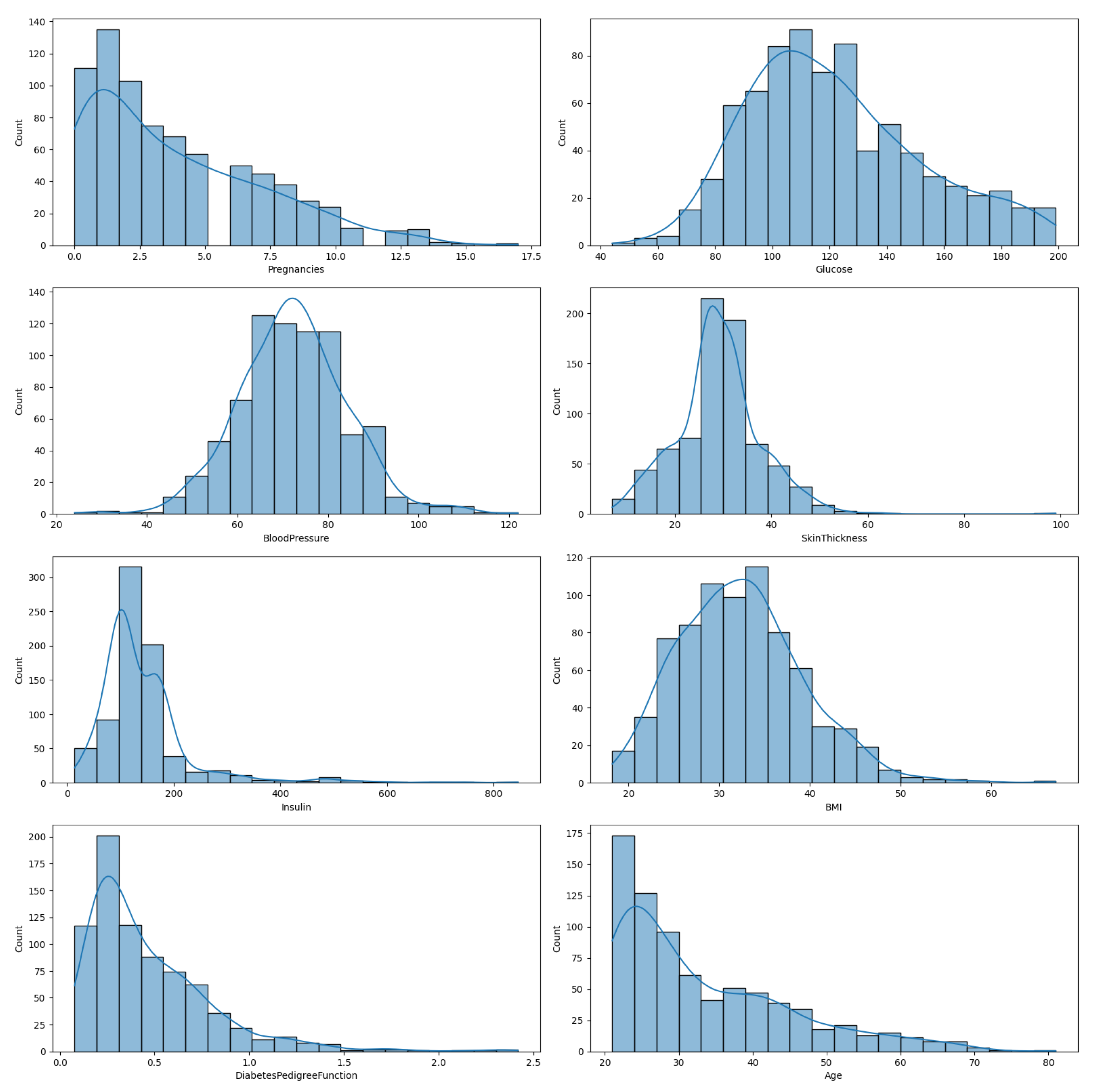
In Figure 1, we illustrate the distribution of the eight features in the diabetes dataset, enabling a comprehensive understanding of each feature’s variability and distribution. This is an important preliminary step before any further statistical analysis or application of ML algorithms.

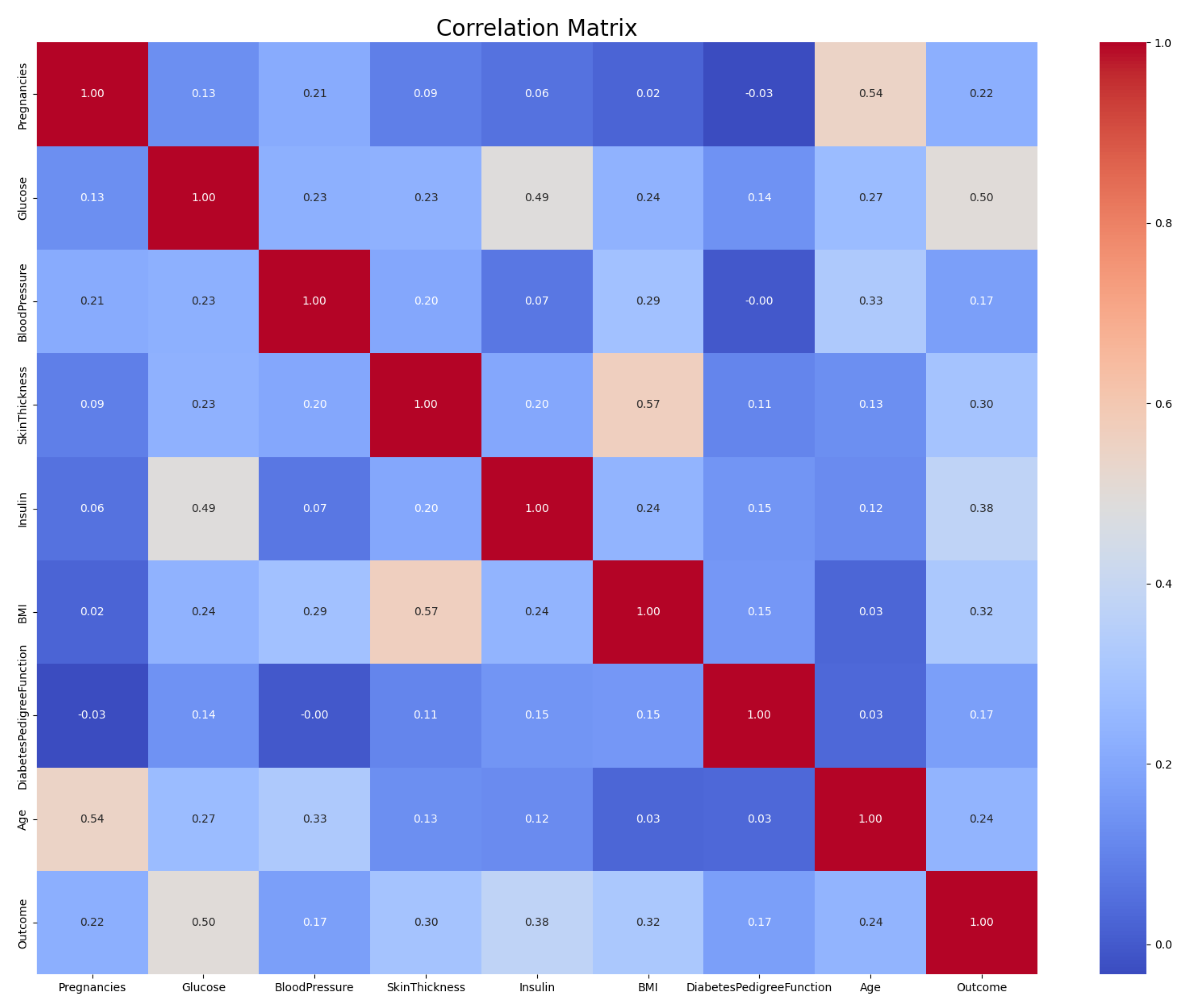
The relationships between the predictors within the dataset are explored in detail in the correlation matrix heatmap depicted in Figure 2. This heatmap provides an understanding of how each predictor variable relates to others, which is essential in understanding complex interdependencies in our model.

In conclusion, while the choice of algorithms and tuning parameters can significantly influence a model’s performance, data curation could be the most important step in a ML pipeline. By carefully handling missing data, we can drastically improve a model’s accuracy, turning a good model into an excellent one.

3.6. Evaluation and ROC Curve

In our study, we leverage an ensemble of DL models to predict disease outcomes, using a two-tiered architecture. The performance of our models is evaluated using the receiver operating characteristic (ROC) curve, a graphical plot that depicts the diagnostic ability of a binary classifier.

First, we generate averaged probabilities for the initial set of ensemble networks. After training, each model generates a set of softmax probabilities for the outcomes, which we average across all models. The initial set of predictions is then used as input to train a secondary set of ensemble networks, following the same procedure as above. The secondary ensemble, known as SuperNet, has a similar architecture but is specifically designed to handle the higher dimensional input from the first stage.

Table 6. Initial Ensemble Classification Report.

	Precision	Recall	F1-Score	Support
0	0.93	0.85	0.89	297
1	0.76	0.88	0.82	164
Accuracy		0.86	461
Macro Avg	0.84	0.86	0.85	461
Weighted Avg	0.87	0.86	0.86	461

presents the classification report for the initial ensemble, offering insight into the precision, recall, and F1-score for each class, along with overall accuracy, macro average, and weighted average metrics. The confusion matrix for the initial ensemble is provided in

Table 7. Initial Ensemble Confusion Matrix.

	Predicted: 0	Predicted: 1
Actual: 0	251	46
Actual: 1	19	145

, illustrating the distribution of actual and predicted classes.

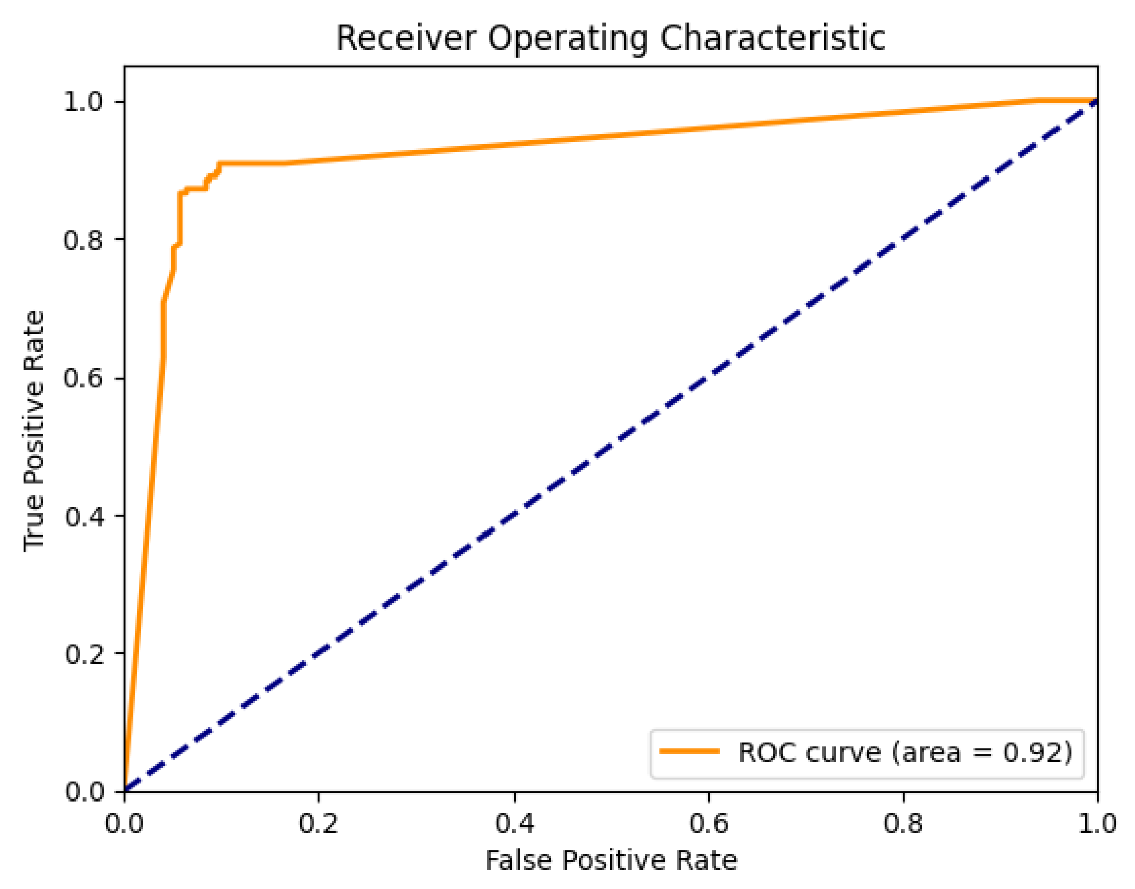
Once the secondary ensemble models are trained, they generate another set of softmax probabilities for the outcomes. These probabilities are again averaged across all models and form the basis for a second ROC curve; as seen in Figure 3. This two-tiered, or ’stacked’, model architecture allows us to increase the complexity and performance of our model without overfitting, as the SuperNet is learning from the predictions of multiple models instead of raw data.

As illustrated in

Table 8. Detailed classification metrics showing the model’s precision, recall, F1-score and support for each class, along with overall accuracy, macro average, and weighted average metrics.

	Precision	Recall	F1-Score	Support
0	0.93	0.94	0.93	297
1	0.88	0.87	0.88	164
Accuracy		0.91	461
Macro Avg	0.91	0.90	0.91	461
Weighted Avg	0.91	0.91	0.91	461

, the model exhibits an overall accuracy of 91%. Further inspection of

Table 9. Confusion matrix representing the distribution of actual and predicted classes, allowing for the visualization of true positives, true negatives, false positives, and false negatives.

	Predicted: 0	Predicted: 1
Actual: 0	278	19
Actual: 1	21	143

reveals that the model achieved a high rate of true positives and true negatives, while keeping the false positives and false negatives relatively low.

As can be seen, stacking our ensemble models significantly improved the accuracy, while also reducing the number of false positives and false negatives.

3.7. Predictor Importance Evaluation and Sensitivity Analysis

Understanding the relative influence of each predictor on the outcomes of a machine learning model is a key aspect of model interpretability and transparency. To shed light on the extent to which each variable contributes to our predictions, we performed a sensitivity analysis. This approach, originally proposed by Saltelli et al. [18], allows us to assess how the variance in our model’s output can be attributed to variations in its inputs.

In our study, the sensitivity analysis was conducted on one model within the first ensemble, see

Table 10. Indices First-Order Sobol and Total-Order for each predictor in the initial diabetes-prediction model. This analysis was executed on the inaugural network within the ensemble, prior to the implementation of cascading. A thorough examination of predictor influence in later ensemble stages poses greater complexity due to the dimensionality increase in the SuperNet architecture—from the original eight attributes to a 100-dimensional space corresponding to the size of the primary ensemble. Hence, interpretability is inherently more challenging in these subsequent stages.

Predictor	First-Order Index Sobol	Total-Order Index Sobol
Pregnancies	0.04393478	0.04300161
Glucose	0.04792455	0.04966603
BloodPressure	0.1176754	0.11754018
SkinThickness	0.39438682	0.39478155
Insulin	0.09117344	0.09335395
BMI	0.10445807	0.10289758
DiabetesPedigreeFunction	0.1756332	0.17328341
Age	0.02469845	0.02507718

, before executing the cascading process. This selection was made to simplify the interpretation of the analysis, as elucidating the complex interactions within the cascaded ensemble would pose significant challenges.

The results of the sensitivity analysis reveal that ‘SkinThickness’ holds the highest degree of influence on the model’s output, as evidenced by its highest first-order and total-order Sobol indices. This suggests that variations in ‘SkinThickness’ could significantly influence the model’s diabetes predictions. Conversely, ‘Age’ appears to have the least impact on the output variance, suggesting a lesser role in the prediction process.

It is important to note that these results only provide a relative measure of each predictor’s contribution and does not inform on the nature (positive or negative) of the relationship between the predictor and the outcome.

The inclusion of this sensitivity analysis in our study not only improves the interpretability of our model, but it also offers potential insights into the critical factors affecting diabetes, furthering our understanding of this complex disease.

4. Discussion

The results obtained in this research clearly indicate the advantage of using cascading and ensemble techniques in improving the predictive capabilities of DL models. The accuracy improvement achieved by integrating bagging, boosting, stacking, and cascading techniques in a predictive system confirms the hypothesis that model diversity in an ensemble leads to better generalization. While our initial model using simple feed-forward networks achieved a modest accuracy, the application of ensemble methods provided significant improvements. Bagging and boosting, being rather straightforward ensemble approaches, already resulted in better predictive performance. Stacking, which involves using the predictions of base models as input to another model, offered further improvement, demonstrating the value of model layering.

The most remarkable improvement was observed with the use of cascading, a technique that extends stacking by training each model on the outputs of all previous models. This method allowed for a more expressive and potent ensemble, as later models could learn complex, high-level patterns from the predictions of earlier models. One important factor in our research was the use of DL models, allowing for non-linear and complex decision boundaries, which seemed particularly suitable for our task.

In our ensemble approach, we harness the strength of multiple individual models and aggregate their predictions to improve accuracy. The scientific basis of this strategy lies in the concept of ‘wisdom of the crowd’. Multiple weak learners, when combined, can outperform a strong learner by compensating for each other’s errors. This approach reduces the model variance without increasing the bias, leading to more robust and reliable predictions. Furthermore, cascading enhances this process by adding a hierarchical structure where the output of one level of models serves as input to the next. This hierarchical processing allows us to capture complex, high-level features from the data, enhancing our model’s discriminatory power. In terms of explainability, each individual model in our ensemble and cascade contributes to the final prediction. By examining the predictions of individual models, we can gain insights into the data features that are most influential in driving the outcomes. Although our model involves sophisticated techniques, its operation can still be understood by dissecting it into its constituent models. Future work could focus on improving the explainability of our model further, aiming to provide clear interpretations of its internal decision-making process.

However, while our ensemble methods have demonstrated their effectiveness, it is important to note that they also introduce additional computational cost and complexity. Depending on the available resources and the problem at hand, this increase might be a limiting factor. Moreover, while our cascading ensemble has shown good results, it may not be the optimal solution for all tasks. The structure of the cascading ensemble, especially the number and arrangement of layers, is an additional hyperparameter that needs to be tuned and may depend on the specifics of the dataset.

In this study, our focus has been to optimize the model’s performance on a well-known diabetes dataset from Kaggle, with an ultimate goal of achieving state-of-the-art model accuracy. Our choice of this dataset is rooted in its wide acceptance and usage in the data science community for benchmarking and comparison purposes. Nevertheless, we understand the significance of testing the developed models on additional datasets to verify their robustness and generalizability. While we have emphasized performance improvements in this work, we acknowledge the importance of broader validation. In future work, we could apply our model to other diabetes datasets and undertake a more comprehensive analysis to assess its adaptability and versatility across various problem settings and data characteristics.

Additionally, climate patterns have been shown to correlate with lifestyle behaviors, disease patterns, and other environmental determinants of health. It is important to mention that the complexity of health data often presents intricate temporal patterns, comparable to those observed in climate data. Therefore, the techniques employed for temperature time-series analysis, such as addressing trend, seasonality, heteroscedasticity, and noise, could also be valuable when dealing with health data. Time-series analysis could potentially offer a rich set of analytical skills applicable to intricate health datasets, should they exhibit temporal patterns.

While we have chosen to prioritize the exploration of ensemble and cascading DL models for the prediction of diabetes in this study, we believe that the integration of time-series analysis could be a fascinating direction for future research. The fusion of traditional classification models with time-series prediction techniques could potentially give rise to more robust models, capable of capturing temporal dependencies in the data.

5. Conclusions and Future Work

In this paper, we explored the use of ensemble techniques in DL, particularly in predicting diabetes onset. Starting from the use of simple feed-forward networks, we progressively introduced bagging, boosting, and stacking techniques. However, the most significant improvement in predictive accuracy was achieved through the implementation of cascading techniques in our ensemble architecture. The achieved results confirmed our initial hypothesis that model diversity within an ensemble leads to better generalization and thus higher predictive accuracy. This understanding provides a valuable contribution to the body of knowledge in the field of predictive modeling in healthcare, particularly in the prediction of diabetes.

The study underscored the potency and practicality of our proposed techniques, which yielded a compelling accuracy of 91.5% on the test set in a very challenging dataset for diagnostic of diabetes. The comprehensive comparison conducted against several other methodologies, confirmed the good performance of our technique. This study has emphasized the significant role that data curation and preprocessing play in the development and effectiveness of ML models. As demonstrated, accurate identification and sophisticated handling of missing values have led to a considerable improvement in our models’ performance. Therefore, investing in meticulous data curation can be a key to achieving high-performing models.

Despite the promising results, this research is not without limitations, the most significant being the increased computational cost and complexity associated with the ensemble methods. Future studies could explore techniques to reduce the computational cost without a significant impact on predictive accuracy. Future work could also extend the application of these ensemble techniques to other healthcare-related problems, as well as explore different configurations of the cascading ensemble. Additionally, investigating methods for automatic tuning of the cascading ensemble architecture could be a fruitful area of research.

As further work, we also see a valuable opportunity to enrich our diabetes-prediction pipeline by integrating time-series analysis into our modeling approach. By leveraging the temporal patterns inherent in healthcare data, such as the progression of vital signs and blood-sugar levels over time, we could potentially improve the sensitivity of our model and provide more personalized risk assessments. This approach could also accommodate the dynamic nature of health status, reflecting more accurately the progression of conditions like diabetes. Thus, the integration of time-series analysis into our existing framework represents a promising avenue for future research.