Trajectory Tracking Control of Autonomous Vehicles Based on an Improved Sliding Mode Control Scheme

Abstract

This paper addresses the issue of external unknown environmental interference affecting the trajectory tracking performance and driving stability of autonomous vehicles. This seriously impacts the performance and stability of the vehicle while driving. In order to provide precise, reliable, and safe trajectory tracking performance for autonomous vehicles, this paper proposes a recursive integral terminal sliding mode control (RITSMC) method. The proposed RITSMC combines the advantages of recursive integral sliding mode (RISM), terminal sliding mode (TSM), and adaptive algorithms, and can effectively achieve precise trajectory tracking and driving stability of autonomous vehicles. Furthermore, compared with traditional methods, an adaptive algorithm is introduced on the recursive sliding surface to enable real-time adaptation of the control parameters of the recursive controller, further improving the trajectory tracking accuracy and driving stability of autonomous vehicles. The stability of this control system is demonstrated by using a Lyapunov function. Finally, multiple simulation tests were conducted on different lane speeds on both wet and dry asphalt road sections. By comparing the simulation results, it was found that the proposed RITSMC exhibits excellent performance in terms of the precision of tracking trajectories and the stability of driving, in contrast to traditional sliding mode controllers (SMC) and integral terminal sliding mode controllers (ITSMC).

1. Introduction

In the era of intelligence, advanced technologies such as data analytics, sensors, and AI technologies have provided new opportunities for the development of autonomous vehicles [1]. Therefore, automated driving technology, which encompasses multidisciplinary theories and methods, has become a current research hotspot [2]. Autonomous vehicles possess precise trajectory tracking capabilities, thereby significantly alleviating road congestion [3]. Furthermore, autonomous vehicles exhibit excellent lateral stability, further enhancing passenger safety and comfort [4]. However, in real-world driving environments, numerous unknown external interferences exist. Due to the sensitivity of autonomous vehicles to these interferences, the accuracy of road tracking and driving stability are affected. Therefore, it is crucial to suppress the impact of external interferences on autonomous vehicles and enhance the performance of autonomous driving systems.

Trajectory tracking is a crucial aspect of autonomous driving technology [5]. Its purpose is to ensure that the vehicle follows the desired trajectory with minimal deviation, given the specified desired trajectory. Currently, there are many relevant studies emerging in the domain of autonomous driving. Lu et al. [6] put forward an improved RRT algorithm, which converts the target point into a random point to expand the random tree and achieve trajectory tracking of autonomous vehicles within the road boundary. Nevertheless, the algorithm exhibits a slow convergence rate and significant path fluctuations. Hence, Yang et al. [7] proposed a control method based on Model Predictive Control (MPC) and Fuzzy Proportional–Integral–Derivative (PID) for precise control of the steering angle by applying MPC to the lateral controller. Additionally, a fuzzy PID is utilized to configure the longitudinal controller in order to reduce the lateral error, thereby improving the vehicle’s trajectory tracking accuracy. Liu et al. [8] proposed a reinforcement learning approach to achieve trajectory tracking for autonomous vehicles. The method uses reinforcement learning to conduct tracking experiments on extracted driving scenarios and road information, thus ensuring the stability and trajectory tracking accuracy of autonomous vehicles. The aforementioned algorithms have, to some extent, improved the accuracy of autonomous vehicles in tracking the reference path. However, due to the slow convergence speed of these algorithms, the adaptability of vehicles to environmental changes is severely affected, reducing the real-time capability of the system. Zuo et al. [9] suggested a model predictive control (MPC) method based on an improved particle swarm optimization algorithm (IPSO) to solve the trajectory tracking problem by treating time-varying safety constraints as a repulsive range and an asymmetric lane potential field function, thereby obtaining collision-free paths to ensure accurate vehicle trajectory tracking. Nie et al. [10] proposed an autonomous vehicle trajectory tracking system that fully considers the road friction issue. They employed the Variable Forgetting Factor Recursive Least Squares (VFF-RLS) method to identify the road adhesion coefficient, which was then fed into the Model Predictive Control (MPC) to enhance the slip angle constraint and improve trajectory tracking accuracy. Huang et al. [11] proposed a Human–Machine Cooperative Rapid Random Tree (HM-RRT) algorithm, which combines driver behavior assessment and the driver’s anticipated tasks to generate collaborative trajectories through the newly developed HM-RRT. By incorporating driver intentions and automated corrective measures, the algorithm aims to improve the trajectory tracking accuracy of the vehicle. However, while these algorithms improve tracking accuracy and convergence speed, they also increase the computational complexity of the system, posing challenges to the real-time capability and practicality of autonomous driving systems. Furthermore, a single simulation environment has limitations and cannot simulate various complex real-world scenarios, which restricts the adaptability and reliability of the algorithms.

As the trajectory tracking technology of autonomous vehicles continues to develop, researchers have begun to combine trajectory tracking with lateral stability [12]. The main goal of this technology is to ensure that autonomous vehicles maintain lateral stability while achieving precise trajectory tracking, thus preventing deviations from the trajectory or loss of control [13]. Huang et al. [14] proposed a lateral stability control method based on a combination of movable regions and stable controllers. They designed a dynamic sliding mode controller based on the characteristics of stable region movement and dynamic margin to keep the vehicle driving in the stable region. Cheng et al. [15] proposed a lateral stability control system based on the model predictive controller (MPC), which calculates the required yaw moment and tire forces to maintain the lateral stability of the vehicle. The aforementioned literature describes research on the lateral stability of autonomous driving systems, which ensures their lateral stability when based on stable regions. However, in actual driving scenarios, these systems are prone to being influenced by complex environments, making it difficult to guarantee the lateral stability of the vehicle. He et al. [16] proposed an inverse sliding mode control algorithm to enable autonomous vehicles to track reference paths effectively and ensure lateral stability during driving. However, this controller is unable to perform effective trajectory tracking in complex environments and tends to have long settling times, leading to phenomena such as oscillations. Sliding mode control, as a classic nonlinear control strategy [17], can generate discontinuous control to force the driving system to move along the reference trajectory. Simultaneously, the sliding mode controller possesses benefits, including rapid response, high precision, and robustness. However, traditional sliding mode controllers (SMC) exhibit a chattering phenomenon after the system state reaches the sliding surface [18], which affects control accuracy and system stability. To address this issue, researchers have proposed various methods, among which terminal sliding mode control (TSM) [19] is a commonly used approach. Compared with traditional sliding mode control, TSM cannot only suppress chattering but also shorten the convergence time. However, this control method can cause singularity problems. To avoid the singularity problem, researchers proposed non-singular terminal sliding mode control (NTSMC) [20], which has a slow response and cannot effectively deal with complex scenarios. To improve the response speed of the controller, researchers proposed a recursive terminal sliding mode control [21], but this method cannot converge to zero gradually in complex environments. To improve the convergence performance of the control system, researchers have proposed an adaptive SMC control method [22], which can adapt to complex environments. However, it relies heavily on the robustness of the system and has a large computational cost. In recent years, the Integral Terminal Sliding Mode Control (ITSMC) [23] has been proposed, which not only guarantees finite-time convergence, but also accelerates the convergence speed. Based on the various sliding mode control methods introduced in the aforementioned literature, it can be observed that single-mode sliding control suffers from drawbacks such as slow response speed, low adaptability to complex environments, and strong oscillations. Therefore, it is highly necessary to design an optimized sliding mode controller.

Based on the aforementioned literature, it is evident that significant progress has been made in autonomous driving technology. However, there are still some areas for optimization identified in the literature. We summarize these optimization areas as follows: (1) Some researchers have focused excessively on autonomous driving trajectory tracking based on stable regions, neglecting the impact of external interferences on vehicles in real driving environments, thereby compromising the performance of the control system. (2) Most simulation validation work has been conducted on fixed road segments, overlooking the influence of various complex road segments in actual driving environments on trajectory tracking accuracy and stability. (3) Researchers have emphasized improving path tracking accuracy and stability while overlooking the computational complexity of the system, leading to issues such as delayed system response and decreased reliability. Therefore, further optimization of the control system is necessary. (4) Sliding mode control is mentioned in the literature for its robustness and high accuracy. However, single-mode sliding control has various drawbacks that make it difficult to address the challenges faced by autonomous driving vehicles in practice. Hence, there is a need to optimize control algorithms to further enhance the robustness and reliability of autonomous driving systems in diverse driving environments.

Based on the summary of the aforementioned literature, this paper provides a detailed supplement to the areas for optimization. Firstly, we introduce an external disturbance term based on previous research to investigate the stability of autonomous driving vehicles. The application of this method accurately simulates the uncertainty factors in actual driving environments, overcoming the limitations of previous studies based on stable regions and better evaluating the stability of autonomous driving vehicles in real driving scenarios. Secondly, in order to comprehensively consider the influence of actual driving environments on trajectory tracking accuracy and stability, we design multiple simulation environments, including various road structures and different road conditions. By using these diverse environments for simulation, we overcome the limitations of a single environment and more accurately reflect the performance of the autonomous driving system in different driving scenarios. Finally, the proposed method employs a recursive sliding mode surface design combined with an adaptive algorithm, significantly improving the system’s disturbance rejection capability while reducing complexity and computational load. This algorithm can dynamically adjust the sliding mode control parameters in real-time, enhancing the system’s adaptability to disturbances. Moreover, the adoption of exponential convergence law strengthens the convergence performance, ensuring the system reaches a stable state within a finite time. These improvements effectively enhance the robustness and control accuracy of the autonomous driving system. The practical significance of this paper lies in addressing the issue of external disturbances faced by autonomous driving systems in real driving environments, providing important references for the development of more reliable autonomous vehicles. The introduction of external disturbance terms, diverse simulation environments, recursive sliding mode surfaces, and adaptive algorithms enables the autonomous driving system to adapt to various complex and dynamic driving conditions. The proposed method establishes a solid foundation for the application of autonomous driving vehicles in practical scenarios.

In conclusion, this paper proposes a recursive integral terminal sliding mode controller. The main contributions of this study can be summarized as follows:

(1) This paper utilizes an integral terminal sliding mode surface to improve upon the traditional non-singular terminal sliding mode surface, effectively suppressing external disturbances and enhancing the system’s disturbance rejection capability.

(2) This paper employs an exponential reaching law to enhance the stability and disturbance rejection of the system, surpassing the performance of the power reaching law. It enables adaptability to various diverse driving environments.

(3) This paper proposes an adaptive algorithm for online adjustment of the error control parameters, the error power integration control parameters, and the recursive control parameters on the integral terminal sliding mode surface. This method enhances the adaptability of intelligent control systems to external environments and reduces the system complexity.

(4) By incorporating disturbance terms, it enables the accurate simulation of more realistic driving environments, which aids in verifying and improving the stability, robustness, and safety of the autonomous driving systems.

Finally, multiple experiments were conducted based on Simulink-Carsim co-simulation in various lanes, different speeds, and different road sections to verify the designed controller’s ability to control the vehicle’s trajectory tracking accuracy and stability.

2. Constructing a System Model

The construction of a model is an important basis for studying the controlled object. In this paper, a controlled object model combining a two-degree-of-freedom (2DOF) vehicle dynamic model with a kinematic model will be constructed to better describe the state variables of autonomous vehicles. Additionally, the definitions of the symbols can be found in

Table 1. List of symbols.

Symbol	Parameters
$F_{fl}$, $F_{fr}$	Lateral force of the left and right tires of the front axle of the vehicle
$F_{rl}$, $F_{rr}$	Lateral force of the left and right rear axle tires of the vehicle
$\beta$	Vehicle sideslip angle
$\gamma$	Vehicle yaw angle speed
$m$	Total vehicle mass
$I_z$	Yaw moment of inertia
$v_x,{\mathrm{v}}_{\mathrm{y}}$	Transverse and longitudinal speed of vehicle
$a$,$b$	The distance between the center of gravity of the vehicle and the front and rear axles
$e$	Lateral error
$\psi$	Heading error
$e_m$	Mapping error
${\delta }_f$	Front wheel angle
$x_m$	Constant projection distance
$d$	The distance traveled by the vehicle along the reference path
$\varphi$, ${\varphi }_r$	Vehicle heading angle and reference path heading angle
${\dot{v}}_x,{\dot{v}}_y$	Transverse and longitudinal acceleration of the vehicle
$\rho$	Path curvature
$k_1,k_2$	Front and rear axle lateral stiffness of vehicle
${\alpha }_r$	Vehicle rear axle side deflection angle

in this paper.

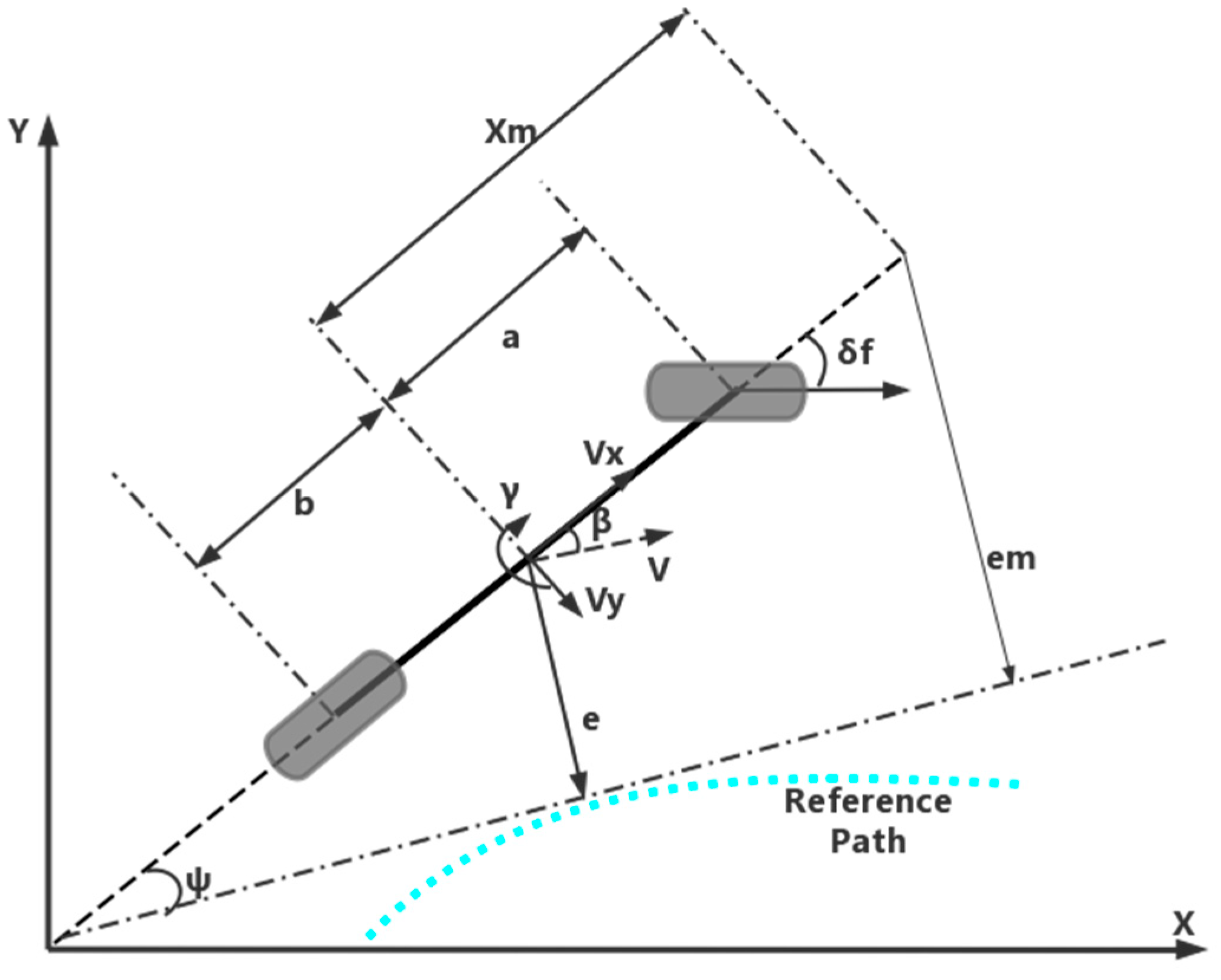
2.1. Vehicle Dynamics Model

Constructing a model that accurately represents the lateral dynamic characteristics of a vehicle is highly significant for studying the trajectory tracking of autonomous vehicles. In this paper, a 2DOF vehicle dynamic model [24] is constructed:

$$\left\{\begin{array}{c}\dot{\beta }=\frac{F_{fl}+F_{fr}+F_{rl}+F_{rr}}{m{v}_x}-\gamma \\ \dot{\gamma }=\frac{a\left(F_{fl}+F_{fr}\right)-b(F_{rl}+F_{rr})}{I_z}\end{array}\right.$$

(1)

As the vehicle passes through different road sections at different speeds, this can cause the sideslip angle and yaw rate of the vehicle to become too large or too small, resulting in a loss of vehicle stability.

2.2. Vehicle Kinematic Model

To enhance the path tracking capability of autonomous vehicles, the state variables of vehicle dynamics are transformed into state variables related to the trajectory tracking path, and a model schematic as shown in Figure 1 is constructed:

If the vehicle is driving at high speed on a low-friction-coefficient road surface, the stability of the vehicle will decrease, and the mapping error will also change, thereby affecting the accuracy of the vehicle’s path tracking. Figure 1 depicts the vehicle kinematic model [25]:

$$\left\{\begin{array}{l}{e}_m=e+x_m\mathit{sin}\left(\psi \right)\\ \dot{e}=v_x\mathit{sin}\left(\psi \right)+v_{y}cos(\psi )\\ \dot{d}=v_x\mathit{cos}\left(\psi \right)-v_{y}sin(\psi )\\ \psi =\varphi -{\varphi }_r\end{array}\right.$$

(2)

Based on Equations (1) and (2), the expression for the mapping error can be obtained as follows:

$$\left\{\begin{array}{l}{\ddot{e}}_m=w_1+w_2+w_3{\delta }_f+d_e\\ w_1={\dot{v}}_y+{\dot{v}}_x\psi +v_x(\gamma -\rho \dot{d})\\ w_2=x_m[\frac{a(v_x\beta +a\gamma )k_1}{v_x{I}_z}-\frac{b{\alpha }_r{k}_2}{I_z}-\dot{\rho }\dot{d}-\rho \ddot{d}]\\ w_3=-x_m\frac{a{k}_1}{I_z}\end{array}\right.$$

(3)

where $d_e$ represents disturbance uncertainty and satisfies the following relationship:

$$\left|d_e\right|\le D$$

(4)

where $D$ is a constant greater than zero, representing the upper bound of the disturbance uncertainty.

Accordingly, the expression with disturbance uncertainty can be ultimately represented as:

$$\left\{\begin{array}{l}{\dot{x}}_1=x_2\\ {\dot{x}}_2=w_1+w_2+w_{3}u+d_e\end{array}\right.$$

(5)

where $x_1=e_m$; $u={\delta }_f$ represents the vehicle’s steering angle of the front wheels. ${\delta }_f$ is also the input signal of the closed-loop system. With the increase in vehicle speed, the road adhesion coefficient decreases, and some unfavorable phenomena such as deviation from the reference path and vehicle body shaking will occur in autonomous driving vehicles. This will lead to energy waste and economic losses. Therefore, when designing controllers, we should eliminate these adverse factors that are present, so that the vehicle has higher tracking accuracy and stronger stability.

3. Controller Design

This section aims to address the issues of trajectory tracking accuracy and lateral motion stability that autonomous vehicles may face while driving in complex road conditions, often caused by external unknown disturbances. Therefore, this paper proposes a solution based on the RITSMC.

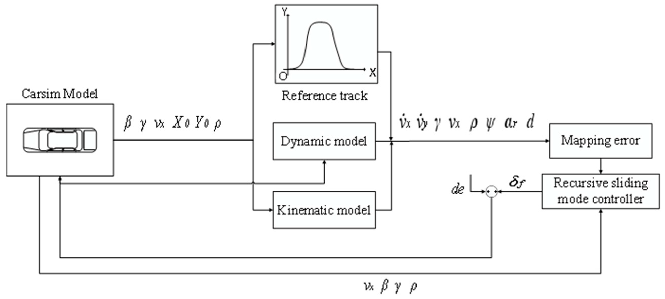
3.1. Controller Structure

The RITSMC closed-loop control system is depicted in Figure 2. In order to verify that this controller has good control performance, we adopted a form of joint simulation using Matlab and Carsim and built a high-fidelity vehicle simulation model on the platform for simulation verification. This can effectively simulate the driving situation of autonomous vehicles on real roads and obtain accurate and reliable data, further analyzing the performance and stability of the proposed controller.

3.2. Design of Control Law

The reference signal $x_r$ and the tracking error $e$ of the control system are defined based on the aggregated model described in Equation (5):

$$\left\{\begin{array}{l}{x}_r=0\\ e=x_1-x_r=x_1\\ \dot{e}={\dot{x}}_1-{\dot{x}}_r=x_2\end{array}\right.$$

(6)

First, we define the RITSM function as follows:

$$s=\sigma +\lambda {\sigma }_I$$

(7)

where the ITSM function $\sigma$ is defined as:

$$\left\{\begin{array}{l}\sigma =\dot{e}+{\widehat{\lambda }}_1+{\widehat{\lambda }}_2{\int }_0^t{e}^{\frac{q}{p}}{d}_{\tau }\\ {\sigma }_I={\left|\sigma \right|}^{{\epsilon }_3}sign(\sigma )\end{array}\right.$$

(8)

where ${\epsilon }_3>1; p,q$ are positive odd integers; the initial value ${\sigma }_I(0)=-1/{\widehat{\lambda }}_3(0)[\dot{e}(0)+{\widehat{\lambda }}_1(0)e(0)+{\widehat{\lambda }}_2(0){\int }_0^t{e}^{\frac{q}{p}}(0)d_{\tau }]; {\widehat{\lambda }}_1, {\widehat{\lambda }}_2, {\widehat{\lambda }}_3$ represent the expression for updating the variable parameters online in real time using an adaptive law:

$$\left\{\begin{array}{l}{\dot{\widehat{\lambda }}}_1=-{\eta }_{1}se\\ {\dot{\widehat{\lambda }}}_2=-{\eta }_{2}s{\int }_0^t{e}^{\frac{q}{p}}{d}_{\tau }\\ {\dot{\widehat{\lambda }}}_3=-{\eta }_{3}s{\sigma }_I\end{array}\right.$$

(9)

where ${\eta }_1,{\eta }_2, {\eta }_3$ are the positive adaptive gain.

Lemma 1.

According to Equation (5), in order to achieve rapid convergence of the tracking error, the design of the sliding mode control law is as follows:

$$u=-\frac{1}{w_3}[{\epsilon }_{1}sign(s)+{\epsilon }_{2}s+w_1+w_2+{\widehat{\lambda }}_1\dot{e}+{\widehat{\lambda }}_2{e}^{\frac{q}{p}}+{\widehat{\lambda }}_3{\dot{\sigma }}_I]$$

(10)

where ${\epsilon }_1{,\epsilon }_2>0$ are two positive constants that need to be designed; ${\widehat{\lambda }}_1$, ${\widehat{\lambda }}_2$, ${\widehat{\lambda }}_3$ are the terminal sliding mode controller parameter estimated online using Equation (8). To ensure the convergence of the system, the value of ${\epsilon }_1$ must be greater than the upper bound of the disturbance uncertainty $d_e$, i.e.,:

$${\epsilon }_1>D\ge \left|d_e\right|$$

(11)

3.3. Stability Analysis of the Controller

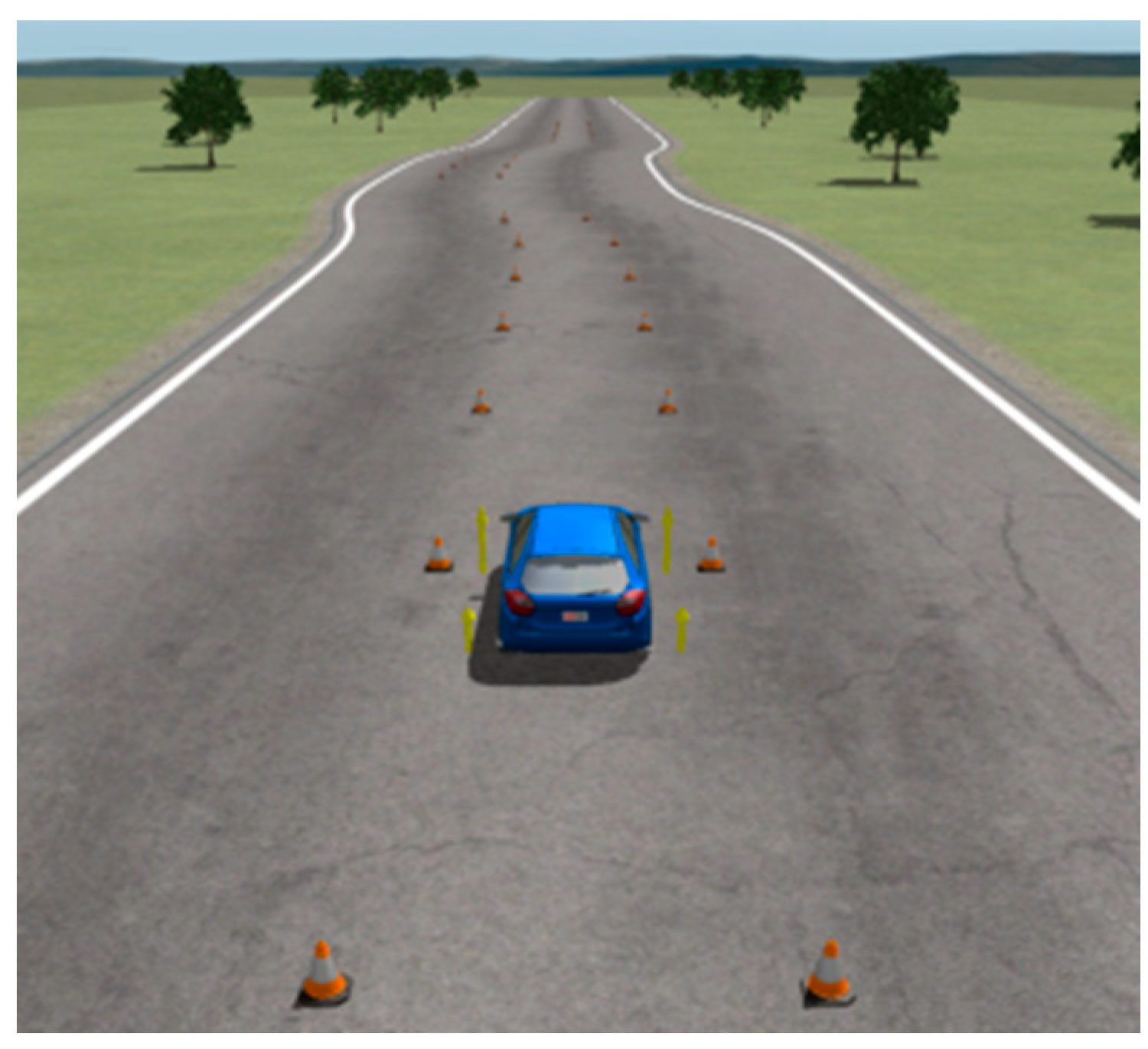
To demonstrate the stability of the controller in Equation (10), a Lyapunov function is designed in this paper as follows:

$$V=\frac{1}{2}{s}^2$$

(12)

$$\begin{gathered} \dot{V}=s\dot{s}=s(\ddot{e}+{\dot{\widehat{\lambda }}}_{1}e+{\widehat{\lambda }}_1\dot{e}+{\dot{\widehat{\lambda }}}_2{\int }_0^t{e}^{\frac{q}{p}}{d}_{\tau }+{\widehat{\lambda }}_2{e}^{\frac{q}{p}}+{\dot{\widehat{\lambda }}}_3{\sigma }_I+{\widehat{\lambda }}_3{\dot{\sigma }}_I)= \\ s[w_1+w_2+w_{3}u+d_e+{\dot{\widehat{\lambda }}}_{1}e+{\widehat{\lambda }}_1\dot{e}+{\dot{\widehat{\lambda }}}_2{\int }_0^t{e}^{\frac{q}{p}}{d}_{\tau }+{\widehat{\lambda }}_2{e}^{\frac{q}{p}}+{\dot{\widehat{\lambda }}}_3{\sigma }_I+{\widehat{\lambda }}_3{\dot{\sigma }}_I] \end{gathered}$$

(13)

Substituting Equation (10) into Equation (13):

$$\begin{gathered} \dot{V}=s[w_1+w_2-({\epsilon }_{1}sign(s)+{\epsilon }_{2}s+w_1+w_2+{\widehat{\lambda }}_1\dot{e}+{\widehat{\lambda }}_2{e}^{\frac{q}{p}}+{\widehat{\lambda }}_3{\dot{\sigma }}_I) \\ +d_e+{\dot{\widehat{\lambda }}}_{1}e+{\widehat{\lambda }}_1\dot{e}+{\dot{\widehat{\lambda }}}_2{\int }_0^t{e}^{\frac{q}{p}}{d}_{\tau }+{\widehat{\lambda }}_2{e}^{\frac{q}{p}}+{\dot{\widehat{\lambda }}}_3{\sigma }_I+{\widehat{\lambda }}_3{\dot{\sigma }}_I] \end{gathered}$$

(14)

The rearranged form of Equation (14) is:

$$\dot{V}=s[-{\epsilon }_{1}sign(s)-{\epsilon }_{2}s+d_e+{\dot{\widehat{\lambda }}}_{1}e+{\dot{\widehat{\lambda }}}_2{\int }_0^t{e}^{\frac{q}{p}}{d}_{\tau }+{\dot{\widehat{\lambda }}}_3{\sigma }_I]$$

(15)

Substituting Equation (9) into Equation (15):

$$\dot{V}=s[d_e-{\eta }_{1}s{e}^2-{\eta }_{2}s{({\int }_0^t{e}^{\frac{q}{p}}{d}_{\tau })}^2-{\eta }_{3}s{{(\sigma }_I)}^2-{\epsilon }_{1}sign(s)-{\epsilon }_{2}s]=s{d}_e-{\epsilon }_1\left|s\right|$$

(16)

Considering the bounded information in Equation (11), we can obtain:

$$\dot{V}\le \left|s\right|(\left|d_e\right|-{\epsilon }_1)<0$$

(17)

Thus, the proof is complete.

During the operation of autonomous vehicles, disturbances from the external environment may cause vehicle shaking in actual driving. To ensure the effectiveness of the adaptive algorithm in estimating time-varying parameter values, we use the following dead-zone correction method to adjust the adaptive process:

$${\dot{\widehat{\lambda }}}_1=\left\{\begin{array}{l}-{\eta }_{1}se,\hspace{1em} for\left|e\right|\ge {\alpha }_e\\ 0,\hspace{1em} \hspace{1em} for\left|e\right|<{\alpha }_e\end{array}\right.$$

(18)

$${\dot{\widehat{\lambda }}}_2=\left\{\begin{array}{l}-{\eta }_{2}s{\int }_0^t{e}^{\frac{q}{p}}{d}_{\tau },\hspace{1em}for\left|e\right|\ge {\alpha }_e\\ 0,\hspace{1em} \hspace{1em} \hspace{1em} \hspace{1em} for\left|e\right|<{\alpha }_e\end{array}\right.$$

(19)

$${\dot{\widehat{\lambda }}}_3=\left\{\begin{array}{l}-{\eta }_{3}s{\sigma }_I,\hspace{1em}for\left|\sigma \right|\ge {\alpha }_{\sigma }\\ 0, \hspace{1em} \hspace{1em} for\left|\sigma \right|<{\alpha }_{\sigma }\end{array}\right.$$

(20)

where ${\alpha }_e>0,{\alpha }_{\sigma }>0$ are positive parameters.

To alleviate the chattering phenomenon caused by the switching function in Equation (10), a boundary layer technique is introduced in this paper to mitigate the effect of chattering on the intelligent controller. Specifically, we use a continuous saturation function to replace the discontinuous switching function, thereby eliminating the instability and oscillations caused by the switching function, as follows:

$$sat(s)=\left\{\begin{array}{l}\frac{s}{\delta },\hspace{1em} \hspace{1em} \hspace{1em} for\left|s\right|<\delta \\ sign(s),\hspace{1em} for\left|s\right|\ge \delta \end{array}\right.$$

(21)

where $\delta >0$ is the boundary layer thickness. When selecting the value of $\delta$, both the tracking accuracy and control stability should be taken into account.

According to Equation (7), by setting an appropriate initial value for ${\sigma }_I$, the sliding variable of the system will start to operate from $s=0$. Based on this favorable characteristic, the approaching process of the sliding variable is omitted, which improves the convergence speed and tracking accuracy of the system. Additionally, the adaptive formula given by Equation (9) can adjust the control parameters online, further enhancing the convergence speed and tracking accuracy of the system.

4. Simulation

Based on the MATLAB and Carsim joint simulation platform, a high-fidelity vehicle model was built to compare the SMC, ITSMC, and RITSMC control methods and analyze the simulation results. The information regarding the vehicle parameters can be found in

Table 2. Vehicle parameters.

Symbol	Value	Parameters
$a/m$	1.015	Distance from the front axis to the center of mass
$\mathrm{b}/\mathrm{m}$	1.895	Distance from the rear axis to the center of mass
${\mathrm{x}}_{\mathrm{m}}/\mathrm{m}$	2.3	Pre-sighting distance
$\mathrm{m}/\mathrm{k}\mathrm{g}$	1416	Vehicle quality
${\mathrm{I}}_{\mathrm{z}}/(\mathrm{k}\mathrm{g}·{\mathrm{m}}^2)$	1536.7	Rotational inertia
${\mathrm{K}}_1/(\mathrm{N}·\mathrm{r}\mathrm{a}\mathrm{d})$	−112,600	Front axle steering stiffness
${\mathrm{K}}_2/(\mathrm{N}·\mathrm{r}\mathrm{a}\mathrm{d})$	−89,500	Rear axle steering stiffness

. To demonstrate that the proposed controller has good stability and tracking accuracy, three operating conditions were designed for simulation comparison analysis in two different road scenarios. Among them, the parameters of the controller can be found in

Table 3. Controller parameters.

Parameter	Value
${\mathsf{\epsilon }}_1$	0.01
${\mathsf{\epsilon }}_2$	25
${\mathsf{\epsilon }}_3$	20
${\mathsf{\eta }}_1$	0.01
${\mathsf{\eta }}_2$	10
${\mathsf{\eta }}_3$	10
${\widehat{\mathrm{k}}}_1(0)$	4
${\widehat{\mathrm{k}}}_2(0)$	0.01
${\widehat{\mathrm{k}}}_3(0)$	1
$\mathrm{p}$	3
$\mathrm{q}$	5
${\mathsf{\alpha }}_{\mathrm{e}}$	0.01
${\mathsf{\alpha }}_{\mathsf{\sigma }}$	2
$\mathsf{\delta }$	0.01

. The first working condition simulates a wet road surface with a set speed of $v=54 \mathrm{k}\mathrm{m}/\mathrm{h}$ and a road adhesion coefficient of $\mu =0.45$. The second scenario simulates a dry asphalt road surface with a set vehicle speed of $v=54 \mathrm{k}\mathrm{m}/\mathrm{h}$ and a road adhesion coefficient of $\mu =0.85$. The third working condition simulates a dry asphalt road surface with a set speed of $v=72 \mathrm{k}\mathrm{m}/\mathrm{h}$ and a road surface friction coefficient of $\mu =0.85$. By comparing the simulation results of these three working conditions, it is possible to reasonably compare the control effects of the three methods under these conditions.

A double lane-change trajectory model was selected as the reference signal for the system, and its simulated driving scenario is shown in Figure 3. The trajectory model can be expressed as follows:

$$\left\{\begin{array}{l}{Y}_r(x)=\frac{d_{n1}}{2}[1+tanh(r_1)]-\frac{d_{n2}}{2}[1+tanh(r_2)]\\ {\varphi }_r=arctan[d_{n1}{(\frac{1}{cosh(r_1)})}^2(\frac{1.2}{d_{m1}})-d_{n1}{(\frac{1}{cosh(r_2)})}^2(\frac{1.2}{d_{m2}})]\end{array}\right.$$

(22)

where $Y_r$, $x$, ${\varphi }_r$ are the reference lateral position, reference longitudinal position, and reference yaw angle of the autonomous vehicle during its driving process, respectively. The selection of the parameter values in the trajectory model is as follows: $r_1=0.096(x-60)-1.2$, $r_2=0.096(x-120)-1.2$, $d_{m1}=25$, $d_{m2}=25$, $d_{n1}=3.6$, $d_{n2}=3.6$.

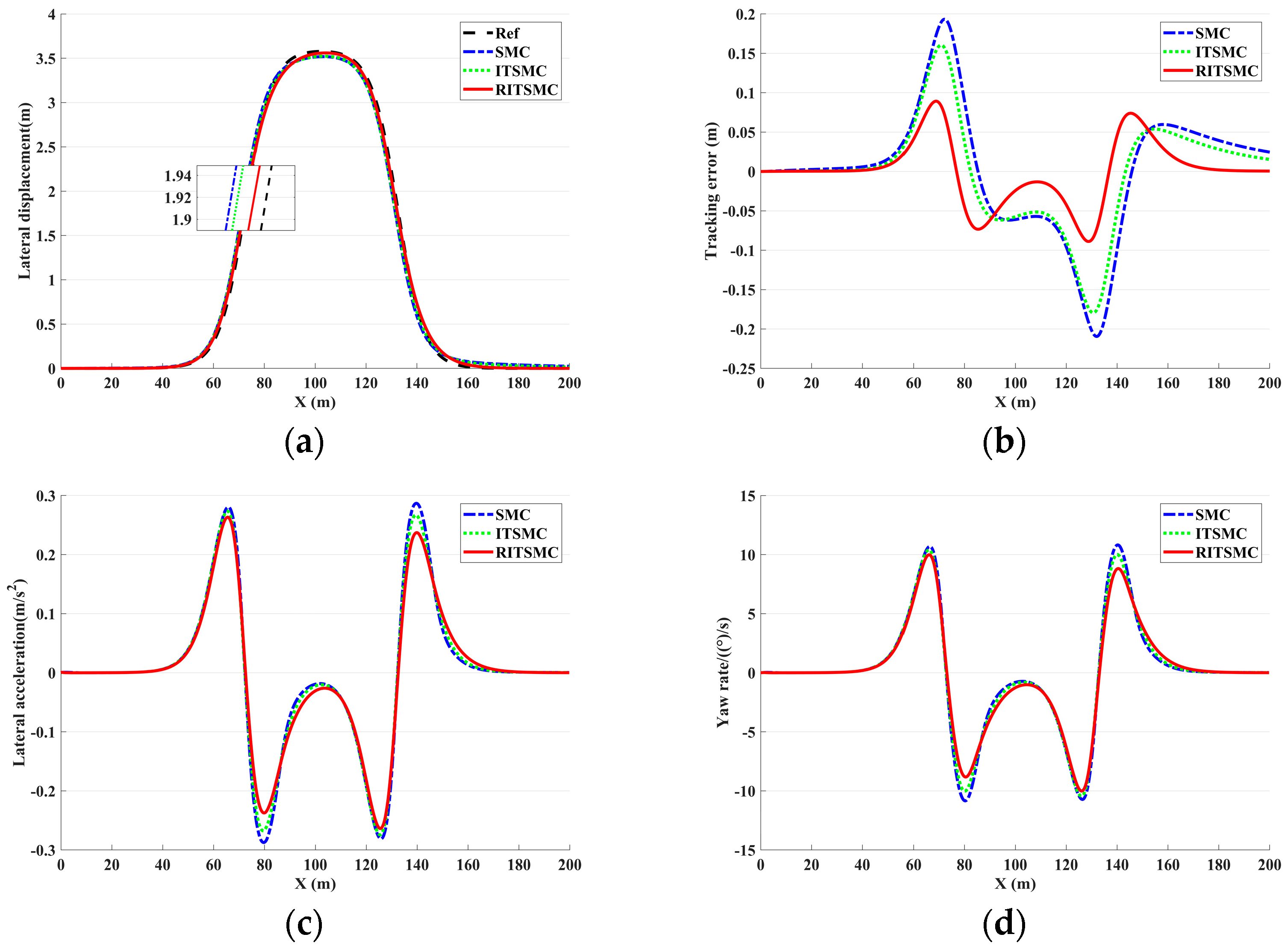
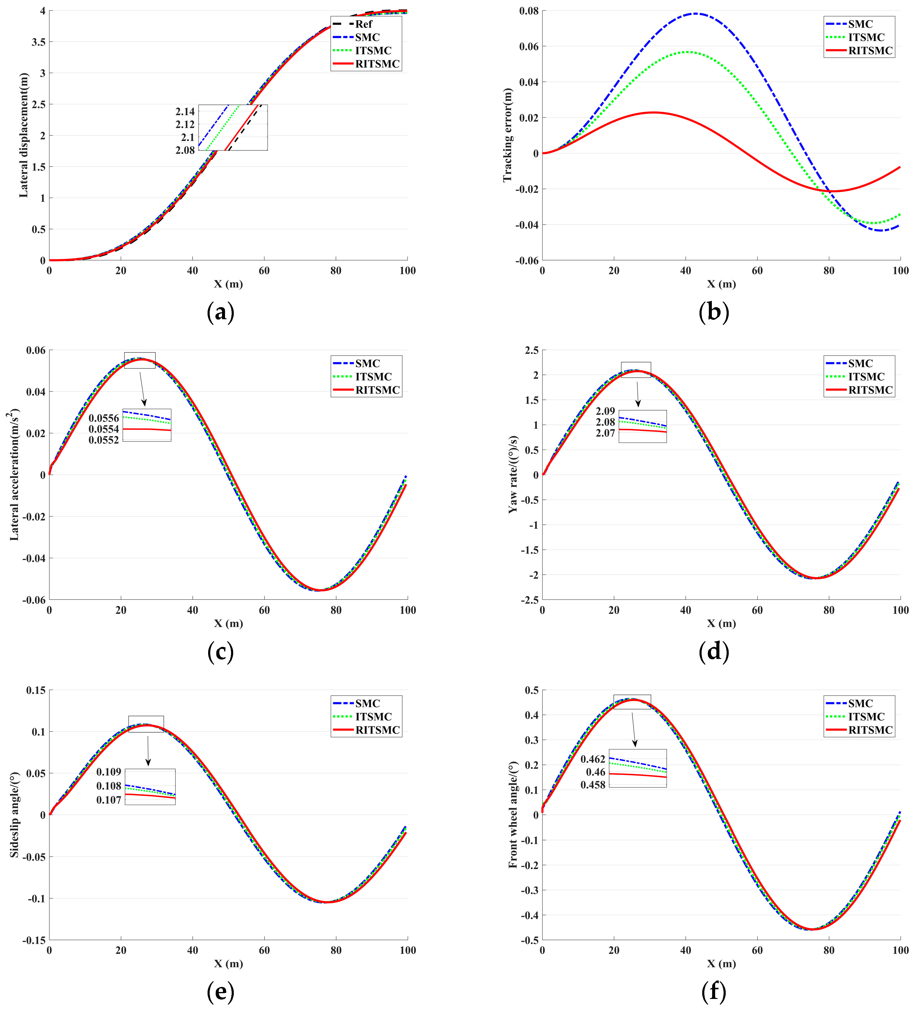
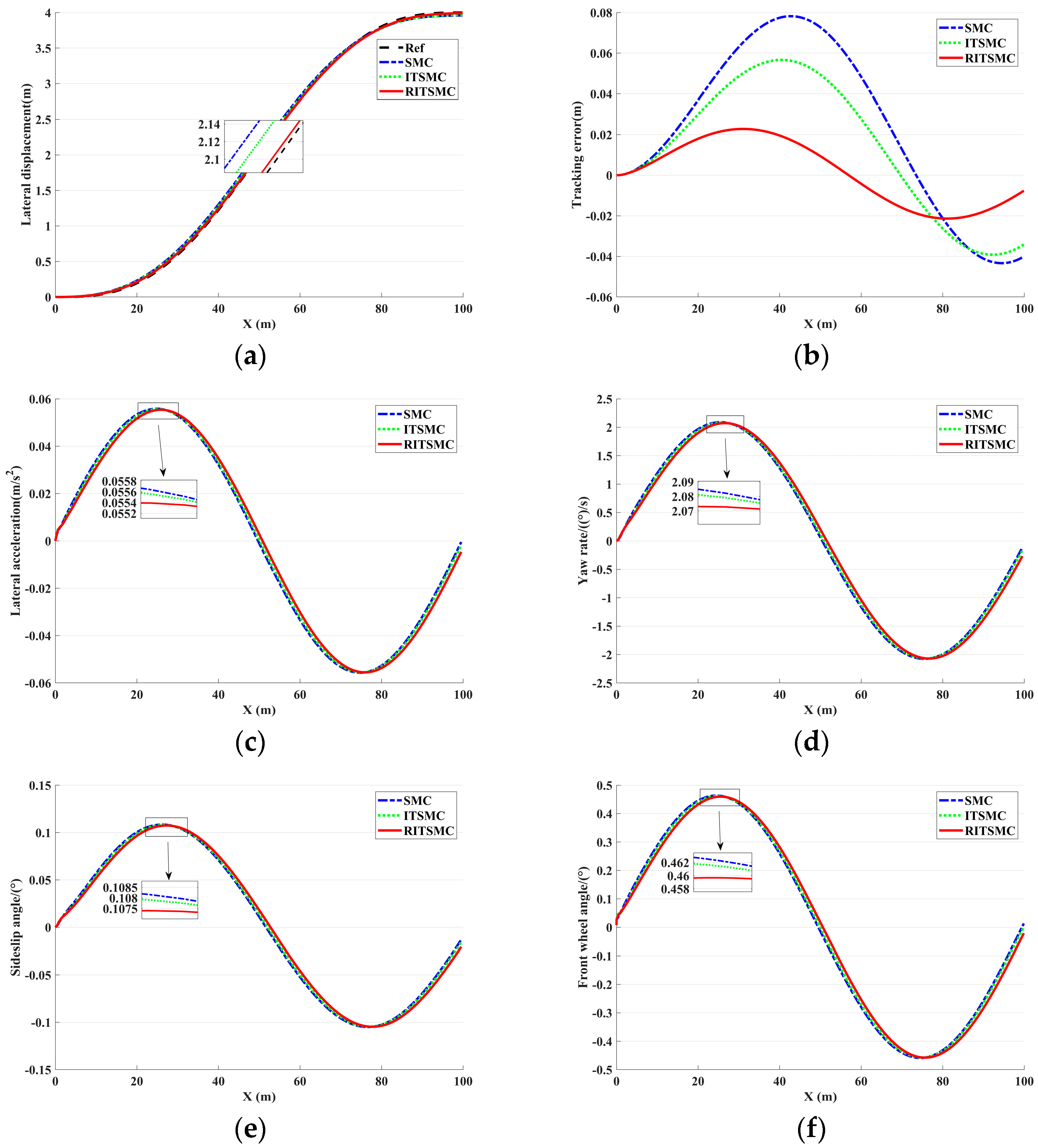
4.1. Double Lane Shift: Comparative Analysis of Controller Effect

4.1.1. Test Condition 1: Low-Speed Wet Road

In this simulation, the effectiveness of RITSMC is tested on a wet road surface, with a set vehicle speed of $v=54 \mathrm{k}\mathrm{m}/\mathrm{h}$ and a ground friction coefficient of $\mu =0.45$.

In Figure 4a, Ref represents the reference trajectory. From the locally magnified image, it can be seen that the actual trajectory generated by the SMC-controlled vehicle has the worst fitting effect with the reference trajectory. According to the simulation results in Figure 4b, it can be observed that the SMC control of the vehicle generates the highest peak of lateral error. This indicates that the algorithm exhibits the poorest trajectory tracking accuracy for the vehicle during the actual driving. In comparison, the actual trajectory generated by the ITSMC-controlled vehicle has a slightly improved fitting effect with the reference trajectory, and its peak value of lateral error is relatively small, as shown in Figure 4b. However, the actual trajectory generated by the RITSMC-controlled vehicle has the best fitting effect with the reference trajectory, and its peak value of lateral error is the smallest compared to SMC and ITSMC. According to

Table 4. Dual moving average peak error table.

Vehicle Speed/Road Grip /(km/h)	SMC/m	ITSMC/m	RITSMC/m	Opt1	Opt2
$0.45/54$	0.21	0.18	0.09	57.1%	50%
$0.85/54$	0.22	0.19	0.098	55.5%	48.4%
$0.85/72$	0.25	0.185	0.08	68%	56.8%

, the following conclusion can be drawn: the RITSMC control system demonstrates the best trajectory tracking performance and the highest accuracy during actual driving.

In Figure 4c, the lateral acceleration peak generated by the SMC-controlled vehicle is the highest, indicating the worst stability. The ITSMC-controlled vehicle produces a smaller lateral acceleration peak, but still exhibits a reduction in the vehicle’s stability. On the other hand, the RITSMC-controlled vehicle produces the smallest fluctuations and peak changes in lateral acceleration, demonstrating the best control performance and meeting the actual driving requirements. In Figure 4d, the RITSMC-controlled vehicle generates the smallest roll angular velocity peak, indicating the best stability control of this algorithm. In contrast, the ITSMC-controlled vehicle produces a smaller roll angular velocity peak, but still exhibits instability, while the SMC-controlled vehicle has the highest roll angular velocity peak, indicating the worst stability control. In Figure 4e, the RITSMC-controlled vehicle exhibits the smallest peak value of the yaw angle generated by the vehicle’s center of gravity, demonstrating superior lateral stability control performance that aligns with the actual driving requirements of the vehicle. In comparison, the SMC results in the largest peak value of the yaw angle, indicating the poorest control effectiveness. On the other hand, the ITSMC produces a smaller peak value of the yaw angle, but still compromises the vehicle’s stability to some extent. In Figure 4f, the SMC-controlled vehicle exhibits significant fluctuations in the front wheel steering angle, approximately within a range of $\pm 2.5°$, during turning. The front wheel steering angle variations generated by the ITSMC-controlled vehicle have smaller peak values and fluctuations. However, the RITSMC-controlled vehicle exhibits a front wheel steering angle of approximately $\pm 2.2°$ with smooth and stable steering, demonstrating optimal stability. Through the analysis of Figure 4e–f, it can be concluded that the RITSMC algorithm has the best control effect on the stability and safety of the vehicle, exhibiting more stable performance in terms of lateral acceleration, roll angular velocity, lateral displacement of the center of gravity, and front wheel steering angle variation, which better aligns with the vehicle’s actual driving requirements.

4.1.2. Scenario 2: Low-Speed Dry Asphalt Road Surface

In this simulation section, a low-speed asphalt road surface is selected to verify the stability of autonomous driving. The coefficient of road grip $\mu =0.85$ and the vehicle speed $v=54 \mathrm{k}\mathrm{m}/\mathrm{h}$ are set to study the effects of the three controllers.

From the zoomed-in view in Figure 5a, it can be observed that the SMC-controlled vehicle exhibits the poorest trajectory tracking performance. Combining the data in Figure 5b, it can be observed that the SMC-controlled vehicle exhibits the highest peak lateral error, indicating the greatest extent of deviation from the reference trajectory and the lowest level of tracking accuracy. In comparison, the ITSMC-controlled vehicle produces a trajectory that closely aligns with the reference trajectory, with a slightly lower peak lateral error than SMC. However, a closer examination in the zoomed-in view reveals that the RITSMC-controlled vehicle achieves the best alignment between the actual and reference trajectories. Considering the lateral error data in Figure 5b, it is evident that RITSMC exhibits smaller lateral errors compared to SMC and ITSMC, indicating a superior ability to follow the desired trajectory during actual driving. Through the comparison of Table 4, it can be observed that the RITSMC exhibits a significant improvement in tracking accuracy compared to SMC and ITSMC. This indicates that the designed RITSMC controller possesses excellent trajectory tracking capabilities, which are more in line with the requirements of vehicle driving.

In Figure 5c, the SMC-controlled vehicle exhibits the highest peak lateral acceleration, indicating the poorest stability among the controlled vehicles. On the other hand, the ITSMC-controlled vehicle shows a smaller peak lateral acceleration, indicating a slight improvement in stability. In comparison, the RITSMC-controlled vehicle produces the lowest peak lateral acceleration, indicating that the designed RITSMC controller provides exceptional stability during actual driving. In Figure 5d, as the road friction coefficient increases, the fluctuation in the vehicle’s roll rate decreases. However, the SMC-controlled vehicle exhibits the highest peak roll rate, indicating the least stable turning under SMC control. In comparison, the ITSMC-controlled vehicle generates a smaller peak roll rate. Moreover, the RITSMC-controlled vehicle has a smaller peak roll rate variation than both SMC and ITSMC, indicating the best stability during driving. In Figure 5e, as the road friction coefficient increases, the fluctuation in the lateral deviation angle of the center of gravity decreases and becomes smoother. The SMC-controlled vehicle generates the highest peak lateral deviation angle, indicating the least stable turning. The ITSMC-controlled vehicle generates a smaller peak lateral deviation angle, indicating a more stable control strategy than SMC. However, the RITSMC-controlled vehicle has the smallest peak and variation in lateral deviation angle compared to SMC and ITSMC, demonstrating excellent stability during actual driving. In Figure 5f, as the road surface friction coefficient increases, the SMC-controlled vehicles exhibit a front wheel steering angle of approximately $\pm 2.6°$. This observation highlights the inadequate adaptability of the control method to changes in road surface conditions, rendering it incapable of enhancing the steering stability of the vehicle. In contrast, the ITSMC-controlled vehicles demonstrate a smaller peak front wheel steering angle, while the RITSMC-controlled vehicles generate a front wheel steering angle of approximately $\pm 2.1°$ across various road surface friction coefficients. These findings underscore the superior ability of the designed RITSMC control method to enhance the vehicle’s steering stability. Therefore, according to the above analysis, it can be concluded that the RITSMC control strategy has better ability to adapt to road changes and improve vehicle turning stability, and therefore exhibits extremely strong stability during actual driving.

4.1.3. Test Condition 3: High-Speed Dry Asphalt Pavement

In this simulation, a high-speed dry asphalt road surface is selected. To verify the driving stability of autonomous vehicles under this operating condition, the coefficient of road grip is set as $\mu =0.85$ and the vehicle speed is set as $v=72 \mathrm{k}\mathrm{m}/\mathrm{h}$.

Through the local zoomed-in figures, it can be observed that in Figure 6a, the actual trajectory deviation generated by the SMC-controlled vehicle is the largest. In combination with Figure 6b, it can be noticed that the SMC-controlled vehicle exhibits the highest peak lateral error, indicating a tendency to deviate from the trajectory and not meet the requirements of the actual vehicles. In comparison, the ITSMC-controlled vehicle produces a slightly smaller peak lateral error than the SMC, indicating an improvement in trajectory tracking. However, by closely examining the local zoomed-in figures, it becomes clear that the RITSMC-controlled vehicle achieves the best trajectory tracking performance with the highest level of conformity to the reference trajectory. Furthermore, considering the lateral error data, it is evident that RITSMC exhibits the smallest peak error. According to the data analysis of Table 4, it can be clearly observed that the RITSMC demonstrates a significant improvement in tracking accuracy compared to SMC and ITSMC. Based on the above analysis, it can be concluded that the proposed RITSMC control algorithm exhibits outstanding performance in terms of trajectory tracking effectiveness.

In Figure 6c, as the vehicle speed increases, the peak lateral acceleration of the vehicle also increases. The SMC control generates a maximum peak lateral acceleration of approximately $\pm 0.6 \mathrm{m}/{\mathrm{s}}^2$, indicating that SMC control results in extremely unstable vehicle dynamics. In comparison, the ITSMC control produces a slightly smaller peak lateral acceleration than that of SMC. However, the RITSMC control achieves the smallest peak lateral acceleration for the vehicle, around $\pm 0.47 \mathrm{m}/{\mathrm{s}}^2$. Compared to SMC and ITSMC, the RITSMC control provides better vehicle stability during operation. In Figure 6d, as the vehicle speed increases, the peak yaw rate variation of the vehicle also increases. Among them, the SMC control results in the largest peak yaw rate variation, approximately $\pm 17((°)/\mathrm{s})$, indicating the poorest steering stability of this control method. In comparison, the ITSMC control yields a slightly smaller peak yaw rate variation than that of SMC. From the graph, it can be observed that the designed RITSMC control method minimizes the peak yaw rate variation of the vehicle to approximately $\pm 14((°)/\mathrm{s})$, demonstrating stronger stability compared to SMC and ITSMC. In Figure 6e, as the vehicle speed increases, the yaw angle fluctuation of the vehicle’s center of gravity increases. Under the SMC control mode, the yaw angle fluctuation generated by the vehicle is the highest, indicating that the vehicle is least stable in terms of steering under this control mode. In comparison, the ITSMC control mode results in slightly smaller yaw angle fluctuations of the vehicle’s center of gravity compared to SMC. However, compared to SMC and ITSMC, the RITSMC control mode exhibits the smallest variation in the yaw angle fluctuation of the vehicle’s center of gravity, indicating that the designed RITSMC control mode can make the vehicle’s steering more stable. In Figure 6f, as the vehicle speed increases, the front wheel steering angle of the vehicle also increases. Under the SMC control mode, the peak front wheel steering angle generated by the vehicle is approximately $\pm 3.4°$, indicating that the vehicle exhibits larger steering angles and lower stability under this control mode. In comparison, the ITSMC control mode results in smaller peak front wheel steering angles. However, under the RITSMC control mode, the variation in the peak front wheel steering angle of the vehicle is the smallest, approximately $\pm 2.8°$. Compared to SMC and ITSMC, this indicates that the designed RITSMC control mode can result in smaller steering angles during vehicle turning and provide better stability. Based on the comprehensive analysis above, it can be concluded that as the vehicle speed increases, the designed RITSMC control method maintains better stability compared to the other two control methods, thereby enhancing the driving safety.

Table 4 presents the lateral error correlation data for Figure 4, Figure 5 and Figure 6. From the data in the table, it can be observed that the proposed RITSMC control method ensures the minimum peak lateral error compared to the SMC and ITSMC control methods under three different operating conditions, thus achieving better desired path tracking performance. Furthermore, in terms of stability, by examining the data in Figure 4c–f, Figure 5c–f and Figure 6c–f, it is evident that the RITSMC control method exhibits the smallest peak and fluctuation, highlighting its superior stability compared to the SMC and ITSMC control methods. Taking into account both the precision of vehicle trajectory tracking and driving stability, it can be concluded that the RITSMC control method demonstrates superior performance.

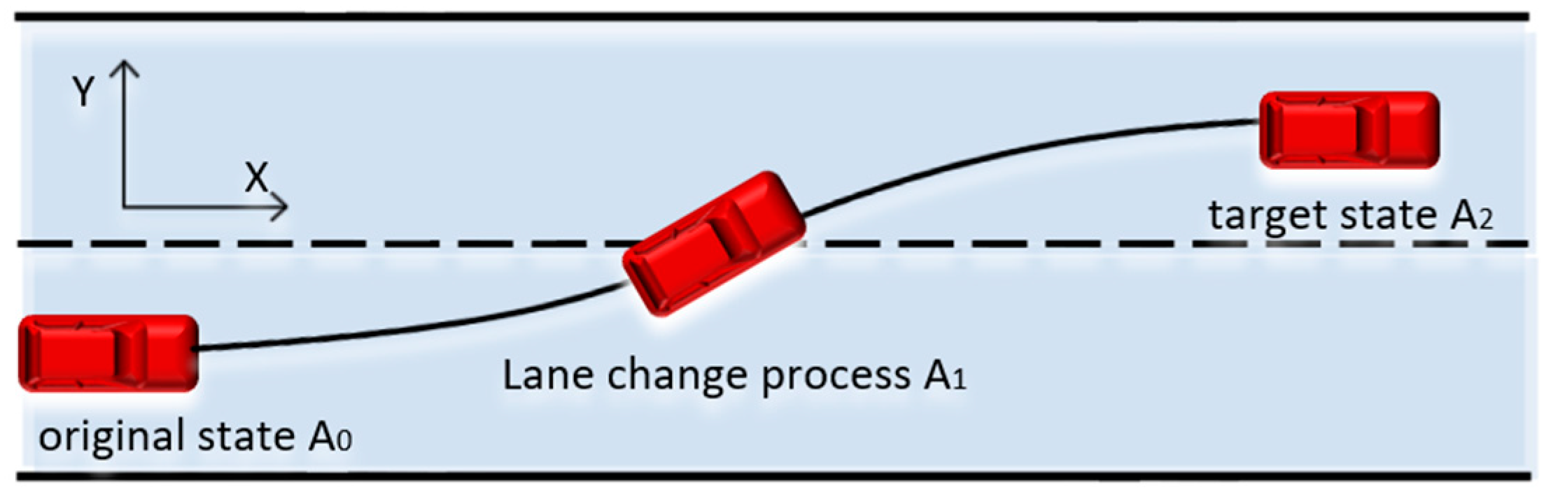
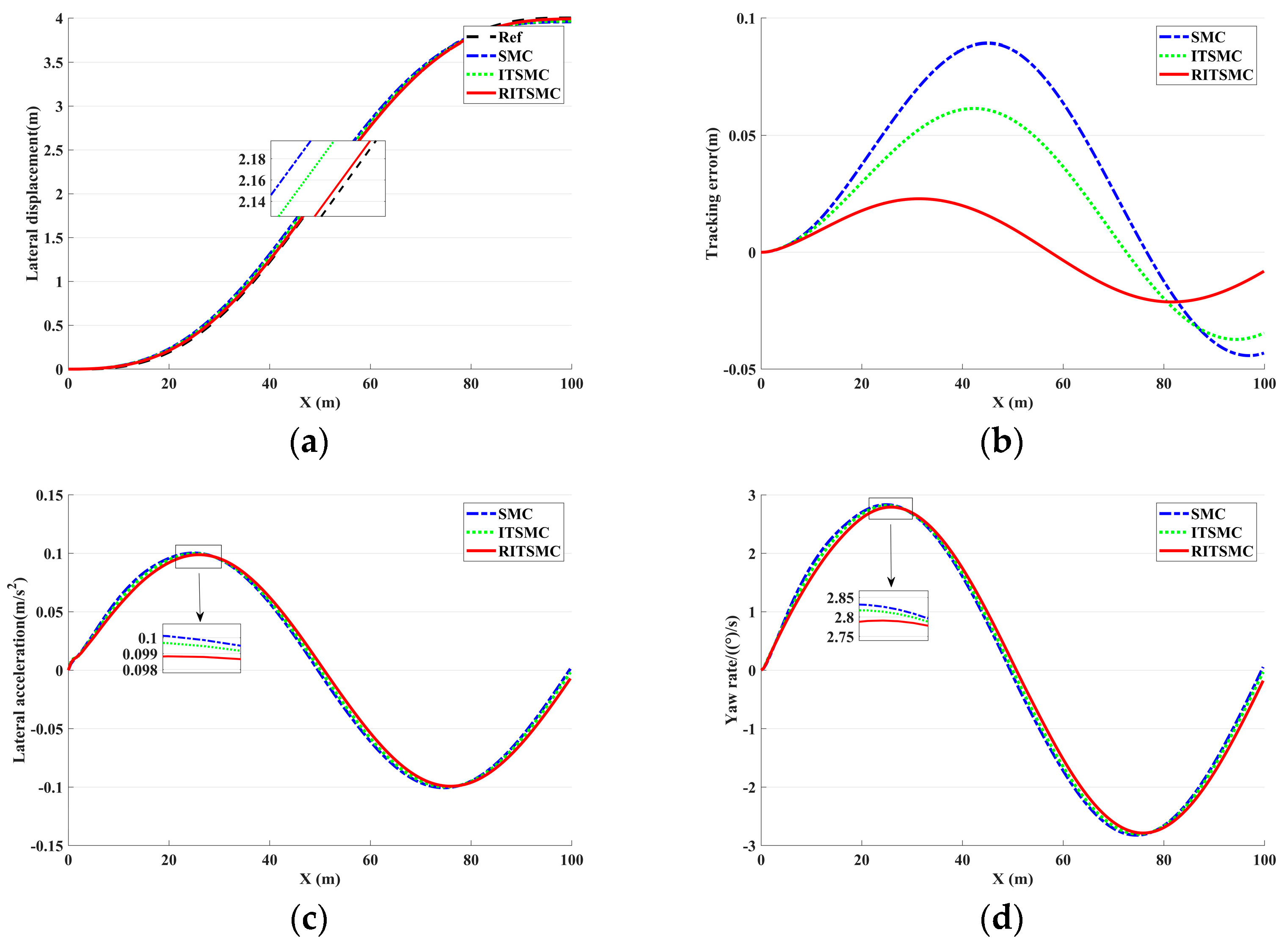
4.2. Single Lane Change: Comparison and Analysis of Controller Effects

In this section, we selected the lane-changing scenario as a case study to verify the effectiveness of the controller, as shown in Figure 7, and evaluated their performance in the lane-changing scenario through a comparative analysis of three different controllers. This further validates the stability of the designed controller under different road conditions, thereby improving the practical application ability of autonomous vehicles. To do so, we chose a lane-changing trajectory model as the reference signal for the system, which is:

$$\left\{\begin{array}{c}{Y}_r(x)=\frac{2}{\pi }(\pi +\frac{\pi }{50}(x-50)+sin(\frac{\pi }{50}(x-50)))\\ {\varphi }_r=\frac{2}{\pi }(\frac{\pi }{50}+\frac{\pi }{50}cos(\frac{\pi }{50}(x-50)))\end{array}\right.$$

(23)

where $Y_r$, $x$, ${\varphi }_r$ are the reference lateral position, reference longitudinal position, and reference yaw angle of the autonomous vehicle during its driving process, respectively.

4.2.1. Test Condition 1: Low-Speed Wet Slippery Road Surface

From Figure 8a, it can be seen that the three controllers generate different actual trajectories in the lane-changing scenario. The zoomed-in section of the figure reveals that the actual trajectories generated by the SMC and ITSMC controllers are the farthest from the reference trajectory (Ref), while the trajectory generated by the RITSMC controller is the closest to the reference trajectory. This indicates that the RITSMC controller exhibits precise trajectory tracking performance during lane-changing maneuvers. Additionally, by examining the simulation results in Figure 8b, it is evident that the RITSMC controller produces the smallest peak lateral error compared to the SMC and ITSMC controllers, demonstrating its superior trajectory tracking performance. Based on the data from

Table 5. Lane change peak error table.

Vehicle Speed/Road Grip /(km/h)	SMC/m	ITSMC/m	RITSMC/m	Opt1	Opt2
$0.45/54$	0.0795	0.059	0.022	72.3%	62.7%
$0.85/54$	0.078	0.058	0.02	74.4%	65.5%
$0.85/72$	0.09	0.061	0.028	68.9%	54%

, it is evident that RITSMC demonstrates a significant improvement in trajectory accuracy compared to SMC and ITSMC. This further proves the suitability of the proposed RITSMC controller not only for dual-lane scenarios but also for lane-changing scenarios, making it more aligned with the real-world driving requirements.

In Figure 8c, the results of three controllers controlling the vehicle’s lane changing on a wet road surface are shown. The results indicate that the maximum lateral acceleration peak generated during lane changing under the SMC controller is the highest, indicating that this controller has poor stability control over the vehicle during lane changing. Compared with the SMC controller, the ITSMC controller slightly reduces the lateral acceleration generated during lane changing, but it is clear from the graph that the RITSMC controller produces the smallest lateral acceleration peak during lane changing, indicating that this controller has far superior stability control over the vehicle compared to SMC and ITSMC. In Figure 8d, the maximum yaw rate peak generated during lane changing under the SMC controller is the highest, indicating that this controller makes it easy for the vehicle to lose stability during lane changing, thereby affecting the vehicle’s driving safety. In contrast, the ITSMC controller generates a slightly smaller yaw rate peak during lane changing, thus improving the vehicle’s driving stability. However, the RITSMC controller generates an even smaller yaw rate peak during lane changing, indicating that this controller can control the vehicle’s lane changing more stably. In Figure 8e shows the change in the vehicle’s lateral displacement during lane changing under the three different controllers. It is clear from the zoomed-in graph that the maximum lateral displacement peak generated during lane changing under the SMC controller is the highest, indicating that this controller is prone to causing severe fluctuations in vehicle driving and reducing its stability. However, compared to the SMC controller, the ITSMC controller generates a smaller lateral displacement peak during lane changing, indicating that it improves the vehicle’s driving stability to some extent. More importantly, the RITSMC controller generates the smallest lateral displacement peak during lane changing, which further indicates that this controller can control the vehicle’s turning more stably and improve its stability. In Figure 8f, the results of the three controllers’ control over the vehicle’s steering angle are shown. The zoomed-in graph clearly shows that on a wet road surface, the vehicle’s steering angle is smallest under the RITSMC controller and largest under the SMC controller, with the ITSMC controller generating a smaller steering angle than SMC but larger than RITSMC. This indicates that the vehicle’s turning under the RITSMC controller is more stable, can avoid sideslip, and thus improves the vehicle’s stability. Therefore, through simulation comparison and analysis of Figure 8e–f, we have verified that the proposed RITSMC control method in this paper can achieve dual advantages: precise trajectory tracking and optimal stability, greatly improving the safety and reliability of autonomous driving vehicles.

4.2.2. Test Condition 2: Low-Speed Dry Asphalt Pavement

By enlarging the trajectory tracking plots in Figure 9a, it can be observed that both SMC and ITSMC controllers exhibit the poorest fit between the actual and reference trajectories, indicating that these two controllers are not effective for keeping the vehicle on the desired path. Meanwhile, it can be clearly seen that the RITSMC controller generates the best fit between the actual and reference trajectories, indicating that this controller can better track the reference trajectory during lane changing maneuvers. Combining the lateral tracking errors in Figure 9b, we can compare the peak values of lateral errors generated by the three different controllers during vehicle lane changing. It can be found that SMC produces the largest error peak, ITSMC reduces the peak value compared to SMC, but from the enlarged plot, it is evident that the lateral error peak of RITSMC is the lowest, indicating that this controller can better control the vehicle’s trajectory tracking performance compared to the other two controllers. Based on the optimization results from Table 5, it is evident that RITSMC exhibits a significant improvement in trajectory tracking compared to SMC and ITSMC. Therefore, it can be concluded that using the RITSMC controller enables vehicles to travel more safely along the desired trajectory.

In Figure 9c, three controllers are shown controlling the lateral acceleration variation of the vehicle during lane changing. During the lane-changing process, the SMC controller produces the highest peak lateral acceleration, while the ITSMC controller produces a relatively smaller peak lateral acceleration compared to SMC, indicating that this controller improves the stability of the vehicle. However, as shown in the zoomed-in Figure 9c, the RITSMC controller produces the smallest peak lateral acceleration, indicating that the vehicle controlled by RITSMC is more stable and reliable than the vehicles controlled by SMC and ITSMC. In Figure 9d, due to the increase in the road adhesion coefficient, the lateral roll velocity amplitude of the vehicle is slightly reduced. Through the locally magnified graph, it is shown that the SMC-controlled vehicle produces the highest peak lateral roll velocity during lane changing, indicating that the vehicle is prone to shaking under SMC control, thereby reducing the stability of the vehicle. Although the ITSMC-controlled vehicle produces a smaller peak lateral roll velocity during lane changing, and the stability of the vehicle is improved, the RITSMC-controlled vehicle produces the smallest peak lateral roll velocity during lane changing, indicating that this controller provides the best stability for the vehicle. In Figure 9e, with the increase in the road friction coefficient, the fluctuation of the lateral deviation angle of the center of mass is slightly reduced. The SMC-controlled vehicle produces the highest peak lateral deviation angle and fluctuation during lane changing, indicating that this controller has the worst stability effect on the vehicle during lane changing. Although the ITSMC-controlled vehicle produces a smaller peak lateral deviation angle during lane changing, and the stability of the vehicle is further improved, the RITSMC-controlled vehicle produces the smallest peak lateral deviation angle and fluctuation during lane changing, indicating that this controller provides better stability for the vehicle during turning. In Figure 9f, comparing the three controllers, the SMC-controlled vehicle produces the largest peak front-wheel steering angle during lane changing, indicating that this controller produces the largest actual steering angle during the vehicle’s operation, and therefore the worst stability. In contrast, the RITSMC-controlled vehicle produces the smallest peak front-wheel steering angle during lane changing, and the ITSMC-controlled vehicle produces a peak front-wheel steering angle far greater than RITSMC, indicating that the RITSMC controller provides a more stable and reliable turning process. Therefore, in terms of vehicle control, the RITSMC controller performs the best, with higher stability and reliability, and can be used for actual vehicle control.

4.2.3. Test Condition 3: High-Speed Dry Asphalt Pavement

In Figure 10a, three controllers are shown controlling the vehicle’s output trajectory. As the speed increases, the tracking trajectories produced by the three controllers change significantly. The zoomed-in graph clearly shows that the SMC controller produces the greatest difference between the actual and reference trajectories when the vehicle changes lanes, indicating that this controller is not effective in tracking the reference trajectory. The ITSMC controller also produces a large difference between the actual and reference trajectories when the vehicle changes lanes. From the zoomed-in graph, it can be seen that only the RITSMC controller produces the best fit between the actual and reference trajectories when the vehicle changes lanes. Further combining the lateral error curve in Figure 10b, we can observe that the RITSMC controller generates the smallest peak lateral error, while the SMC and ITSMC controllers produce larger lateral errors compared to RITSMC. Based on the data from Table 5, it can be observed that RITSMC exhibits a significant improvement in trajectory tracking accuracy compared to SMC and ITSMC. Therefore, it can be conclusively stated that the RITSMC controller performs the best in tracking the reference trajectory.

In Figure 10c, as the speed of the controlled vehicle increases, the amplitude of its lateral acceleration also increases. The SMC-controlled vehicle produces the highest peak lateral acceleration during lane changing, indicating that this controller exhibits the poorest stability during lane changing. In contrast, the ITSMC-controlled vehicle generates a slightly smaller lateral acceleration peak than SMC, demonstrating some degree of stability improvement. However, the RITSMC-controlled vehicle produces a smaller lateral acceleration peak relative to ITSMC. This indicates that RITSMC can control the vehicle’s motion more stably than SMC and ITSMC during lane changing. In Figure 10d, as the speed of the controlled vehicle increases, the amplitude of the vehicle’s yaw rate increases. The zoomed-in section reveals that the SMC-controlled vehicle produces the largest peak yaw rate during lane changing is approximately $\pm 2.82((°)/\mathrm{s})$, indicating that the stability of the SMC-controlled vehicle during lane changing is the worst. The peak yaw rate change generated by ITSMC-controlled vehicle during lane changing is relatively smaller than that produced by SMC, and its stability is better than that of SMC. However, the peak yaw rate change produced by the RITSMC-controlled vehicle during lane changing is the smallest, measuring approximately ±2.79((°)/s). Therefore, controlling the vehicle to change lanes under this controller can be more stable and safe. In Figure 10e, as the vehicle speed increases, the fluctuation of the vehicle’s lateral displacement angle also increases. From the figure, it is evident that SMC-controlled vehicle produces the largest peak lateral displacement angle during lane changing, indicating that the stability of the SMC-controlled vehicle during turning is the worst. In comparison, the ITSMC-controlled vehicle produces a slightly smaller peak lateral displacement angle that SMC, indicating that this control has slightly improved the stability of the vehicle during turning. However, the peak lateral displacement angle produced by the RITSMC-controlled vehicle during lane changing is smaller than that produced by SMC and ITSMC. This indicates that RITSMC controls the turning of the vehicle more stably. In Figure 10f, as the vehicle speed increases, the magnitude of the tire angle also increases. From the zoomed-in section, it can be seen that the SMC-controlled vehicle produces the largest tire angle during lane changing, indicating that the SMC controller results in excessive tire angle during turning, which severely affects the stability. The ITSMC-controlled vehicle produces a smaller tire angle compared to SMC, indicating that this controller partially improves the stability of the vehicle during turning. However, the peak tire angle produced by the RITSMC-controlled vehicle during lane changing is much smaller than that produced by SMC and ITSMC. This indicates that RITSMC controls the turning of the vehicle with a minimum steering angle, thus maximizing the stability of the vehicle during turning. In summary, the simulation results fully illustrate that the RITSMC-controlled vehicle during lane changing has better stability and accurate trajectory tracking performance.

According to the data in Table 5, it can still be observed that the RITSMC control method maintains the minimum peak lateral error in lane change scenarios, indicating that the RITSMC achieves good trajectory tracking even in lane change situations. From the data in Figure 8c–f, Figure 9c–f and Figure 10c–f, although the output results of the three controllers are similar, it is evident that the RITSMC exhibits smaller fluctuations and peaks, indicating better stability. Taking into account the data from Table 4 and Table 5, it can be concluded that the RITSMC control method demonstrates wide applicability.

5. Conclusions

Due to the negative impact of external disturbances on autonomous vehicles, this article proposes a comprehensive RITSMC method that integrates recursive integral sliding mode surfaces, an exponential approaching law, and adaptive algorithms. The aim is to enhance the performance of autonomous vehicles and effectively address the issue of external disturbances.

(1) The study of disturbance terms is crucial for optimizing autonomous driving systems. Vehicles experience uncontrollable disturbances during actual operation, which affect trajectory tracking accuracy and driving stability. Considering these disturbance terms allows for the evaluation of control algorithm robustness and adaptability, leading to the adoption of superior control strategies to suppress the impact of disturbances.

(2) The adoption of the recursive integral sliding mode method can significantly improve the accuracy of autonomous driving systems, reduce oscillations, and enhance system robustness. By incorporating recursive integration, the system can better adapt to diverse driving environments, thereby tracking desired trajectories more stably and resisting external disturbances effectively.

(3) The exponential approaching law exhibits excellent stability and disturbance rejection performance, while featuring a simple algorithm structure and high computational efficiency. The adoption of the exponential approaching law method allows the system to converge to the desired state more rapidly and possess stronger capabilities to suppress external disturbances.

(4) The adaptive algorithm enhances the adaptability and response speed of the control system to external disturbances by dynamically adjusting the control parameters on the sliding mode surface. This enables the trajectory tracking error to converge to zero more quickly, thereby achieving optimal closed-loop tracking performance and stability.

By comparing the simulation results under various operating conditions and road segments, it was observed that the proposed RITSMC controller can effectively control the vehicle to travel on the desired trajectory with high precision and strong stability even in the presence of external disturbances. In contrast, the SMC and ITSMC controllers fail to effectively track the desired trajectory and improve stability when subjected to disturbances. Therefore, it can be concluded that RITSMC addresses the issue of external disturbance impact on vehicle trajectory tracking in a superior manner in practical applications.

However, this study also has some limitations. As it was conducted in a simulation environment, despite incorporating diverse driving scenarios, the complexity and variability of real-world road environments still pose a challenge. Therefore, future research needs to be carried out in two aspects: (1) Applying the algorithm to actual vehicles and considering the impact of more real-world scenarios and environmental factors on the algorithm. (2) Exploring the integration of this algorithm with other control algorithms to further enhance the tracking accuracy and stability of autonomous vehicles.

References

1. Dong, L.; Sun, D.; Han, G.; Li, X.; Hu, Q.; Shu, L. Velocity-Free Localization of Autonomous Driverless Vehicles in Underground Intelligent Mines. IEEE Trans. Veh. Technol. 2020, 69, 9292–9303. [Google Scholar] [CrossRef]
2. Li, Y.; Feng, H.; Peng, Z.; Zhou, L.; Wan, J. Diversity-aware unmanned vehicle team arrangement in mobile crowdsourcing. EURASIP J. Wirel. Commun. Netw. 2022, 2022, 56. [Google Scholar] [CrossRef]
3. Karmakar, G.; Chowdhury, A.; Das, R.; Kamruzzaman, J.; Islam, S. Assessing Trust Level of a Driverless Car Using Deep Learning. IEEE Trans. Intell. Transp. Syst. 2021, 22, 4457–4466. [Google Scholar] [CrossRef]
4. Dong, H.; Xi, J. Model Predictive Longitudinal Motion Control for the Unmanned Ground Vehicle with a Trajectory Tracking Model. IEEE Trans. Veh. Technol. 2021, 71, 1397–1410. [Google Scholar] [CrossRef]
5. Song, X.; Shao, Y.; Qu, Z. A Vehicle Trajectory Tracking Method with a Time-Varying Model Based on the Model Predictive Control. IEEE Access 2019, 8, 16573–16583. [Google Scholar] [CrossRef]
6. Lu, S. Path Tracking Control Algorithm for Unmanned Vehicles based on Improved RRT Algorithm. In Proceedings of the IEEE 2nd International Conference on Electronic Technology, Communication and Information (ICETCI’22), Changchun, China, 27–29 May 2022; pp. 1201–1204. [Google Scholar]
7. Yang, C.; Liu, J. Trajectory Tracking Control of Intelligent Driving Vehicles Based on MPC and Fuzzy PID. Math. Probl. Eng. 2023, 2023, 2464254. [Google Scholar] [CrossRef]
8. Liu, M.; Zhao, F.; Yin, J.; Niu, J.; Liu, Y. Reinforcement-Tracking: An Effective Trajectory Tracking and Navigation Method for Autonomous Urban Driving. IEEE Trans. Intell. Transp. Syst. 2021, 23, 6991–7007. [Google Scholar] [CrossRef]
9. Zuo, Z.; Yang, X.; Li, Z.; Wang, Y.; Han, Q.; Wang, L.; Luo, X. MPC-Based Cooperative Control Strategy of Path Planning and Trajectory Tracking for Intelligent Vehicles. IEEE Trans. Intell. Veh. 2020, 6, 513–522. [Google Scholar] [CrossRef]
10. Nie, Y.; Hua, Y.; Zhang, M.; Zhang, X. Intelligent Vehicle Trajectory Tracking Control Based on VFF-RLS Road Friction Coefficient Estimation. Electron 2022, 11, 3119. [Google Scholar] [CrossRef]
11. Huang, C.; Huang, H.; Zhang, J.; Hang, P.; Hu, Z.; Lv, C. Human-Machine Cooperative Trajectory Planning and Tracking for Safe Automated Driving. IEEE Trans. Intell. Transp. Syst. 2021, 23, 12050–12063. [Google Scholar] [CrossRef]
12. Nie, Y.; Zhang, M.; Zhang, X. Trajectory Tracking Control of Intelligent Electric Vehicles Based on the Adaptive Spiral Sliding Mode. Appl. Sci. 2021, 11, 11739. [Google Scholar] [CrossRef]
13. Wang, H.; Liu, B. Path Planning and Path Tracking for Collision Avoidance of Autonomous Ground Vehicles. IEEE Syst. J. 2021, 16, 3658–3667. [Google Scholar] [CrossRef]
14. Huang, Y.; Chen, Y. Vehicle Lateral Stability Control Based on Shiftable Stability Regions and Dynamic Margins. IEEE Trans. Veh. Technol. 2020, 69, 14727–14738. [Google Scholar] [CrossRef]
15. Cheng, S.; Li, L.; Guo, H.Q.; Chen, Z.G.; Song, P. Longitudinal Collision Avoidance and Lateral Stability Adaptive Control System Based on MPC of Autonomous Vehicles. IEEE Trans. Intell. Transp. Syst. 2019, 21, 2376–2385. [Google Scholar] [CrossRef]
16. He, X.; Liu, Y.; Lv, C.; Ji, X.; Liu, Y. Emergency steering control of autonomous vehicle for collision avoidance and stabilisation. Veh. Syst. Dyn. 2019, 57, 1163–1187. [Google Scholar] [CrossRef]
17. Zhang, Z.; Guo, Y.; Gong, D.; Liu, J. Global Integral Sliding-Mode Control with Improved Nonlinear Extended State Observer for Rotary Tracking of a Hydraulic Roofbolter. IEEE ASME Trans. Mechatron. 2022, 28, 483–494. [Google Scholar] [CrossRef]
18. Liu, Y.; Yuan, L.; Chen, H.; Wang, P.; Xu, A. Design of single neuron super-twisting sliding mode controller for permanent magnet synchronous servo motor. Front. Energy Res. 2023, 11, 34. [Google Scholar]
19. Truong, T.N.; Vo, A.T.; Kang, H.J. A Backstepping Global Fast Terminal Sliding Mode Control for Trajectory Tracking Control of Industrial Robotic Manipulators. IEEE Access 2021, 9, 31921–31931. [Google Scholar] [CrossRef]
20. Liu, Y.; Yan, W.; Zhang, T.; Yu, C.; Tu, H. Trajectory Tracking for a Dual-Arm Free-Floating Space Robot with a Class of General Nonsingular Predefined-Time Terminal Sliding Mode. IEEE Trans. Syst. Man Cybern. Syst. 2021, 52, 3273–3286. [Google Scholar] [CrossRef]
21. Hu, Y.; Wang, H.; He, S.; Zheng, J.; Ping, Z.; Shao, K.; Cao, Z.; Man, Z. Adaptive Tracking Control of an Electronic Throttle Valve Based on Recursive Terminal Sliding Mode. IEEE Trans. Veh. Technol. 2020, 70, 251–262. [Google Scholar] [CrossRef]
22. Mofid, O.; Mobayen, S. Adaptive sliding mode control for finite-time stability of quad-rotor UAVs with parametric uncertainties. ISA Trans. 2018, 72, 1–14. [Google Scholar] [CrossRef] [PubMed]
23. Ghadiri, H.; Montazeri, A. Adaptive Integral Terminal Sliding Mode Control for the Nonlinear Active Vehicle Suspension System under External Disturbances and Uncertainties. IFAC PapersOnLine 2022, 55, 2665–2670. [Google Scholar] [CrossRef]
24. Bei, S.; Hu, H.; Li, B.; Tian, J.; Tang, H.; Quan, Z.; Zhu, Y. Research on the Trajectory Tracking of Adaptive Second-Order Sliding Mode Control Based on Super-Twisting. World Electr. Veh. J. 2022, 13, 141. [Google Scholar] [CrossRef]
25. Ji, X.; He, X.; Lv, C.; Liu, Y.; Wu, J. Adaptive-neural-network-based robust lateral motion control for autonomous vehicle at driving limits. Control Eng. Pract. 2018, 76, 41–53. [Google Scholar] [CrossRef]
Figure 1. Schematic diagrams of vehicle dynamics model and vehicle kinematics model.
Electronics 12 02748 g001
Figure 2. Architecture block diagram of lateral motion controller.
Electronics 12 02748 g002
Figure 3. Simulated driving track of double line shifting.
Electronics 12 02748 g003
Figure 4. Results of double lane change on a low-speed wet road surface. (a) Lateral displacement of the vehicle; (b) lateral error of the vehicle; (c) lateral acceleration of the vehicle; (d) yaw rate of the vehicle; (e) lateral tilt angle of the vehicle’s center of gravity; (f) steering angle of the vehicle’s front wheels.
Electronics 12 02748 g004aElectronics 12 02748 g004b
Figure 5. Results of double lane change on a low-speed dry asphalt road surface. (a) Lateral displacement of the vehicle; (b) lateral error of the vehicle; (c) lateral acceleration of the vehicle; (d) yaw rate of the vehicle; (e) lateral tilt angle of the vehicle’s center of gravity; (f) steering angle of the vehicle’s front wheels.
Electronics 12 02748 g005
Figure 6. Results of double lane change on a high-speed dry asphalt road surface. (a) Lateral displacement of the vehicle; (b) lateral error of the vehicle; (c) lateral acceleration of the vehicle; (d) yaw rate of the vehicle; (e) lateral tilt angle of the vehicle’s center of gravity; (f) steering angle of the vehicle’s front wheels.
Electronics 12 02748 g006aElectronics 12 02748 g006b
Figure 7. Simulation of autonomous vehicle lane change trajectory.
Electronics 12 02748 g007
Figure 8. Results of lane changing on a low-speed wet road surface. (a) Lateral displacement of the vehicle; (b) lateral error of the vehicle; (c) lateral acceleration of the vehicle; (d) yaw rate of the vehicle; (e) lateral tilt angle of the vehicle’s center of gravity; (f) steering angle of the vehicle’s front wheels.
Electronics 12 02748 g008
Figure 9. Results of lane change on a low-speed dry asphalt road surface. (a) Lateral displacement of the vehicle; (b) lateral error of the vehicle; (c) lateral acceleration of the vehicle; (d) yaw rate of the vehicle; (e) lateral tilt angle of the vehicle’s center of gravity; (f) steering angle of the vehicle’s front wheels.
Electronics 12 02748 g009
Figure 10. Results of lane changing on a high-speed dry asphalt road surface. (a) Lateral displacement of the vehicle; (b) lateral error of the vehicle; (c) lateral acceleration of the vehicle; (d) yaw rate of the vehicle; (e) lateral tilt angle of the vehicle’s center of gravity; (f) steering angle of the vehicle’s front wheels.
Electronics 12 02748 g010aElectronics 12 02748 g010b