Design and Implementation of a Hierarchical Digital Twin for Power Systems Using Real-Time Simulation

Abstract

This paper presents a hierarchical Digital Twin architecture and implementation that uses real-time simulation to emulate the physical grid and support grid planning and operation. With the demand for detailed grid information for automated grid operations and the ongoing transformation of energy systems, the Digital Twin can extend data acquisition by establishing a reliable real-time simulation. The system uses observer algorithms to process model information about the voltage dependencies of grid nodes, providing information about the dynamic behavior of the grid. The architecture implements multiple layers of data monitoring, processing, and simulation to create node-specific Digital Twins that are integrated into a real-time Hardware-in-the-Loop setup. The paper includes a simulation study that validates the accuracy of the Digital Twin, in terms of steady-state conditions, dynamic behavior, and required processing time. The results show that the proposed architecture can replicate the physical grid with high accuracy and corresponding dynamic behavior.

1. Introduction

1.1. Motivation

The ongoing transformation of the electrical power system towards renewable energies and more decentralized structures is driven by climate change and political decisions. This structural change in power generation is accompanied by the increasing digitalization and automation of the grids. Previously centralized systems with high system inertia are becoming decentralized and replaced by converter-driven systems with high dynamics and many variables influencing the system behavior. In addition, the system operation and grid stabilization focus more and more on distribution grids that integrate a significant amount of renewable energy. The structural change in electricity generation requires a change in the system operation. Key drivers from the field of Industry 4.0 are being transferred and applied to enable the energy transition with digitalization, automation, and modern information and communication technology [1].

The focus is especially on the distribution grids, namely the medium and low-voltage level. Compared with high-voltage transmission grids, these have a significantly lower level of automation. As part of the structural change, intelligent solutions are increasingly being installed and integrated into the control system. The widespread use of IP-based protocols, like IEC 61850 [2] and IEC 60870-5-104 [3], improves the observability of the grid and its state by providing more information about the system. Digital substations that rely on fully IP-based communication offer advantages in terms of system integration, system operation, and IT security [4]. In addition to the process-related advantages, digitalized processes enable investigations and analyses that generate additional values in operation that go beyond classic monitoring [5]. Furthermore, transformer stations in low voltage grids are increasingly equipped with integrated measurement devices and provide data for local grid management and for the overlaying control and monitoring processes. Digitized grids thus improve grid transparency by providing measured data for grid operation tasks via communication interfaces. A more detailed and accurate monitoring of the grid state provides the basis for an automated grid operation management of distribution grids.

Due to the change in system dynamics caused by new feed-in and load behavior, distribution system operators will increasingly have to take control of the system. In addition, power overloads and voltage stability problems caused by local power gradients of electric vehicles and heat pump systems will have to be controlled. The large number of controllable plants requires a transition to automated grid management processes [6].

The system’s observability is the crucial factor for the feasibility of all the processes, such as re-powering after failure, switching operations, or performing preventive and curative congestion management. In addition to the actual measurements, which are widely distributed throughout the grid, this also includes the status of the lines and the positions of the switches in meshed or partially meshed grid sections. In the future, a wide variety of heterogeneous data sources will interact with each other and increase the observability of the system [7]. Micro-sensors, intelligent measuring systems, or phasor measurement units can record the status over a wide range of the grid. In addition to knowledge about the grid state, it is also essential to increase the modeling ability of the system. This means grid models that represent the current state are necessary and can be used as test platforms. This includes local monitoring in the form of dynamic observations of different grid and system configurations, as they are used as concepts for DSA tools in the transmission network area [8]. Different test platforms are becoming widely developed to cope with the different challenges posed by the increasing complexities. Real-time (RT) simulation and closed-loop applications are mostly part of the test benches, as they provide the opportunity to connect digital, as well as physical, assets. The focus of the applications varies between plant-specific test beds for wind turbines [9] up to detailed grid simulations [10,11]. Besides the differences in the design and integration of digital and physical assets, the focus is on replicating real-world behavior and providing a platform for development and validation.

The challenges in reproducing the actual grid state lie in processing the recorded data and the comparison with the simulation models. Measured data does not provide any information about the connected systems and can only be used to assess the current state. Essential system parameters of the connected loads and feeds can only be considered via generalized assumptions. But the system behavior of the assets is an essential part of the investigations to enable a correct estimation of automated interventions. The correct mapping therefore requires a high degree of knowledge about the systems connected to the grid.

1.2. Digital Twin Overview and Applications

New grid operation supporting technologies are being developed and deployed within electrical energy systems. Due to the demands of grid state observability in highly automated grids, the concept of Digital Twins (DT) has been adopted into energy systems to increase grid monitoring capabilities [12]. Originally from the industrial sector, DTs describe a virtual representation of a physical system, asset and/or process. Replicating the real systems includes software, hardware, and data integration to provide RT monitoring, controlling, prediction, optimization, and improved decision-making [13,14]. The concept of the DT describes a setup of components to observe a system’s physical behavior and transfer it into a digital replication. The key components include the measurement of the real system, the virtual/digital model of the system, the data transmission between the real and simulated system, and the provided services [15]. An integral aspect of a DT is the online coupling with the physical system, such that the system parameters are continuously adapted and can provide additional information.

The applications in the field of research and development of DTs in electrical power systems include individual components, grid areas, control center applications, and protection technology [16,17,18,19]. In [20], a modular framework for implementing a power system DT for operation and planning is proposed. The concept in [21] describes a detailed DT for transformers to estimate the primary measurement values based on the secondary side measurements. In [22], DTs are used for virtual testing of protection systems, enabling verification of the design and performance of individual assets and entire protection systems. The approach also provides cost-effective training opportunities and presents the testing and results of a line distance protection relay using virtual and physical twins of the protection relay. The approach in [23] introduces an anomaly detection model based on DTs for utility gas turbines. Regarding SCADA assistant functionalities, [24] implements DTs to assess contingency mitigation strategies and to support decision-making processes under different system conditions.

1.3. Concept of Hierarchical Digital Twins to Improve Simulation Quality

As described earlier, the observability of the grid forms the essential basis for future developments in distribution grids. Through the provision of essential grid and measurement data as well as computable grid models, planning and operation tasks can be supported. The approach of a hierarchical DT offers the possibility to provide the latest system parameters as an online coupled application.

The developed hierarchical DT comprises multiple components, which together enable the emulation of the actual grid status within a RT simulation. The structure is divided into different subsections related to data acquisition, processing, and simulation. The real-time interface (RTI) is a computing module that processes the measurement data and calculates node-specific DTs containing model and power quality information. As the simulation part, a RT simulation is coupled with the RTI via a Hardware-in-the-Loop (HiL) configuration. This integrates the node-specific DTs into a higher-level grid simulation and enables data exchange between the model and the simulation. The result is a RT simulation that can be influenced and, due to the hierarchically integrated DTs, represents the grid that is constantly aligned with the real process.

The resulting system provides a more detailed and dynamic representation of the system state compared to traditional state estimation and monitoring systems. In contrast to these applications, the hierarchical DT includes information about the actual state as well as the dynamic behavior of each grid node. Based on models for each node, observers adapt the parameters for loads and feed-ins online during the operation of the grid. In a first implementation, the model focuses on changes in the voltage dependence of the active and reactive power caused by variations in the connected load and the feed-in situation. Due to the RT simulation, this approach enables the creation of digital snapshots of the physical grid and can be used for automated testing of switching, optimization, parameterization, and validation of grid operations. A major property of the approach is the flexible integration of vendor-agnostic RT simulation systems. The proposed hierarchical DT processes all information and provides the node behavior of the grid to a simulation platform. The RT simulation used is a fitting tool to realize the DT of the physical grid, but it can also be replaced by other systems. The focus of the investigation determines which simulation system should be used.

Accordingly, the main contributions of the work consist of the following aspects:

• Extension of measurement data regarding dynamic behavior;
• Continuous online adaption of model parameters with observer algorithms;
• Hardware-in-the-Loop coupled with real-time simulation to provide an online emulation of the physical system;
• Digital snapshots of grid situations for commissioning and operation;
• Vendor-agnostic real-time simulation system for Digital Twin setup.

The following article describes the setup and application of the hierarchical DTs detailed in Section 2. Especially the RT interface is in focus, as it contains essential data processing and distribution functions. Section 3 highlights data communication as one key function of the entire process. In addition, the observer algorithm and HiL setup are shown in this section. The laboratory setup for the development, testing, and validation of the processes is described in Section 4. Finally, Section 5 presents the DT results, including graphs of the transfer of steady-state conditions and dynamic behavior to the DT. It also provides an evaluation of the transfer and computation time for the entire process.

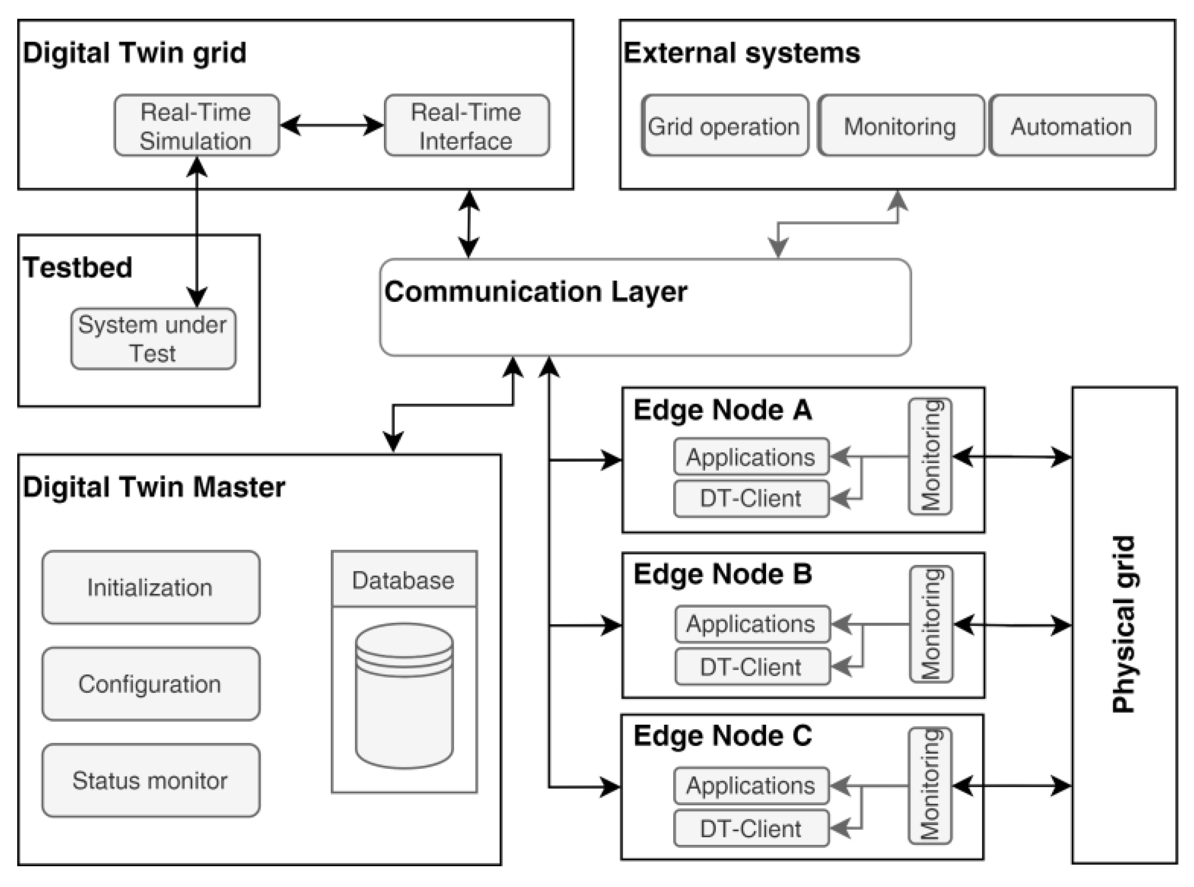
2. Setup and Applications of Hierarchical Digital Twins

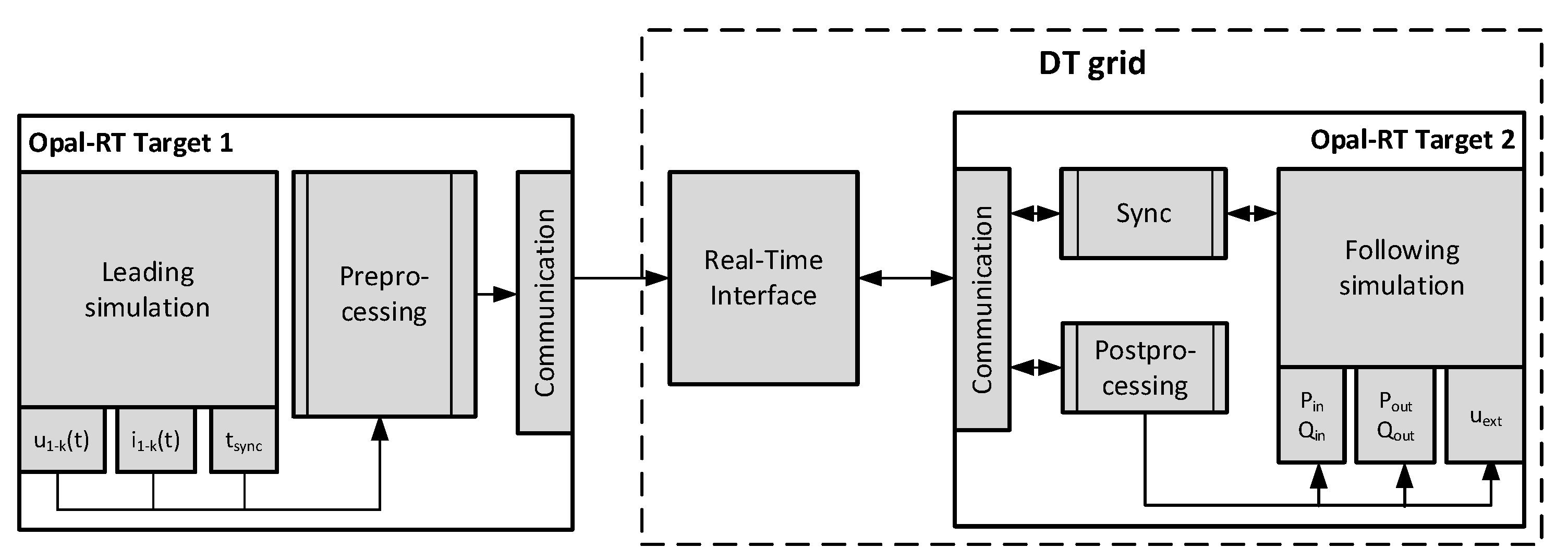
2.1. System Setup and Communication Links

SCADA systems are complex applications with various functionalities for the monitoring, operating, and assisting of electrical grids [25]. The state estimation function is crucial for monitoring applications as it computes all system state variables from measurements and topology information [26]. However, common state estimation algorithms run as steady-state calculations, which cannot provide a detailed representation of the system dynamics. Although state estimation is a useful tool for monitoring and planning tasks, it is still impractical for the online testing of system operations, since it relies on measurements, and no information on future dynamic behavior is available.

Operating decentralized grid automation requires more advanced system monitoring and estimation functionalities. Future automation functions, such as congestion management, voltage regulation, and operation, require more detailed information to process their optimal operations [27,28]. To address these challenges, the hierarchical DT approach combines algorithms for state estimation, power quality monitoring, and observer-based node modeling with RT simulation in a digital representation of the physical grid. This digital representation emulates the system state using the processed grid measurements and topology information, providing a tunable simulation.

The approach involves various levels of data aggregation and processing to establish the DT of the grid. Figure 1 shows the entire system setup, including the system links.

The system is connected to monitoring systems that provide the data from the physical grid. This monitoring setup is integrated into edge nodes that handle the first step of data processing and distribution. The local high-resolution data is used to compute power quality information and observer algorithms within a DT-Client application. This application forms the basis for the central DT application to align the RT simulation to the physical grid state. Due to the setup, additional applications can be integrated into the edge nodes to monitor or control the network.

As a supporting functionality of the setup, a DT Master is implemented to control the DTs of the edge nodes. These node DT-Clients are independent systems that can reflect the system behavior, but they need basic information to adapt their monitoring applications and variables. The DT Master provides this information and enables the initialization and configuration. Because of its centralized functionality for controlling the edge nodes, the DT Master also monitors the status information of the edge nodes.

A communication layer with connections to all major parts of the system handles the interaction between all components. The implementation of the edge nodes and the central communication interfaces are designed to handle different types of data and protocols. The architecture of such structures must be scalable for many observed grids and flexible enough to integrate different types of systems. Because of the paper’s focus on the modeling perspective, the communication layer is not described in detail. Referring to [29], a broker cluster architecture is proposed to integrate all systems into a flexible architecture. External systems can be connected to the communication interfaces to provide additional data or get information from the different applications and DTs.

The DT grid combines the field data from the edge nodes with grid topology and status information to establish a RT simulation aligned to the physical grid. The DT grid is divided into the two main processes of RTI and RT simulation. The RTI is the central platform for data processing into node-specific DTs as the underlying step of the hierarchical structure of the DT grid. Connected via a Hardware-in-the-Loop setup to the RT simulation, the node-specific DTs provide dynamic load and feed-in information for each grid node. The resulting grid DT corresponds to the actual state of the physical grid to provide a monitoring and simulation platform for further investigation. A connected test bed enables the interaction of physical or virtual applications with the DT grid.

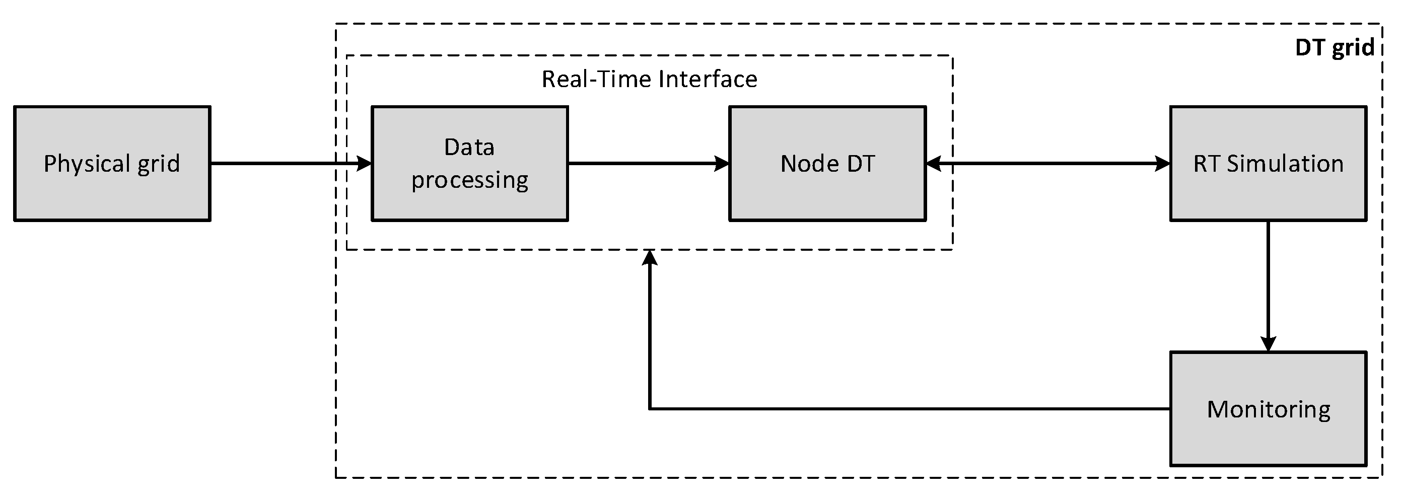
2.2. Real-Time Interface and HiL-Coupled Real-Time Simulation

The RTI is a toolchain to create node-specific DTs for integration into the RT simulation. The node DTs contain information about load and feed-in characteristics as well as the dynamic behavior regarding the voltage dependence of the active and reactive power. The RT simulation uses this information to process the grid simulation and provide grid information about grid status such as voltage levels or line load. Using Hypersim from Opal-RT, the RTI enables accurate and reliable simulations of electrical power grids, making it a valuable tool for research and development.

RT simulation is becoming an increasingly common tool for the research and development of electrical power grids across a wide range of topics [30,31]. The scope of the RT simulation can vary depending on the type of simulation being performed. For example, the time step can range from microseconds in EMT simulation to milliseconds in RMS simulation. Regardless of the time step used, it is important that the step size remains consistent for each iteration of the simulation. One of the major advantages of RT simulation is its ability of Hardware-in-the-Loop (HiL) or Controller-in-the-Loop (CiL), which allows for interaction between the simulation and external processes or devices. This provides a valuable tool to test and analyze the behavior of electrical power systems and to identify potential issues or areas for improvement. The RTI uses a HiL setup to integrate the node DTs into the DT grid. Figure 2 illustrates that principal HiL setup of the components to build the DT grid.

The inputs and outputs of the RTI are connected to the RT simulation, which contains the grid model of the physical grid. Based on the input of load and feed-in information from node DTs, the simulation processes the grid responses and loops back the measured signals. While respecting the RT condition, the node DTs can be included in the simulation and react according to the grid state. In this configuration, the system responds to external triggers or events as a preconfigured simulation. Via the monitoring connection, the results of the RT simulation are fed back into the RTI to compare and validate the simulation with the physical grid. The continuous process enables a constant emulation of the actual grid state.

In addition to the grid model itself, the accuracy of the DT grid depends on the quality of modeling and accuracy as input of the simulation. Since all load and feed-in information relies on the node DTs, the main process of the RTI is to model and compute the monitoring data. The calculation of the final node DTs is divided into monitoring and calculation functions and as a result is processed into a constant data stream of active and reactive power information for each grid node. The full data processing and provisioning process of the RTI is shown in Figure 3.

Nearly all nodes of interest in the considered MV grid are assumed to be monitored with voltage, current, and power flow information. The edge nodes can provide and transmit the required information to the RTI.

The monitoring process of the RTI system describes the data analysis of the actual measured grid state. Information about power quality phenomena is condensed into characteristics such as voltage harmonics or flicker. This node-specific information is used to validate the resulting RT simulation by comparing the simulation results. The information is also used to integrate the behavior of the node with characteristics not yet considered in the dynamic model, such as actual measured harmonics. In addition to power quality analysis, a state estimation is continuously performed to estimate missing node data due to missing metering devices or communication errors. The state estimation can also be used to detect bad data or errors in the grid model database to improve the DT grid database.

The calculation function is the second main part for processing the received data into information about the grid and performing system identification for each node. Based on information from the state estimation and monitoring systems, each node is analyzed for status and basic information, such as standard power consumption or feed-in. Available asset information about the type and characteristics of the connected system is also implemented into the node model. These inputs result in an initial setpoint for the observer, which is performed in the last step of this module. To obtain the dynamic behavior of the network node in terms of voltage dependencies, each node is sampled independently. During online operation, the observer obtains the deviation between the output model and the measured signal to continuously process the parameterization of the model. As one of the central applications, detailed information about the implementation and modeling is provided in Section 3.2.

As a result of the monitoring and calculation processes, every grid node is characterized by a dynamic model as well as information about harmonics and power quality properties. In addition to the characteristics, it is important to consider time references for the parameter sets. Especially when transmitted into RT simulation, the time base of the characteristics must be synchronized to each other to guarantee the validity of the simulation. The central database collects all information and forwards it to the HiL interface for RT simulation (see Section 3.1). Node-specific DTs are the aggregation of all gathered information and generate a constant value stream of load and feed-in equivalents for the simulation. The HiL requires secondary functions for validation and synchronization of all nodes to the same time base in addition to the value stream. Furthermore, the HiL coupling must be done with a fitting interface algorithm to avoid oscillations in the system. More information about the HiL setup and interfacing algorithms is described in Section 3.3. The grid basis of the RT simulation itself is configured as equal to the database information. Detected topology events are continuously updated to ensure that the grid state always matches the physical grid. The resulting DT of the distribution grid contains finally the process functions of RTI and the HiL-coupled RT simulation. Due to the hierarchical approach, the simulation platform of the DT grid is interchangeable as its main function is to simulate the pre-processed node and grid information. All grid state information and RT simulation results are available for external use via the database and flexible communication interfaces. Based on internal TCP/UDP communication, the access via standardized protocols such as IEC 61850 [2] or IEC 60870-5-104 [3] can be easily extended.

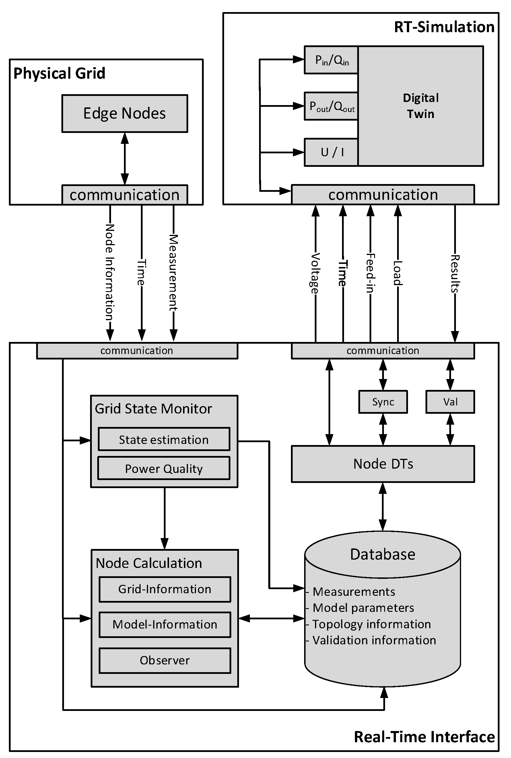
3. Implementation of Key Components of the Real-Time Interface

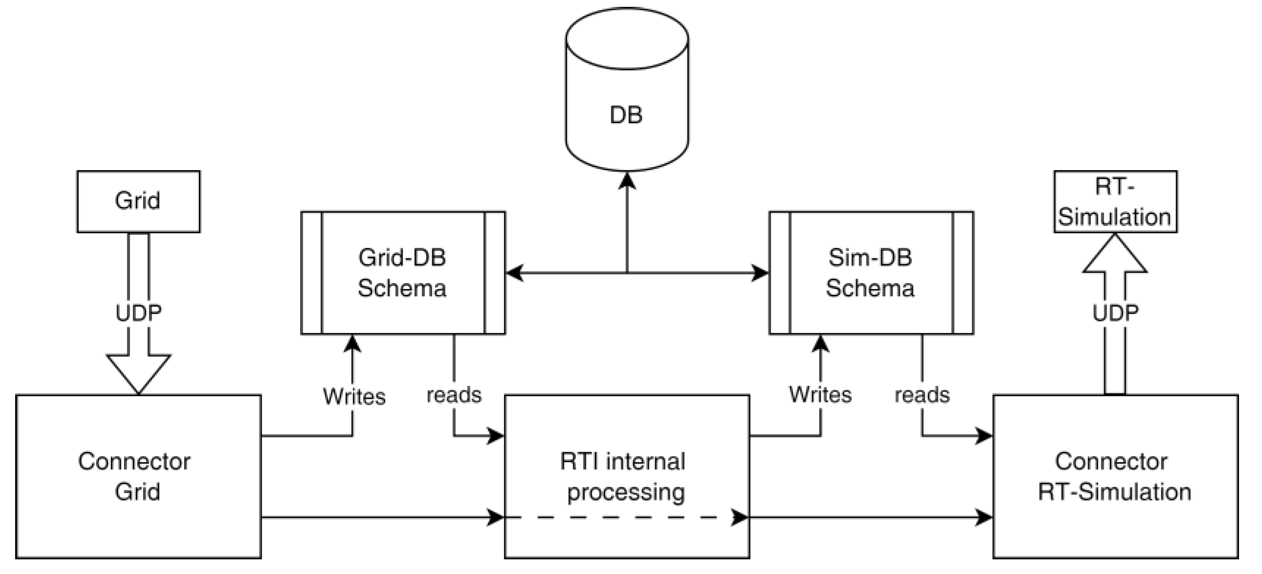
3.1. Communication and Signal Exchange

The UDP network protocol is used to connect the RT interface with the simulation environments. The UDP, or User Datagram Protocol, is a simple and efficient communication protocol that allows devices to send and receive data over a network. One of the UDP’s main advantages is its speed. Because it does not require the overhead of establishing and maintaining a connection, it can transmit data much faster than other protocols such as the TCP.

The UDP transfers data quickly and efficiently between the RT interface and the RT simulation, enabling a more accurate and responsive DT. Another advantage of the UDP is its simplicity. It has a small header and does not require complex handshaking or error checking, making it easy to implement and use. This makes it a suitable solution for prototype application where simplicity and the ability to adapt quickly is important.

In the context of a DT for grid monitoring and simulation, the delays introduced by the UDP will depend on several factors, including the distance between the transmitter and receiver, the speed of the network, and the load on the network. But in general, the UDP is known for having low latency compared to other protocols such as the TCP, because it does not have the overhead of establishing and maintaining a connection and does not perform error checking or retransmitting lost packets. However, this also means that the UDP is less reliable than the TCP, as it does not guarantee that all packets will be received. The impact of this on a DT will depend on the specific requirements of the application, but for the current state, the lower transmission delay is preferred for implementation. However, if reliability is more important at a later stage of development, then the common TCP-based energy protocols may be an appropriate choice as they can ensure that all packets are received [32]. It is also worth noting that the delays introduced by the UDP can be minimized by optimizing the network and the devices transmitting and receiving the data. In addition, implementing strategies such as packet aggregation and compression can also help reduce delays and improve the efficiency of the transmission.

The communication of the RT interface is divided into two signal paths. The first and fast pass directly through processes of the incoming UDP stream via node calculation and grid state monitoring (see Figure 3). This direct data stream is used for time-critical signals, which must process with the lowest possible time delay, like fast voltage events or faults. The usual data path depends on a central database to store and manage the datasets. The structure of the database connections is shown in Figure 4.

The database is designed with two schemas to support efficient data processing. The first schema is responsible for writing incoming field data into the database and retrieving values for the RTI internal processing components. The second schema is responsible for writing the processing results to the database and providing them to the RT simulation. The first schema plays a critical role in data acquisition, allowing the system to collect and store incoming field data in real time. This schema is optimized for fast write speeds to ensure that data is captured and stored efficiently. It is also designed to read data quickly and efficiently for use in RTI’s internal processing components. The second schema is responsible for writing the results of the RTI internal processing components back to the database. These results are then available for use in the RT simulation. This schema ensures that the processing results are easily accessible to the RT simulation. Overall, the two schemas work together to ensure that data is captured, processed, and made available for use in the RT simulation most efficiently.

3.2. Observer-Based Modeling of Grid Nodes

One of the central applications of the system is the ability to emulate the dynamic behavior of the physical grid within the RT simulation. To achieve this, the node DTs model the voltage and frequency-dependent load behavior of the grid nodes. With the increasing use of power-electronic components, the behavior of the system becomes more complex and cannot be described by traditional ohmic-inductive load characteristics. Therefore, it is important to accurately calculate the grid nodes’ voltage and frequency dependencies to reflect the system’s actual behavior. To accomplish this, each node of the medium voltage grid in the RT simulation is coupled to a model-based node DT. The node DTs are designed to reflect the voltage dependencies of the summarized loads for the underlying low-voltage grid. By modeling the behavior of the grid nodes in this way, the system can accurately reflect the dynamic behavior of the physical grid in RT simulation.

The type and parameterization of the modeling is a key factor in power system analysis [33]. Load models can be classified into the two main categories of static and dynamic ones. Static models are suitable to represent static components such as resistive loads and can approximate dynamic load components. On the other hand, dynamic models provide a much more accurate tool for representing dynamic components due to their time dependency and can also represent multiple dynamic loads within the same model. Dynamic models are based on the system response in the presence of a voltage disturbance, which changes between different conditions [34]. Further, a combination of static and dynamic models are used in practice (e.g., ZIP + IM and the Western Electricity Coordinating Council (WECC) CLM). Still, these models show disadvantages, as they cannot represent the behavior of DGs or require a lot of parameters [34].

For online implementation, a model is necessary that can accurately reproduce the loads’ dynamics and has a limited number of parameters, so that online estimation is possible without high computational effort. The exponential recovery load (ERL) model satisfies the requested conditions quite well. Other dynamic load or combined models have considerably more parameters to estimate, which requires an increased computational effort and is contraindicated for a RT implementation [35].

Exponential recovery load model:

$$\begin{array}{l}\frac{d{x}_p}{dt}=\frac{1}{T_p}\ast \left(-x_p+P_0\ast {\left(\frac{U}{U_0}\right)}^{{\alpha }_s}-P_0\ast {\left(\frac{U}{U_0}\right)}^{{\alpha }_t}\right)\\ P=x_p+P_0\ast {\left(\frac{U}{U_0}\right)}^{{\alpha }_t}\\ \frac{d{x}_q}{dt}=\frac{1}{T_q}\ast \left(-x_q+Q_0\ast {\left(\frac{U}{U_0}\right)}^{{\beta }_s}-Q_0\ast {\left(\frac{U}{U_0}\right)}^{{\beta }_t}\right)\\ Q=x_q+Q_0\ast {\left(\frac{U}{U_0}\right)}^{{\beta }_t}\end{array}$$

where $U_0$, $P_0$ and $Q_0$ are voltage and active and reactive power consumption before voltage change, $x_p$ and $x_q$ are state variables related to active and reactive power recovery, $T_p$ and $T_q$ are the active and reactive load recovery time constants, ${\alpha }_s$ and ${\beta }_s$ are exponents related to the steady-state load responses, and ${\alpha }_t$ and ${\beta }_t$ are exponents related to the transient load response.

To efficiently handle Gaussian measurement noise of the input signals, the observer uses a nonlinear Kalman filter algorithm to estimate the state and parameters. Since the ERL can show strong nonlinearity depending on the node characteristics, a Scaled Unscented Kalman filter (UKF) was integrated. The UKF estimates the state of the system based on the discretized equations and measurements of the system. The state vector includes the state variables of the system, such as voltage and power, as well as the unknown model parameters that need to be estimated. The UKF is designed to estimate both the states and unknown parameters simultaneously. Using the UKF, the model can adapt and adjust to RT system changes. This provides a more accurate representation of the system and allows for a more precise control of the system’s behavior. Overall, using the UKF combined with the discretized equations for the reactive load allows an efficient and effective control of the active part of the system.

The implementation of the UKF follows the formulation by Wan and Merle in [36]. A similar online implementation in [37] has shown good results on a real power system. For simplification, we only assume limited voltage drops (up to 10%) at single nodes such that the measurement noise terms can be handled as an additive component. The underlying nonlinear dynamic system can be represented as follows:

$$\begin{gathered} x_{k+1}=f\left(x_k,u_k\right)+v_k \\ {y}_k=h\left(x_k\right)+n_k \end{gathered}$$

where $x\in {\mathbb{R}}^n$ is the discrete state vector, $y\in {\mathbb{R}}^m$ is the discrete measurement vector, $q~N\left(0,Q\right)$ is the Gaussian process noise, and $r~N\left(0,R\right)$ is the Gaussian measurement noise, with $Q$ and $R$ being the covariance matrices of $v_{}$, $n_{}$, respectively.

The algorithm of the UKF is expressed by the following steps, assuming Gaussian noise to compute the sigma points:

(1)

UKF is initialized as follows:

$$\begin{array}{l}{\hat{x}}_0^{}=E\left(x_0\right)\\ P_0^{}=E\left[(x_0-{\hat{x}}_0^{})({x_0-{\hat{x}}_0^{})}^T\right]\end{array}$$

(2)

Time update equations are the following:

(a)

Computing of sigma points

$$\begin{array}{l}{\hat{x}}_{k-1}^{\left(i\right)}={\hat{x}}_{k-1}^{}+{\hat{x}}_{\ast }^{\left(i\right)}i=1,\dots ,2n\\ {\hat{x}}_{\ast }^{\left(i\right)}=\left\{\begin{array}{c}{\left(\sqrt{n\ast P_{k-1}}\right)}_i^T\\ -{\left(\sqrt{n\ast P_{k-1}}\right)}_{i-n}^T\end{array}\right.\begin{array}{c}i=1,\dots ,n\\ \\ i=n+1,\dots ,2n\end{array}\end{array}$$

(b)

Obtain priori state estimate and error covariance

$$\begin{array}{l}{\hat{x}}_k^{\left(i\right)}=f\left({\hat{x}}_{k-1}^{\left(i\right)},u_{k-1}\right),{\hat{x}}_k^{-}=\frac{1}{2n}\sum _{i=1}^{2n}{\hat{x}}_k^{\left(i\right)}\\ P_k^{-}=\frac{1}{2n}\sum _{i=1}^{2n}\left({\hat{x}}_k^{\left(i\right)}-{\hat{x}}_k^{-}\right)\left({\hat{x}}_k^{\left(i\right)}-{\hat{x}}_k^{-}\right)+Q\end{array}$$

(3)

Measurement update equations are the following:

$$\begin{array}{l}{\hat{y}}_k^{\left(i\right)}=h\left({\hat{x}}_k^{\left(i\right)}\right),{{\hat{y}}_k}^{-}=\frac{1}{2n}\sum _{i=1}^{2n}{\hat{y}}_k^{\left(i\right)}\\ P_{yy}=\frac{1}{2n}\sum _{i=1}^{2n}\left({\hat{y}}_k^{\left(i\right)}-{{\hat{y}}_k}^{-}\right){\left({\hat{y}}_k^{\left(i\right)}-{{\hat{y}}_k}^{-}\right)}^T+R\\ P_{xy}=\frac{1}{2n}\sum _{i=1}^{2n}\left({\hat{x}}_k^{\left(i\right)}-{\hat{x}}_k^{-}\right){\left({\hat{y}}_k^{\left(i\right)}-{\hat{y}}_k\right)}^T\\ {\hat{x}}_k^{}={\hat{x}}_k^{-}+\left(P_{xy}{P_{yy}}^{-1}\right)\left(y_k-{\hat{y}}_k\right)\\ P_k^{}=P_k^{-}-P_{xy}{\left(P_{xy}{P_{yy}}^{-1}\right)}^T\end{array}$$

where $E\left(x_0\right)$ is the expected value of $x_0$.

The state dynamics and the measurement equation can be provided by discretizing the ERL model using a classical Runge–Kutta method:

$$\begin{array}{l}{x}_p\left(k+1\right)=x_p\left(k\right)+\frac{a\left(k\right)+2\ast b\left(k\right)+2\ast c\left(k\right)+d\left(k\right)}{6}\\ a(k)=\frac{\mathsf{\Delta }t}{T_q\left(k\right)}\ast \left(-x_p(k)+P_0\ast {\left(\frac{U\left(k\right)}{U_0}\right)}^{{\alpha }_s\left(k\right)}-P_0\ast {\left(\frac{U\left(k\right)}{U_0}\right)}^{{\alpha }_t\left(k\right)}\right)\\ b(k)=\frac{\mathsf{\Delta }t}{T_q\left(k\right)}\ast \left(-\left(x_p\left(k\right)+a\left(k\right)\right)+P_0\ast {\left(\frac{U\left(k\right)}{U_0}\right)}^{{\alpha }_s\left(k\right)}-P_0\ast {\left(\frac{U\left(k\right)}{U_0}\right)}^{{\alpha }_t\left(k\right)}\right)\\ c(k)=\frac{\mathsf{\Delta }t}{T_q\left(k\right)}\ast \left(-\left(x_p\left(k\right)+b\left(k\right)\right)+P_0\ast {\left(\frac{U\left(k\right)}{U_0}\right)}^{{\alpha }_s\left(k\right)}-P_0\ast {\left(\frac{U\left(k\right)}{U_0}\right)}^{{\alpha }_t\left(k\right)}\right)\\ d(k)=\frac{\mathsf{\Delta }t}{T_q\left(k\right)}\ast \left(-\left(x_p\left(k\right)+c\left(k\right)\right)+P_0\ast {\left(\frac{U\left(k\right)}{U_0}\right)}^{{\alpha }_s\left(k\right)}-P_0\ast {\left(\frac{U\left(k\right)}{U_0}\right)}^{{\alpha }_t\left(k\right)}\right)\\ {\alpha }_s\left(k+1\right)={\alpha }_s\left(k\right)\\ {\alpha }_t\left(k+1\right)={\alpha }_t\left(k\right)\\ T_p\left(k+1\right)=T_p\left(k\right)\\ P\left(k+1\right)=x_p\left(k\right)+P_0\ast {\left(\frac{U\left(k\right)}{U_0}\right)}^{{\alpha }_t\left(k\right)}\end{array}$$

Notably, the reactive load associated with its active part is modeled with discretized equations.

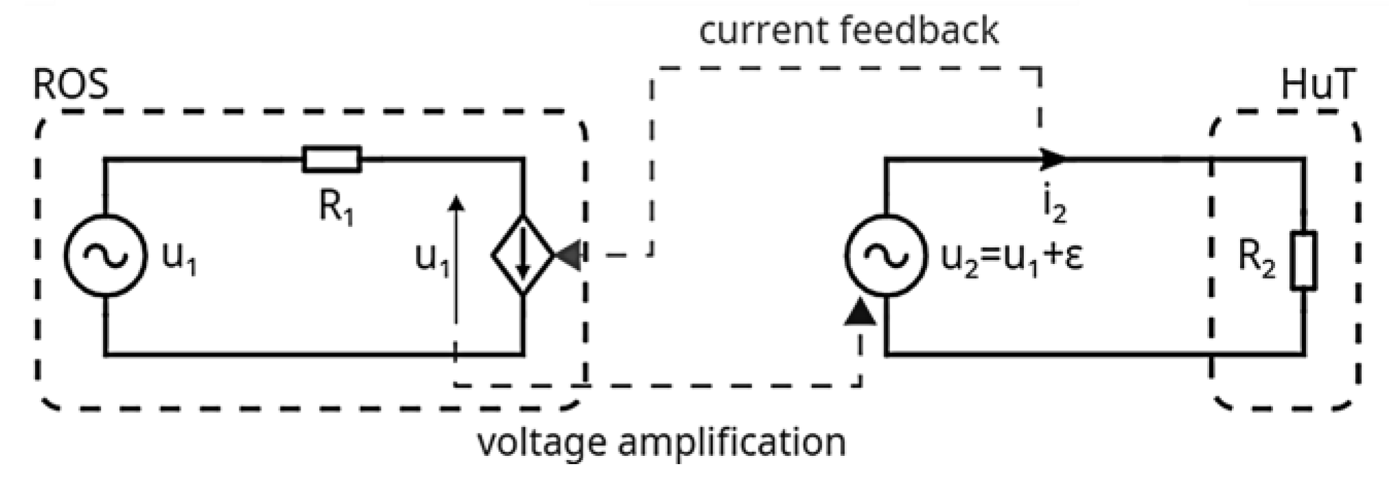
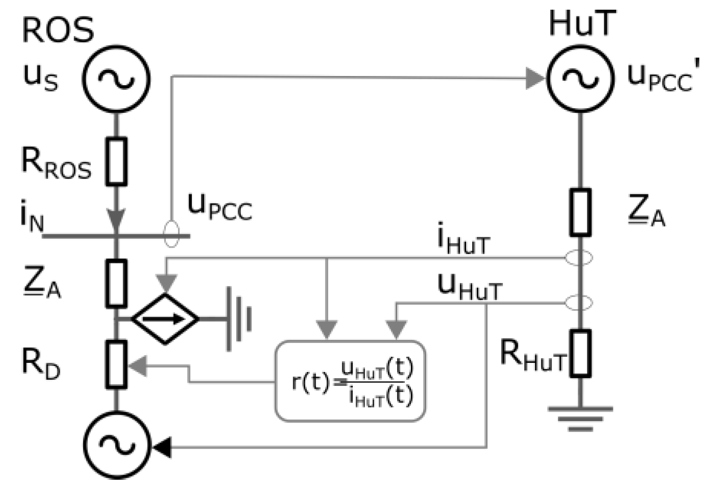
3.3. Hardware-in-the-Loop Real-Time Simulation Configuration

In recent years, RT simulation has become increasingly used together with Hardware-in-the-Loop (HiL) and its derivatives such as Controller-in-the-Loop (CiL) or Power-Hardware-in-the-Loop (PHiL) [38,39]. In the proposed DT application context, HiL is used to integrate measured and processed data into the RT simulation. In the HiL setup, the DTs are integrated with real components and controllers in a simulation environment. This enables the system to be tested under realistic conditions, with the RT feedback of the system’s performance. This feedback can be used to refine the DT models and to ensure an accurate representation of the physical behavior of the system. The principal idea of HiL coupling between simulation and components is shown in Figure 5.

In the proposed DT application, the voltage information is generated in the simulation, while the Rest-of-the-System (ROS) describes the grid and load configuration of the remaining grid. The Hardware-under-Test (HuT) is implemented as node DTs from the RTI. The voltage signal from the grid is fed into the HuT, and the resulting current feedback of the DT calculation is provided for the RT simulation.

A time-based coupling of these two independent systems can cause various types of negative effects, such as instability in the simulation part and oscillations between the systems. Different concepts of interface algorithms and compensation methods have been developed to address these phenomena [40,41,42]. Interface algorithms describe the handling of the data exchange between the simulation and the model or component part, considering a transfer function between the two systems. These algorithms ensure that the data exchange is done in a stable and efficient manner to prevent instabilities or oscillations. On the other hand, compensation methods are integrated into the simulation system itself to address possible oscillations. For example, one compensation method involves adding a damping factor to the simulation, reducing the oscillations’ magnitude.

An overview of different interface algorithms and compensation methods is provided in [43]. The “Variable Damping Impedance Method” (VDIM) was chosen to integrate DTs into the RT simulation. This method involves the use of an online processed damping factor to reduce oscillations and ensure stability. The principal structure and signal exchange for the VDIM is shown in Figure 6.

The VDIM approach involves the use of a feedback loop to adjust the damping factor based on the system’s current behavior. This ensures that the damping factor remains optimal for the current system condition and prevents oscillations and instabilities. Due to the knowledge about the grid node‘s active and reactive power, the damping impedance can be computed. As a result, this method is very well suited for the integration of DTs.

4. RTI Implementation into a Laboratory Test Bench

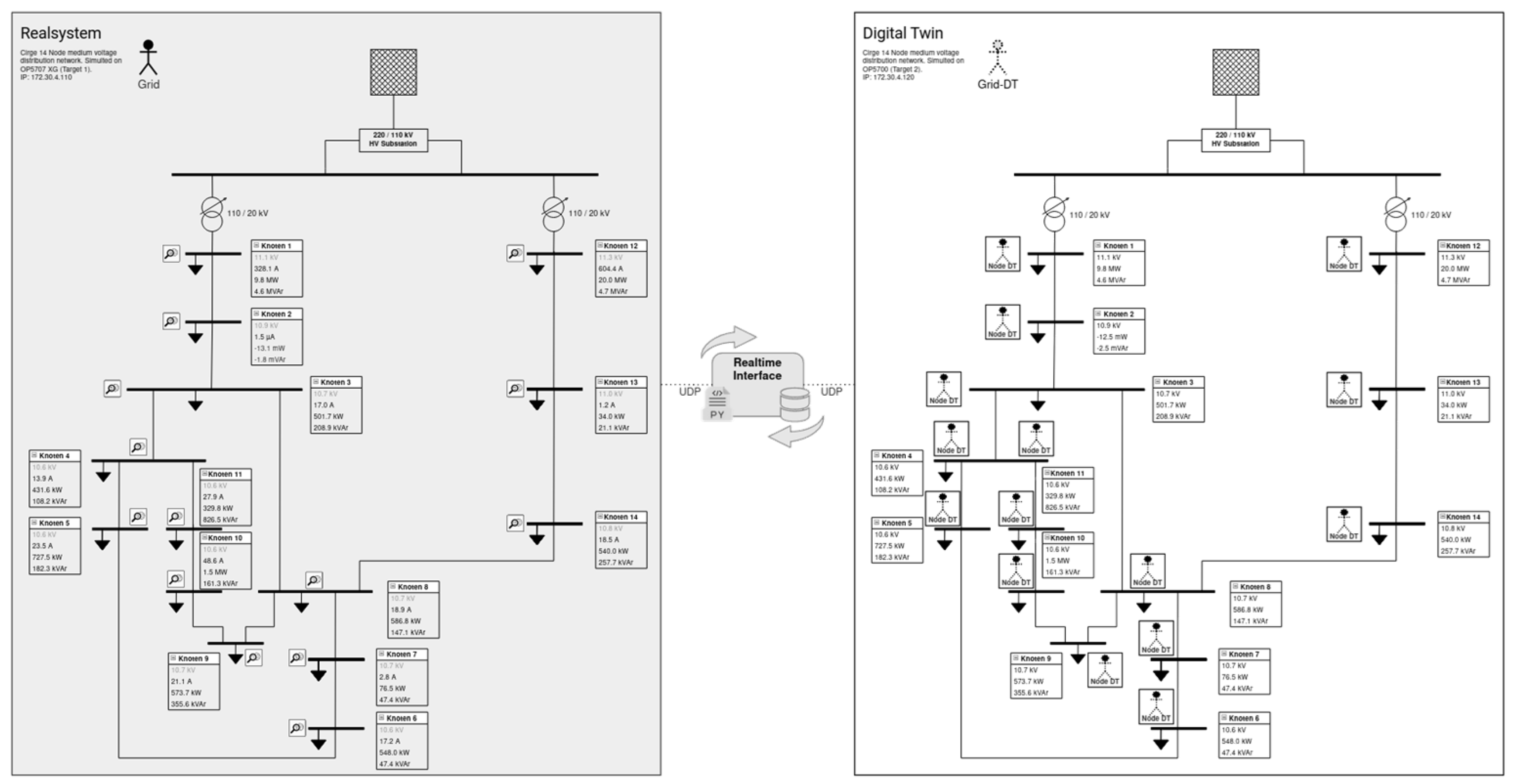
4.1. Simulation Setup

To develop, test, and validate the algorithms for the DT grid, a comprehensible and reproducible infrastructure was required. Therefore, a second RT simulation provided by Opal-RT was used to replace the physical grid as the leading system. This setup offered several advantages for development compared to modeling and measuring real grids. The main advantages were the presence of the same model basis in both systems, the possibilities of reproducible test scenarios, and the flexibility of the monitoring systems. Due to having the same model basis, documentation and modeling errors in the grid data could be avoided, and there was no need for an extensive process to correct errors in the grid basis. Furthermore, the simulation of the physical grid enabled the test of different and reproducible events, which cannot be introduced into the real grid. The flexible monitoring system allowed changes in measurement quality to test the stability of the system to signal and communication disturbances.

The additional simulator provided power signals transmitted as real measurements to the RTI and DT grid. These signals were generated by pre-processing functions within the RT simulation to produce the same data as real monitoring devices. This setup allowed testing of the DT grid as if it were connected to a real physical system. The following setup in Figure 7 shows the structure of the laboratory setup.

4.2. Grid Scenario and Focus of Investigations

To implement and test the hierarchical DT approach, an adapted variant of the European CIGRE MV distribution system [44] was modeled in the RT environment of Opal-RT with 50 µs step size. This test network provided sufficient control variables to test each part of the approach and could be evaluated in a comprehensible way due to the small number of nodes. The basic load and feed-in scenario was aligned from the parameterization in [44] and the results show sufficient accuracy. In addition, the operating and monitoring systems were made accessible via an external interface. The overall structure, integrated into a dashboard for displaying the data of the grid, is shown in Figure 8, for the physical grid simulation and the DT grid simulation.

Various simulations and tests were performed to validate the observer modeling, parameter estimation, HiL coupling, and overall performance of the hierarchical DTs. The tests were designed to evaluate the ability of the system to capture the behavior of the grid in different scenarios accurately.

First, the steady-state conditions between the leading simulation and the resulting grid DT were analyzed to verify the system’s principal functionality. Second, the dynamic behavior of the system was examined by introducing a load step at a single network node of the leading simulation and monitoring the voltage drop at the adjacent node. This allowed for an assessment of the ohmic-inductive voltage dependence of the load resulting in a corresponding load change, with voltage drops or rises.

The third focus of the tests was to evaluate the time delays in the calculation of the node DTs and the data transmission to the simulation. To do this, a UDP communication path was established between the leading and DT grid simulations. By introducing a voltage drop in the leading simulation and coupling it to a trigger signal via the second signal path, it was possible to measure the time delay between the direct-coupled trigger and the appearance of the event in the DT grid.

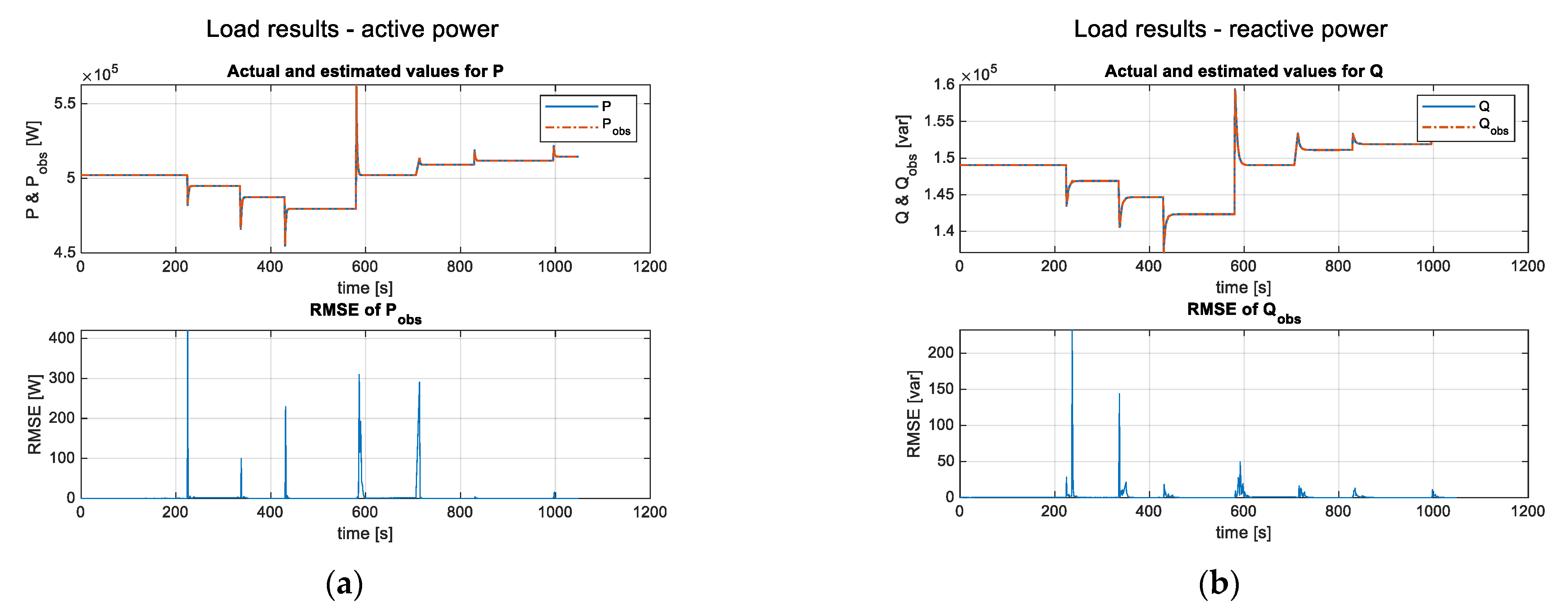
5. Results in Laboratory Setup

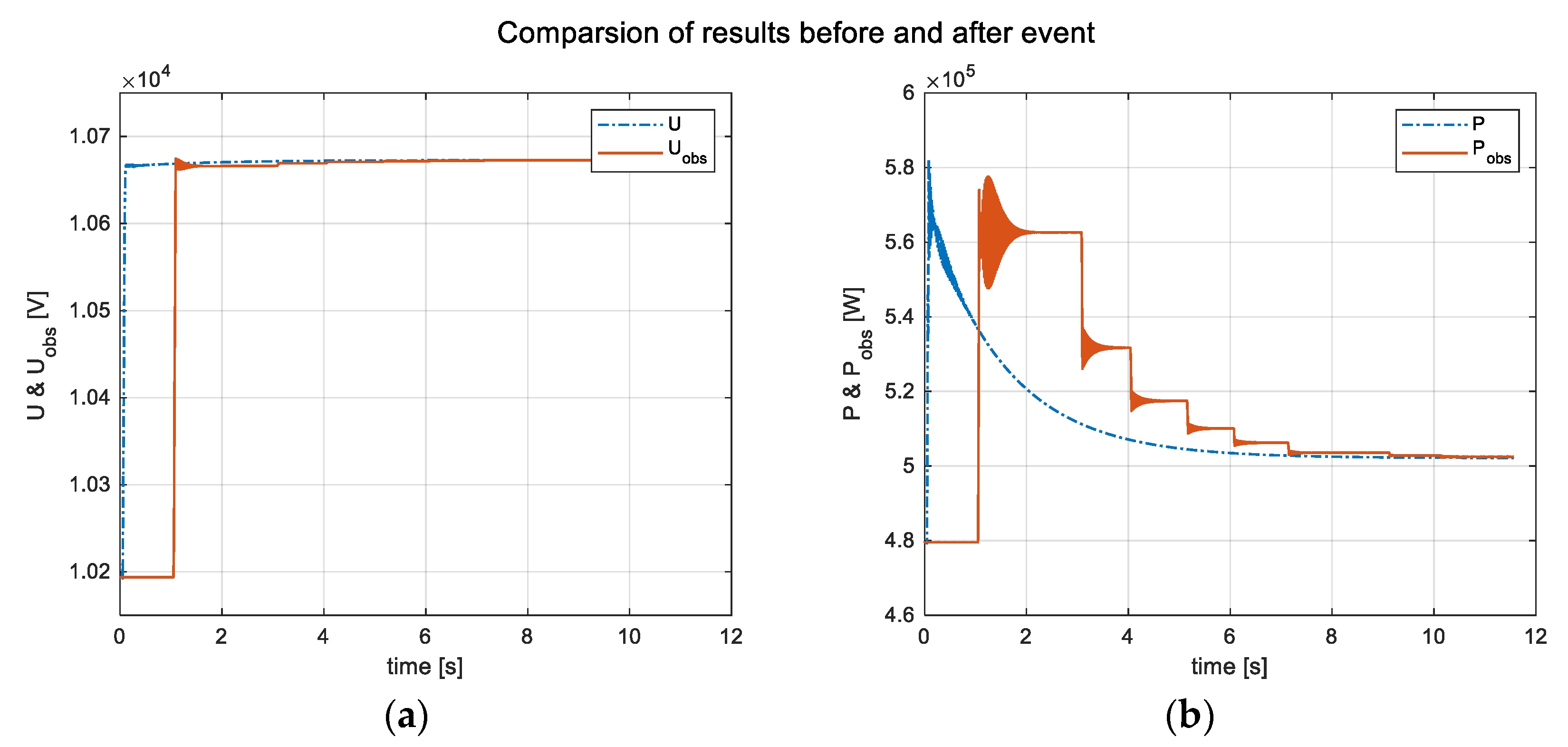
5.1. Results of the DT Grid: Steady-State Conditions

To investigate the DT grid’s general behavior and the simulation’s accuracy, steady-state conditions were compared between the physical grid simulation and the DT grid. The experimental test scenario started with a steady-state condition in both systems. The aim of the first test was to show the response of the grid nodes within both systems regarding a voltage increase. The event was triggered by a load drop at a neighboring node of the monitored node. Secondly, more grid scenarios were tested to validate that different loads and feed-ins were correctly aligned. To do this, the loads and feed-ins of the physical grid simulation were varied to generate voltage steps between +/− 10% of the nominal voltage. The behavior of both systems was recorded and compared.

First, Figure 9 shows the behavior in terms of active power in response to a voltage increase. The graphs show the active power and voltages of the grid node in the physical grid simulation and the observer-based DT grid.

The voltage signal results show a reasonable replication of the measured signals. After a delay of about 1 s, the model followed the leading signal and reached the steady state conditions. This implies that the load drop of the grid node to introduce the voltage event was tracked well. The active power signals also showed a good tracking of the steady-state conditions. Due to the ohmic-inductive behavior of the grid node, the power consumption went up with the increasing voltage. The estimated DT model could reproduce this behavior. The dynamic transition between the event and the steady state can be stepwise, which was also produced with the DT model. The oscillations in the P_obs signal occured due to the HiL coupling of the system and were an effect of the interface and time delays. The signal curve of P_obs showed a decrease in a stepped manner due to the HiL coupling and cycle times for the observer model. The simulation remained at the last setpoint until the new value was calculated and transmitted to the simulation. Depending on the time reference in the model, the cycle time of the observer must be varied. In terms of steady-state conditions, the oscillations and stepped decrease were insignificant for the overall results. For integrating high bandwidth data, like harmonics, the interface algorithms must be extended to compensate for these effects. The voltage and model behavior of the system showed an exemplary mapping of the original system state. The voltage drop followed the leading signal with a short time delay. The steady-state condition of the DT grid equaled the physical grid simulation.

Second, Figure 10 shows the active and reactive power of the measured signals and the observer’s results in terms of the active and reactive power for the different setpoints on a single grid node.

The results of the different scenarios show that the condition of each grid state was calculated. The Kalman filter correctly estimated the parameters of the model to reproduce the active and reactive power. The steady-state conditions complied for every scenario with the values of the physical grid. The estimated values for the node-specific DTs also showed the same response in the transition period between the event and steady state in the DT grid simulation. The root-mean-square-error (RMSE) between the physical grid simulation and the observer-based DT grid shows temporary deviations between both measurements. Error spikes can be seen at the beginning of the steps, which result from the HiL-coupled RT simulation. Due to the interface algorithm, the error spikes reduce fast to zero and are insignificant compared to the connected powers of the nodes.

Overall, the analysis of the simulations shows promising results in terms of reproducing the steady-state conditions. Each grid node’s active and reactive power could be reproduced in the DT grid simulation. In addition, the voltages of the DT grid simulation follow the measurements of the physical grid simulation.

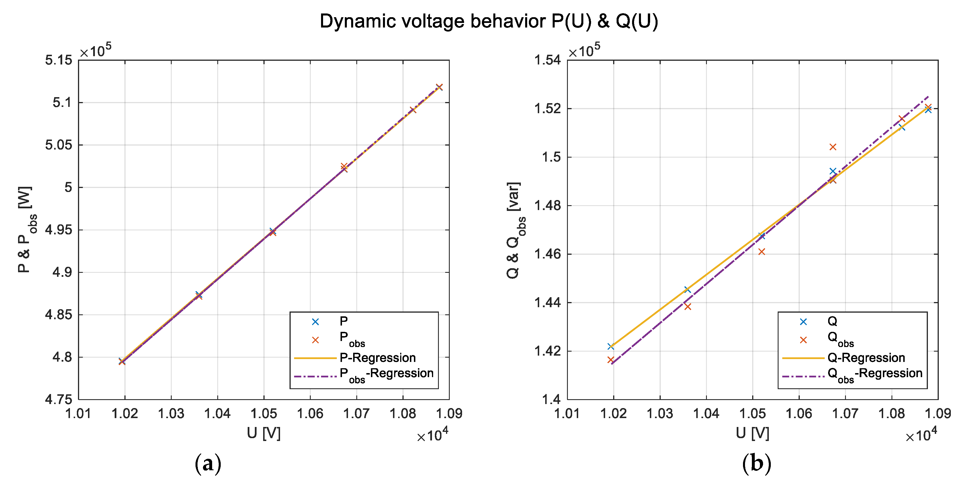
5.2. Results of the DT Grid: Dynamic Behavior

The dynamic behavior of the grid node in terms of voltage dependency for active and reactive power is a key component of the system. To track this behavior, the DT can provide information beyond standard measurements and can calculate more details on the grid state.

The test scenario also started with steady-state conditions in both systems. The implementation of the physical grid simulation included a configuration for the dynamic load behavior P(U) and Q(U). To test the parameter estimation of the Kalman filter, a voltage drop at a neighboring node was introduced into the system. As a result, the observed load changed the active and reactive power value according to the voltage dependence. The voltage event was varied around the nominal voltage to generate a characteristic of the model’s behavior. The behavior of both systems was recorded and evaluated.

The following Figure 11 shows the dependency P(U) und Q(U) for the physical grid simulation and the observer model.

The graph for the active power indicates a perfect match between the measured and estimated values. The active power change was nearly the same for every voltage variation in both simulations. The deviations between the configured and the observed load are at a minimum level. Considering the regression between the setpoints, nearly no deviation is noticeable. The reactive power results also show suitable matches, especially around the nominal voltage. The deviations rise with increasing or decreasing voltage of the system.

Overall, the estimation of system dynamics with the Kalman filter shows realistic values to track the system behavior. The estimated parameters can rebuild the characteristics of the monitored grid node. An issue that can arise is that there is a need to match the global parameters of the dynamic behavior to the measured system. The estimated parameters fit the dynamic characteristics of the physical grid nodes, but it is questionable that these values are the globally correct values. The tested scenarios allowed the assumption that the estimated values were in the range of the real values. Further development must be done to ensure the values can come as near as possible to the real characteristics. A possible solution to obtain a more secure parameter set is the integration of intelligent limits for each model parameter. This could be based on prior knowledge of the loads and feed-ins of the underlying grid, or could be processed during operation.

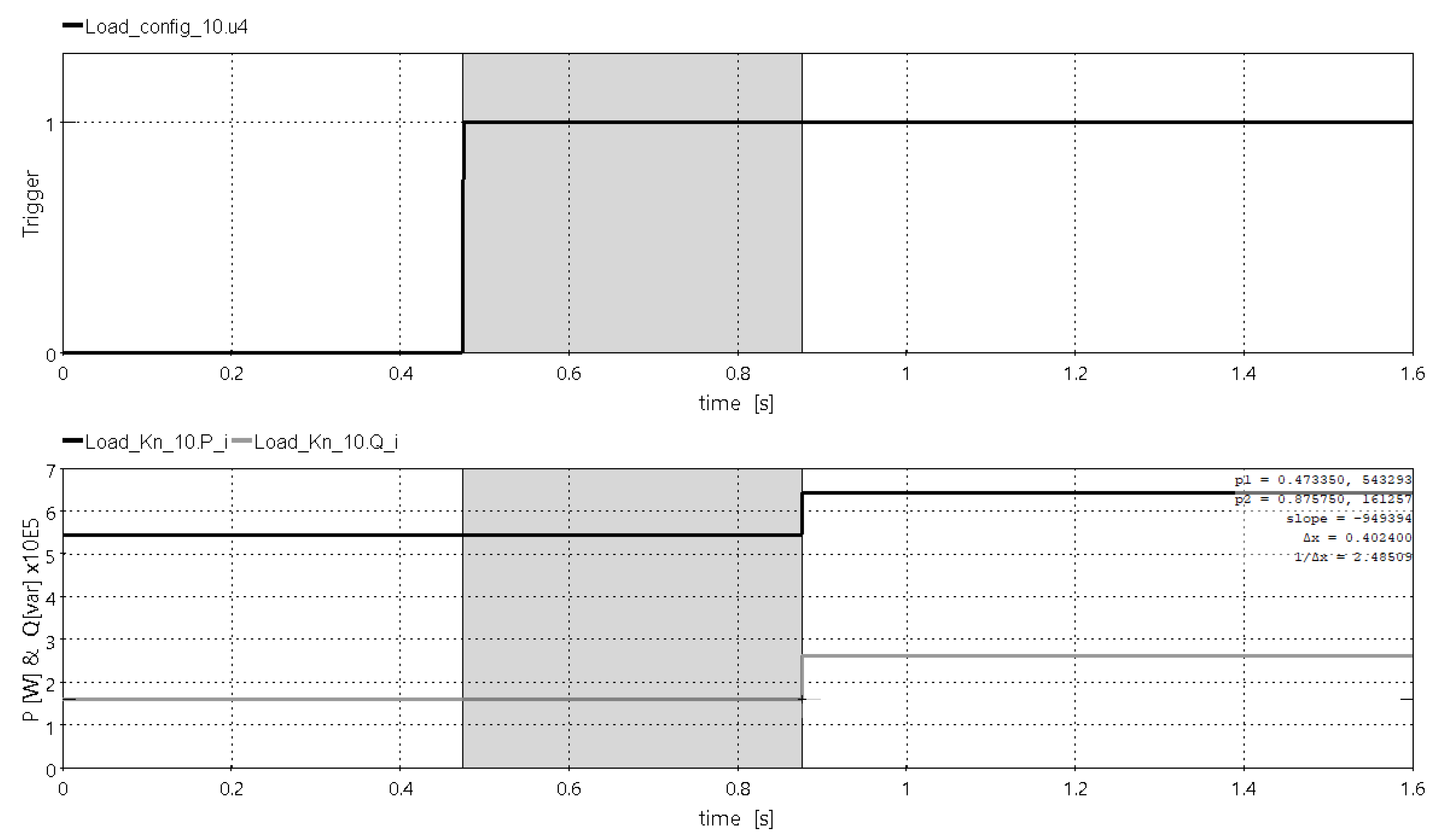
5.3. Time Delays for Communication and Processing Grid Information

Another important system parameter is the cycle time of the RTI. This time represents the complete data acquisition, transmission, and processing process between the measurement in the physical grid and the forwarding of the value into the DT grid simulation. An additional trigger signal was set via a UDP connection between the physical grid simulation and the DT grid to measure this system parameter. The physical grid simulation sends the trigger signal at the exact same time when a load change occurs. Figure 12 shows the reception of the trigger signal (upper graph) and power signals (lower graph), both measured at the DT grid simulation.

The time delay of the signals was measured between the rising edges of both signals. The measured time delay between the physical grid simulation and the DT grid for this signal exchange corresponds to 402.2 ms. This time delay varied between ~350 ms and ~500 ms during the simulation. The variations occurred due to the calculation times of the parameter estimation and the further processes within the RTI. The lower graph shows the values for active and reactive power of one grid node; both signals are received and processed in the simulation during the same time step. This applies to all other input signals of the DT grid simulation. Therefore, it can be assumed that the communication does not introduce any additional delays between the individual signals.

Process times are a limiting factor in scaling the system to analyze grids with large extents and large numbers of nodes. Two factors must be considered when determining the DT for these grids. First, the simulation time within the RT simulation must be smaller than the time step itself. To ensure this, it is necessary to make sure that sufficient computing power is available to simulate the network. By calculating the node behavior in the RTI, the required simulation time is slightly reduced, because the simulation does not have to process the model parameters itself. Second, the processing time in the RTI must be suitable to update the model parameters faster than the time basis of modeled characteristic. Since the observer computation is a parallel process, it is scalable to large grids, assuming the base system has sufficient processing power.

6. Conclusions

Fundamental changes in energy production, distribution, and consumption drive the transformation of the energy system. Distribution grids are facing this transformation due to the increasing penetration of renewable energy sources and the changing load characteristics resulting from the transformation of the mobility and heating sectors. There is a growing need for digitalization and automation in distribution networks to meet these challenges. This can enable more efficient and reliable distribution grid management, along with better monitoring and control of the assets. Grid transparency features regarding monitoring, load and feed-in characteristics, and topology are key features to support future energy transmission and distribution systems. The Digital Twin approach combines system data with online measurements to create a digital replica of the physical system.

The developed hierarchical Digital Twin of a distribution system describes the transfer of the actual grid state into an online coupled RT simulation. The result is a Digital Twin grid simulation that reflects the behavior of the physical grid. Based on measured data, local clients densify the grid state in the field and provide it for further calculations to match the dynamic behavior. In preparation for the simulation, node-specific Digital Twins were developed to capture the dynamic behavior of each node. The parameters of the exponential recovery load model were estimated using Kalman filters to track the voltage dependence characteristics in the Digital Twin grid simulation. A Hardware-in-the-Loop setup was established to connect the Digital Twin nodes into a vendor-agnostic RT simulation system. The resulting Digital Twin grid processed the node information with RT simulation, providing a powerful platform for monitoring, testing, and validating grid automation and commissioning to assist grid operation and planning.

The developed system was tested in different validation setups to evaluate the results regarding overall steady-state replication, tracking of dynamic behavior, and time delays between the physical grid and the Digital Twin grid simulation. To provide initial traceable data, the lab setup included a second RT platform that replaced the grid monitoring and feds the system with grid information. The results of the investigations show an excellent replication of the real system. Steady-state conditions were transferred with minimal deviation. The time delay between the physical grid simulation and the Digital Twin grid simulation varied between ~350 ms and ~500 ms, which is fast enough to provide data for SCADA systems. Regarding the dynamic voltage dependence of grid nodes, the results indicate good replication for the system parameter estimated with the Kalman filter. The characteristics of active and reactive power can be mapped and compared with the input data of the leading simulation, and only minor differences were found. Further developments are forthcoming, as we intend to reflect on the issues about a global parameter set of estimation with the Kalman filter by adding more information about the system. Furthermore, the model basis will be increased to include more specific behavior of the grid nodes in Digital Twins.

References

1. Tuttokmagi, O.; Kaygusuz, A. Smart Grids and Industry 4.0. In Proceedings of the 2018 International Conference on Artificial Intelligence and Data Processing (IDAP), Malatya, Turkey, 28–30 September 2018; pp. 1–6. [Google Scholar]
2. IEC 61850:2022; Communication Networks and Systems for Power Utility Automation-ALL PARTS. IEC: London, UK, 2022.
3. IEC 60870-5-104:2006+AMD1:2016; Telecontrol Equipment and Systems—Part 5-104: Transmission Protocols—Network Access for IEC 60870-5-101 Using Standardtransport Profiles. IEC: London, UK, 2016.
4. Rösch, D.; Kummerow, A.; Ruhe, S.; Schäfer, K.; Monsalve, C.; Nicolai, S. IT-Sicherheit in digitalen Stationen: Cyber-physische Systemmodellierung, -bewertung und -analyse. Automatisierungstechnik 2020, 68, 720–737. [Google Scholar] [CrossRef]
5. Rinaldi, S.; Ferrari, P.; Ali, N.M.; Gringoli, F. IEC 61850 for micro grid automation over heterogeneous network: Requirements and real case deployment. In Proceedings of the 2015 IEEE 13th International Conference on Industrial Informatics (INDIN), Cambridge, UK, 22–24 July 2015; pp. 923–930. [Google Scholar]
6. Uluski, R.W. The role of Advanced Distribution Automation in the Smart Grid. In Proceedings of the IEEE PES General Meeting, Minneapolis, MN, USA, 25–29 July 2010; pp. 1–5. [Google Scholar]
7. Dileep, G. A survey on smart grid technologies and applications. Renew. Energy 2020, 146, 2589–2625. [Google Scholar] [CrossRef]
8. Ratnam, K.S.; Palanisamy, K.; Yang, G. Future low-inertia power systems: Requirements, issues, and solutions—A review. Renew. Sustain. Energy Rev. 2020, 124, 109773. [Google Scholar] [CrossRef]
9. Ferrari, M.; Orendorff, M.; Smith, T.; Buckner, M.A. Open-Code, Real-Time Emulation Testbed OF Grid-Connected Type-3 Wind Turbine System with Hardware Validation. In Proceedings of the 2019 IEEE Applied Power Electronics Conference and Exposition (APEC), Anaheim, CA, USA, 17–21 March 2019; pp. 66–70. [Google Scholar]
10. Hashimoto, J.; Ustun, T.S.; Suzuki, M.; Sugahara, S.; Hasegawa, M.; Otani, K. Advanced Grid Integration Test Platform for Increased Distributed Renewable Energy Penetration in Smart Grids. IEEE Access 2021, 9, 34040–34053. [Google Scholar] [CrossRef]
11. Wagle, R.; Tricarico, G.; Sharma, P.; Sharma, C.; Rueda, J.L.; Gonzalez-Lonzatt, F. Cyber-Physical Co-Simulation Testbed for Real-Time Reactive Power Control in Smart Distribution Network. In Proceedings of the 2022 IEEE PES Innovative Smart Grid Technologies—Asia (ISGT Asia), Singapore, 1–5 November 2022; pp. 11–15. [Google Scholar]
12. Onile, A.E.; Machlev, R.; Petlenkov, E.; Levron, Y.; Belikov, J. Uses of the digital twins concept for energy services, intelligent recommendation systems, and demand side management: A review. Energy Rep. 2021, 7, 997–1015. [Google Scholar] [CrossRef]
13. Rasheed, A.; San, O.; Kvamsdal, T. Digital Twin: Values, Challenges and Enablers From a Modeling Perspective. IEEE Access 2020, 8, 21980–22012. [Google Scholar] [CrossRef]
14. Jacoby, M.; Usländer, T. Digital Twin and Internet of Things—Current Standards Landscape. Appl. Sci. 2020, 10, 6519. [Google Scholar] [CrossRef]
15. Arrano-Vargas, F.; Konstantinou, G. Modular Design and Real-Time Simulators Toward Power System Digital Twins Implementation. IEEE Trans. Ind. Inf. 2023, 19, 52–61. [Google Scholar] [CrossRef]
16. Cioara, T.; Anghel, I.; Antal, M.; Antal, C.; Arcas, G.I.; Croce, V. An Overview of Digital Twins Application in Smart Energy Grids. In Proceedings of the 2022 IEEE 18th International Conference on Intelligent Computer Communication and Processing (ICCP), Cluj-Napoca, Romania, 22–24 September 2022; pp. 25–30. [Google Scholar]
17. Bazmohammadi, N.; Madary, A.; Vasquez, J.C.; Mohammadi, H.B.; Khan, B.; Wu, Y.; Guerrero, J.M. Microgrid Digital Twins: Concepts, Applications, and Future Trends. IEEE Access 2022, 10, 2284–2302. [Google Scholar] [CrossRef]
18. Brosinsky, C.; Westermann, D.; Krebs, R. Recent and prospective developments in power system control centers: Adapting the digital twin technology for application in power system control centers. In Proceedings of the 2018 IEEE International Energy Conference (ENERGYCON), Limassol, Cyprus, 3–7 June 2018; pp. 1–6. [Google Scholar]
19. Ruhe, S.; Nicolai, S.; Bretschneider, P.; Westermann, D. Real-Time Approach of Grid-Parallel Simulation for Automated Distribution Grids. In Proceedings of the 2022 57th International Universities Power Engineering Conference (UPEC), Istanbul, Turkey, 30 August–2 September 2022; pp. 1–6. [Google Scholar]
20. Monsalve, C.; Alramlawi, M.; Ruhe, S.; Schaefer, K.; Nicolai, S.; Bretschneider, P. A Novel Framework Architecture for Distributed Digital Twins in Power Systems. In Proceedings of the ETG Congress 2021, Online, 18–19 March 2021; pp. 1–6. [Google Scholar]
21. Yang, Y.; Chen, Z.; Yan, J.; Xiong, Z.; Zhang, J.; Yuan, H.; Tu, Y.; Zhang, T. State Evaluation of Power Transformer Based on Digital Twin. In Proceedings of the 2019 IEEE International Conference on Service Operations and Logistics, and Informatics (SOLI), Zhengzhou, China, 6–8 November 2019; pp. 230–235. [Google Scholar]
22. Kuber, S.; Sharma, M.; Bonetti, A.; Harispuru, C.; Soroush, A. Virtual Testing of Protection Systems using Digital Twin Technology. In Proceedings of the 2022 75th Annual Conference for Protective Relay Engineers (CPRE), College Station, TX, USA, 25–28 May 2022; pp. 1–8. [Google Scholar]
23. Sleiti, A.K.; Kapat, J.S.; Vesely, L. Digital twin in energy industry: Proposed robust digital twin for power plant and other complex capital-intensive large engineering systems. Energy Rep. 2022, 8, 3704–3726. [Google Scholar] [CrossRef]
24. Brosinsky, C.; Krebs, R.; Westermann, D. Embedded Digital Twins in future energy management systems: Paving the way for automated grid control. Automatisierungstechnik 2020, 68, 750–764. [Google Scholar] [CrossRef]
25. Thomas, M.S.; McDonald, J.D. Power System SCADA and Smart Grids; CRC Press: Boca Raton, FL, USA, 2015. [Google Scholar]
26. Huang, Y.-F.; Werner, S.; Huang, J.; Kashyap, N.; Gupta, V. State Estimation in Electric Power Grids: Meeting New Challenges Presented by the Requirements of the Future Grid. IEEE Signal Process. Mag. 2012, 29, 33–43. [Google Scholar] [CrossRef] [Green Version]
27. Yang, C.-W.; Dubinin, V.; Vyatkin, V. Automatic Generation of Control Flow from Requirements for Distributed Smart Grid Automation Control. IEEE Trans. Ind. Inf. 2020, 16, 403–413. [Google Scholar] [CrossRef]
28. Gungor, V.C.; Sahin, D.; Kocak, T.; Ergut, S.; Buccella, C.; Cecati, C.; Hancke, G.P. A Survey on Smart Grid Potential Applications and Communication Requirements. IEEE Trans. Ind. Inf. 2013, 9, 28–42. [Google Scholar] [CrossRef] [Green Version]
29. Ruhe, S.; Nicolai, S.; Jiang, T.; Cai, H.; El Sayed, N.; Geithner, T.; Frueh, N.; Ulbig, A.; Schoenfeld, B.; Prinz, S. Approach of a DT based automatic grid operation for distribution grids. In Proceedings of the ETG Congress 2021, Online, 18–19 March 2021; pp. 1–6. [Google Scholar]
30. Faruque, M.O.; Strasser, T.; Lauss, G.; Jalili-Marandi, V.; Forsyth, P.; Dufour, C.; Dinavahi, V.; Monti, A.; Kotsampopoulos, P.; Martinez, J.A.; et al. Real-Time Simulation Technologies for Power Systems Design, Testing, and Analysis. IEEE Power Energy Technol. Syst. J. 2015, 2, 63–73. [Google Scholar] [CrossRef]
31. Guillaud, X.; Faruque, M.O.; Teninge, A.; Hariri, A.H.; Vanfretti, L.; Paolone, M.; Dinavahi, V.; Mitra, P.; Lauss, G.; Dufour, C.; et al. Applications of Real-Time Simulation Technologies in Power and Energy Systems. IEEE Power Energy Technol. Syst. J. 2015, 2, 103–115. [Google Scholar] [CrossRef] [Green Version]
32. Madhuri, D.; Reddy, P.C. Performance comparison of TCP, UDP and SCTP in a wired network. In Proceedings of the 2016 International Conference on Communication and Electronics Systems (ICCES), Coimbatore, India, 21–22 October 2016; pp. 1–6. [Google Scholar]
33. Pasiopoulou, I.D.; Kontis, E.O.; Papadopoulos, T.; Papagiannis, G.K. Effect of load modeling on power system stability studies. Electr. Power Syst. Res. 2022, 207, 107846. [Google Scholar] [CrossRef]
34. Arif, A.; Wang, Z.; Wang, J.; Mather, B.; Bashualdo, H.; Zhao, D. Load Modeling—A Review. IEEE Trans. Smart Grid 2018, 9, 5986–5999. [Google Scholar] [CrossRef]
35. Karlsson, D.; Hill, D.J. Modelling and identification of nonlinear dynamic loads in power systems. IEEE Trans. Power Syst. 1994, 9, 157–166. [Google Scholar] [CrossRef] [Green Version]
36. Wan, E.A.; van der Merwe, R. The unscented Kalman filter for nonlinear estimation. In Proceedings of the IEEE 2000 Adaptive Systems for Signal Processing, Communications, and Control Symposium (Cat. No.00EX373), Lake Louise, AB, Canada, 4 October 2000; pp. 153–158. [Google Scholar]
37. Rouhani, A.; Abur, A. Real-Time Dynamic Parameter Estimation for an Exponential Dynamic Load Model. IEEE Trans. Smart Grid 2016, 7, 1530–1536. [Google Scholar] [CrossRef]
38. Edrington, C.S.; Steurer, M.; Langston, J.; El-Mezyani, T.; Schoder, K. Role of Power Hardware in the Loop in Modeling and Simulation for Experimentation in Power and Energy Systems. Proc. IEEE 2015, 103, 2401–2409. [Google Scholar] [CrossRef]
39. Resch, S.; Friedrich, J.; Wagner, T.; Mehlmann, G.; Luther, M. Stability Analysis of Power Hardware-in-the-Loop Simulations for Grid Applications. Electronics 2022, 11, 7. [Google Scholar] [CrossRef]
40. Lentijo, S.; D’Arco, S.; Monti, A. Comparing the Dynamic Performances of Power Hardware-in-the-Loop Interfaces. IEEE Trans. Ind. Electron. 2010, 57, 1195–1207. [Google Scholar] [CrossRef]
41. Brandl, R. Operational Range of Several Interface Algorithms for Different Power Hardware-in-the-Loop Setups. Energies 2017, 10, 1946. [Google Scholar] [CrossRef] [Green Version]
42. Hatakeyama, T.; Riccobono, A.; Monti, A. Stability and accuracy analysis of power hardware in the loop system with different interface algorithms. In Proceedings of the 2016 IEEE 17th Workshop on Control and Modeling for Power Electronics (COMPEL), Trondheim, Norway, 27–30 June 2016; pp. 1–8. [Google Scholar]
43. Ruhe, S.; Fechner, M.; Nicolai, S.; Bretschneider, P. Simulation of Coupled Components within Power-Hardware-in-the-Loop (PHiL) Test Bench. In Proceedings of the 2020 55th International Universities Power Engineering Conference (UPEC), Torino, Italy, 1–4 September 2020; pp. 1–6. [Google Scholar]
44. Rudion, K.; Orths, A.; Styczynski, A.; Strunz, K. Design of benchmark of medium voltage distribution network for investigation of DG integration. In Proceedings of the 2006 IEEE Power Engineering Society General Meeting, Montreal, QC, Canada, 18–22 June 2006; p. 6. [Google Scholar]
Figure 1. Hierarchical DT infrastructure and communication setup.
Electronics 12 02747 g001
Figure 2. Principal HiL setup for coupling node DTs to RT simulation.
Electronics 12 02747 g002
Figure 3. Real-time interface components and signal exchange.
Electronics 12 02747 g003
Figure 4. Communication setup with database integration.
Electronics 12 02747 g004
Figure 5. Principal concept of Hardware-in-the-Loop simulations; Rest-of-the-System (ROS), Hardware-under-Test (HuT).
Electronics 12 02747 g005
Figure 6. Principle structure “Variable Damping Impedance Method”.
Electronics 12 02747 g006
Figure 7. Simulation setup with leading RT simulation to emulate the physical grid.
Electronics 12 02747 g007
Figure 8. Implementation of CIGRE 14 node MV benchmark grid in leading and DT grid simulation.
Electronics 12 02747 g008
Figure 9. Results of active power consumption (b) following a voltage increase (a) for measured values of the simulated physical grid (P, U) and the DT grid (Pobs, Uobs).
Electronics 12 02747 g009
Figure 10. Results of active (a) and reactive (b) power for simulated physical grid (P, U) and the DT grid (Pobs, Uobs).
Electronics 12 02747 g010
Figure 11. Results of the calculation for the dynamic behavior of the grid nodes for active power (a) and reactive power (b).
Electronics 12 02747 g011
Figure 12. Time delay between trigger signal (up) from physical grid simulation and related signal input in DT grid (down).
Electronics 12 02747 g012
Disclaimer/Publisher’s Note: The statements, opinions and data contained in all publications are solely those of the individual author(s) and contributor(s) and not of MDPI and/or the editor(s). MDPI and/or the editor(s) disclaim responsibility for any injury to people or property resulting from any ideas, methods, instructions or products referred to in the content.