Article

Identification of Indoor Radio Environment Properties from Channel Impulse Response with Machine Learning Models

by
Teodora Kocevska
1,2,*,
Tomaž Javornik
1,2,
Aleš Švigelj
1,2,
Aleksandra Rashkovska
1 and
Andrej Hrovat
1,2
1
Department of Communication Systems, Jožef Stefan Institute, Jamova Cesta 39, SI-1000 Ljubljana, Slovenia
2
Jožef Stefan International Postgraduate School (IPS), Jamova Cesta 39, SI-1000 Ljubljana, Slovenia
*
Author to whom correspondence should be addressed.
Electronics 2023, 12(12), 2746; https://doi.org/10.3390/electronics12122746
Submission received: 12 May 2023 / Revised: 9 June 2023 / Accepted: 17 June 2023 / Published: 20 June 2023
(This article belongs to the Section Microwave and Wireless Communications)

Abstract

:
The design and optimization of next-generation indoor wireless communication networks require detailed and precise descriptions of the indoor environments. Environmental awareness can serve as a fundamental basis for the dynamic adaptation of the wireless system to channel conditions and can improve the system’s performance. Methods that combine wireless technology with machine learning are promising for identifying the properties of the indoor radio environment (RE) without requiring specialized equipment or manual intervention. In the paper, we propose an approach for identifying the materials of the surfaces using channel impulse response (CIR) and RE identification models built with machine learning. To train the models and assess their performance, we acquired radio propagation data from rooms with different sizes and materials using ray tracing. We explored tree-based methods, ensemble-based methods, kernel-based methods, and neural networks for training the models. The performance of the models is evaluated in three realistic scenarios defined by the location of the radio nodes and the room sizes. The multilayer perceptron models performed best in most of the evaluation settings. The results show that the models are capable of accurately predicting the materials in rooms with sizes that were not included in the training procedure. Including CIRs from a large number of rooms with different sizes and surface materials estimated with different radio node positions in the training process results in models with wider practical applicability.

1. Introduction

The investigation of channel characteristics is crucial for wireless systems to meet the requirements of the wide range of emerging applications [1]. The radio environment (RE) significantly affects the performance of wireless communication systems. While the outdoor propagation environment is well described by digital elevation models and terrain usage data, accurate and up-to-date information about the indoor propagation environment is not ubiquitously available. Therefore, automatic and seamless characterization is mandatory for introducing environment-aware wireless communications [2] and for creating and continually updating the digital twin of the building [3]. Enhanced environmental awareness can be applied for the design and optimization of next-generation wireless systems and the development of methods for dynamic adaptation of a wireless system to the channel conditions [4], but also in emerging applications related to navigation [5], localization [6], emergency response [7], and automation in smart buildings [8].
The conventional methods for estimating indoor RE [9] are not adequate for automatic characterization of the indoor propagation environment because they are implemented by means of specialized, complex, and expensive equipment and involve human and/or robot participation. Additionally, the information about the environment provided by these methods is limited and does not provide insight into the properties that affect the electromagnetic waves propagating between the transmitter and receiver (e.g., the roughness of the surfaces and the electromagnetic properties of the materials).
Environment characterization with machine learning techniques [10,11] can provide alternative solutions to the bottlenecks in conventional methods. Advancements in wireless communications and machine learning offer an unprecedented opportunity for wireless sensing [12,13] and intelligent environment identification [14]. The received signal conveys information about the surroundings, and a mapping between the propagation characteristics and the propagation environment exists. Machine learning techniques have been shown to have good performance in modeling the correlation between the input and output features using large training databases [15,16,17]. Thus, it is envisioned to be appropriate to learn accurate predictive models to identify the properties of the propagation environment. The massive number of wireless devices deployed indoors will provide abundant radio propagation data from various buildings, communication technologies, and frequencies needed for training the models.
In our previous work, we started research in the joint use of wireless signals and machine learning models for the characterization of indoor geometry and the materials of the surfaces, and we published the idea, first concepts, and preliminary results. We introduced the idea of using radio scanning for three-dimensional characterization of an indoor environment in [18]. To validate the proposed approach, we specified a basic set of propagation characteristics of the multipath components (MPCs) as features of the RE signature, and we formalized an initial framework that enables the identification of the material of a single wall [19]. In [20], we evaluated the material identification using a baseline data set. Motivated by the promising results of our early studies, we extended our research to the identification of multiple properties of the propagation environment.
In this article, we focus on the limitations of the approach proposed in our previous work, namely, (i) the characterization of a single wall material in a room, while in modern buildings different materials are used for inner and outer walls, ceilings, and floors, (ii) the initial model is built and validated for a single room size while in reality the rooms are of different sizes, and (iii) the assumption of the same set of link positions for training and testing while in practice the same link position may be impossible to fulfill. In this respect, we introduce an extended methodology that enables the identification of the properties of all of the surfaces in the room. The methodology is evaluated for the identification of the materials in plain rooms. We propose a supervised identification that requires a training procedure for constructing predictive models using spatially distributed channel impulse responses (CIRs) labeled with the materials of the surfaces as training data. An individual predictive model is trained to identify the presence/absence of a material. We investigate the impact of the locations of the radio nodes and the room sizes considered in the training procedure on the performance of the models when applied to data from different radio links and rooms. The main contributions of this study are summarized as follows:
  • An extended data-driven methodology for identification of the properties of all surfaces in an indoor propagation environment based on CIR;
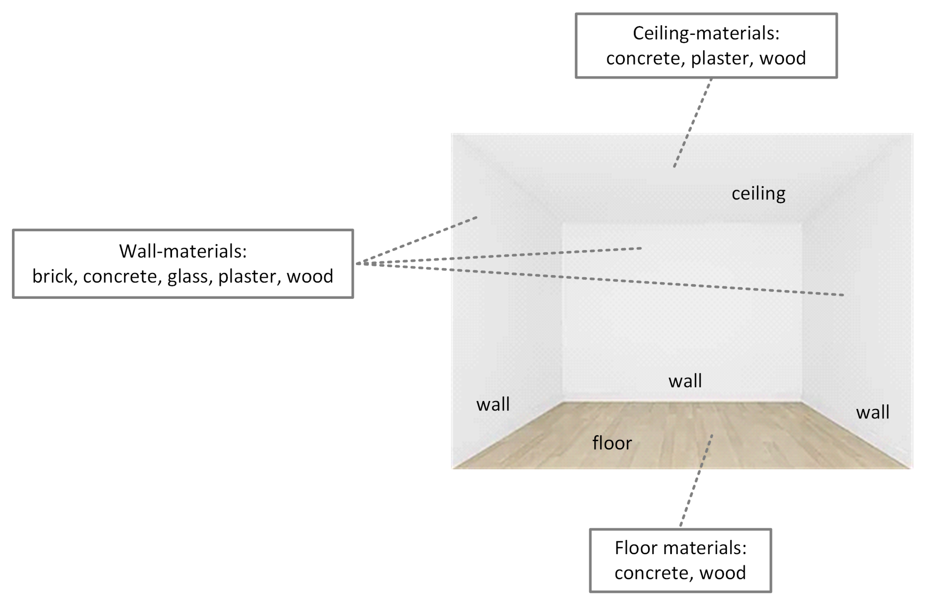
  • Validation of the proposed methodology for identification of all the materials used for the surfaces in the room;
  • Evaluation of the identification performance of the models in three scenarios and analysis of the impact of the radio nodes’ locations and room sizes considered in the training phase on the model’s applicability;
  • Open access data set containing indoor radio propagation data from a large number of rooms annotated with the location of the radio node, the room’s geometry, and the surfaces’ materials.
The remainder of the paper is organized as follows. An overview of the related work on indoor environment characterization is given in Section 2. We introduce the concept of data-driven indoor environment identification and describe the methodology in detail in Section 3. The procedure for evaluating the proposed methodology for the identification of the materials is presented in Section 4. This section provides elaboration on the learning task, learning approach, procedure for CIR acquisition, evaluation scenarios, and the metrics for assessing performance. Section 5 reports the results and discusses the identification performance. Finally, we conclude the paper and suggest directions for future work in Section 6.

2. Related Work

The machine-learning-enabled identification of the indoor environment has only recently attracted research attention, mainly in the last few years. Therefore, the topic has scarcely been studied, with just a few studies published in the literature [10]. The methods for determining the properties of indoor surfaces based on machine learning and CIR have not been widely studied to the authors’ knowledge. The publications that have studied the use of machine learning for the identification of the indoor scenario [21,22] consider the propagation environment as a whole and do not investigate the identification of the properties of the surfaces that bound the space. The characterization of materials samples has been researched using various methods, such as the coaxial probe method, free space measurement, and resonant, to name a few [23]. Several conventional studies have made on-site measurements of the reflection coefficient and estimated the relative permittivity of the materials based on the reflection loss [24,25,26]. Recently, the inverse reflection problem was combined with the identification of the reflecting surfaces from a point cloud to obtain a three-dimensional permittivity map of an empty office environment at 60 GHz [27]. Due to the use of high-quality equipment, the need for manual intervention, and the high cost, these methods are not best suited for the fast characterization needed for the digital twin.
The state-of-the-art literature on building characterization lacks parsimonious and data-driven methodologies, simple and elegant, yet accurate, for identification of the properties of the indoor propagation environment. The need for an accurate description of the propagation environment and channel-related information for environment-aware wireless communications is highlighted in [28,29,30]. Recently, a few early studies have been published discussing the concept of digital twins and their applications [31,32,33]. Research in the field of indoor mapping and modeling [34] has been active for years, as an accurate description of buildings is required for various applications in engineering, architecture, and construction domains. The use of building drawings [35,36], models [37], point clouds [38,39], meshes [40,41], and graphs [42] for describing indoor structures are reported in the literature. Since blueprints of existing buildings are not always available and are often outdated, while manual surveying and updating of maps requires an unaffordable cost and effort, automatic environment reconstruction has been investigated. Numerous studies have been published on reconstructing indoor environments from scans obtained using various scanning techniques, platforms, and sensors [43].
There is a large body of research in the literature on combined indoor scene estimation and localization using a moving robot equipped with sensors, an approach known as simultaneous localization and mapping (SLAM) [44,45]. The sensor technology [46] applied plays a key role in the performance of SLAM. Advances in the published methods are largely based on advances in sensor technologies: photogrammetry [47], laser scanning [48], robotics [49], massive antennas [50,51], and radar [52]. Vision sensors such as monocular, depth, event, and stereo cameras [53,54] have been popular due to their ability to capture rich features of the environment. However, they cannot operate in low-light conditions and are unsuitable for privacy-sensitive applications. The most widely used sensors, however, use electromagnetic waves. For years, laser technology has been the most suitable and commonly used due to the narrow beams [55]. The use of light detection and ranging (LiDAR) [56] and infrared lasers has been extensively studied in the literature [57]. Infrared scanners and software tools for processing point clouds are commercially available [58]. The introduction of millimeter-wave [59] and terahertz [60] technologies in wireless communications, and the ability to implement narrow beams, has led to active research on radio-based methods [61,62,63,64,65,66]. The combined use of multiple sensor technologies is studied in [67,68].
Due to the similarities between sensing and communication systems in terms of underlying phenomena, hardware, signal processing, and working bandwidth, an increasing number of studies are being published on joint communication and sensing [69,70]. The introduction of the sensing functionality into communication networks [71,72] will play a crucial role in fusing the physical and digital worlds. The vision and benefits of integrating communication and sensing functionalities have been clearly stated in many preliminary studies [73,74,75,76]; however, there are still many open challenges related to the theoretical and technical foundations as well as practical implementation [77].
The use of machine learning approaches to complement classical approaches in existing and emerging wireless communication systems has attracted much interest in recent years [78]. However, the potential of characterizing the indoor environment through the combined use of wireless technology and machine learning is currently almost untapped. The focus of the published studies is on the application of machine learning for channel modeling and wireless scenario identification [10,79]. Previously published work addresses channel parameter estimation [80], distinguishing line-of-sight (LoS) from non-LoS (NLoS) wireless scenarios [81], and identifying specific wireless scenarios (e.g., for the outdoor environment: rural LoS, rural NLoS, urban LoS, urban NLoS [14]; and for the indoor environment: highly cluttered (laboratory), medium cluttered (narrow corridor), low cluttered (lobby), and open space (sports hall) [21,22]). The use of environmental classification for indoor localization is proposed in [82].

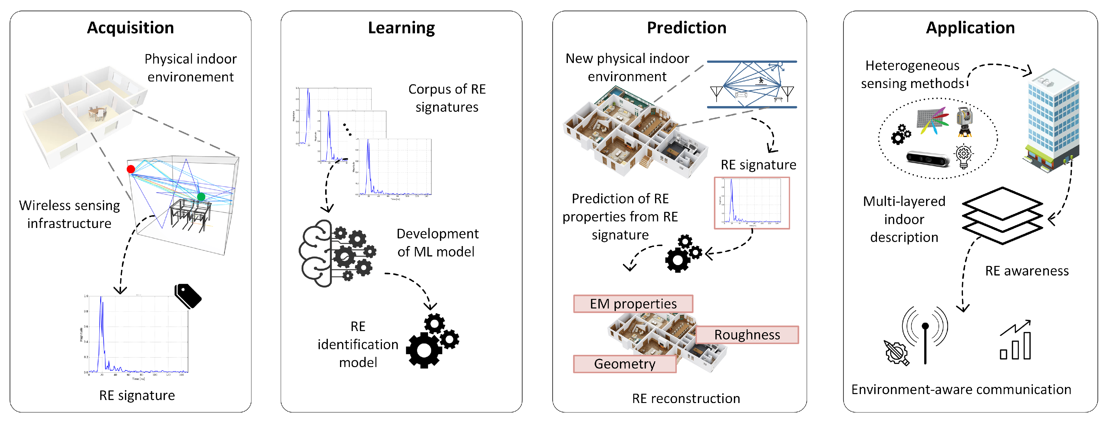
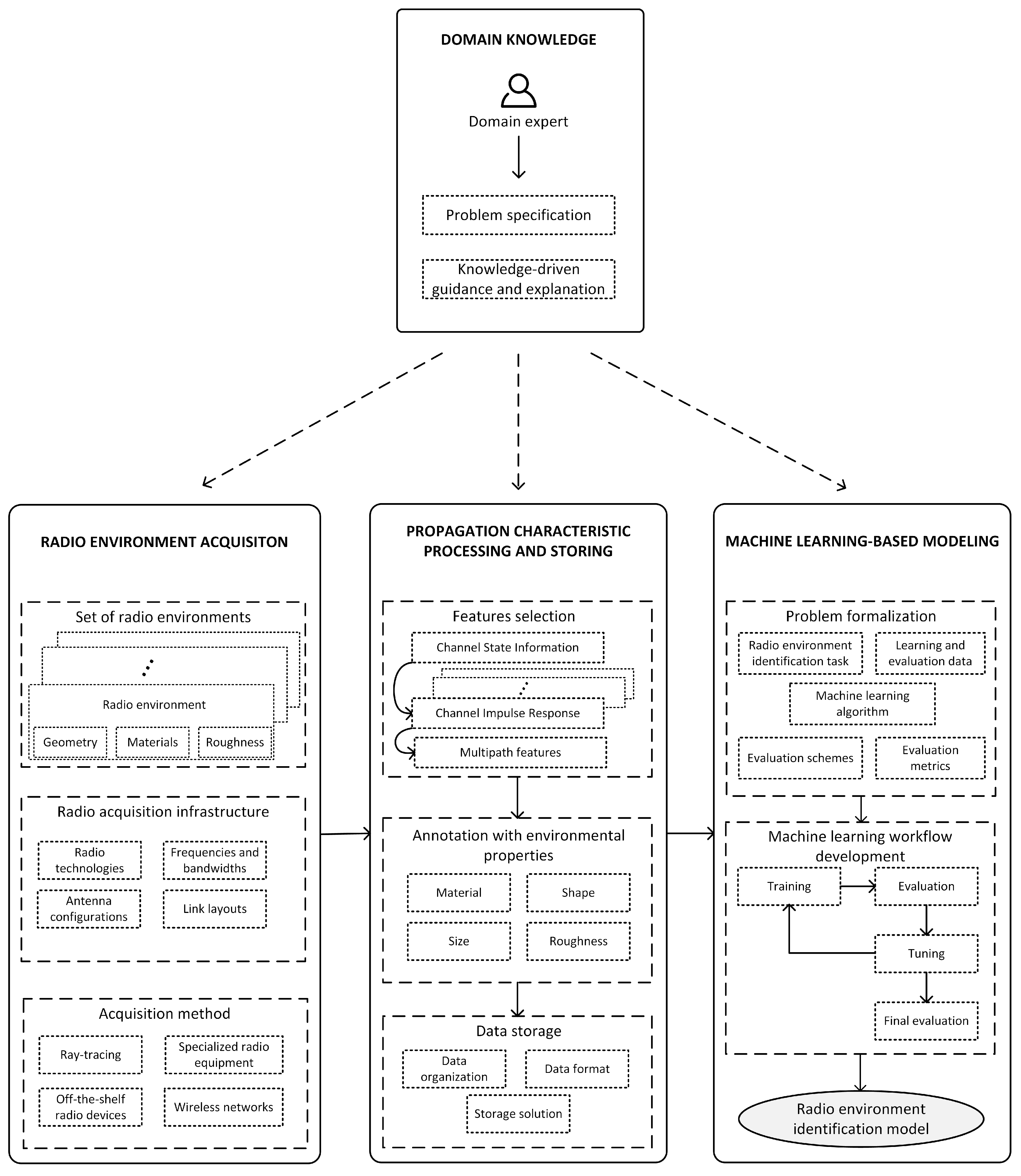
3. Intelligent Indoor Environment Characterization

To provide a comprehensive description of the indoor propagation environment using predictive models learned from RE signatures, we further extend the approach presented in our previous work [19]. The methodology for identifying the material of a single wall is modified to extend its application to the identification of several properties of the propagation environment that affect radio propagation, including (i) the materials of all facets, (ii) the size and shape of the room, and (iii) the roughness of the surfaces. The extended methodology provides an important environmental context for developing pioneering methods for improved indoor radio communications in the era of next-generation communications and for a detailed digital twin of indoor structures in future cities.

3.1. Concept

The methodology is based on two assumptions: (i) inside buildings, the received signal conveys a unique RE signature as a result of the interaction of the transmitted waves with the environment, and (ii) the CIR can be accurately estimated for a wireless link.
The key phases of the proposed approach, shown in Figure 1, are acquisition, learning, prediction, and application. A large corpus of RE signatures is a prerequisite for training RE identification models and validating their practical applicability. A large number of radio devices with sensing capabilities deployed indoors opens the possibility of using wireless infrastructure to capture RE signatures. It is assumed that a state-of-the-art machine learning algorithm can learn an RE identification model from the relationship between the RE signatures and the properties of the propagation environment. This study focuses on properties with discrete values and can be extended for continuous values. It is expected that the model can accurately predict the properties of a new indoor propagation environment for an input RE signature. The properties identified by the RE identification model could be incorporated into a multilayer description of the building that includes information about various aspects of the structure obtained using heterogeneous sensing methods. Improved RE awareness is seen as a necessary prerequisite for the development of novel methods for environmentally aware wireless communications.

3.2. Data-Driven Methodology

Indoor environment characterization is tackled using a data-driven methodology that eliminates the necessity for specialized scanning equipment. The methodology consists of four modules: (1) domain knowledge, (2) RE acquisition, (3) propagation characteristic processing and storing, and (4) machine-learning-based modeling. Figure 2 depicts the components of the methodology.
The incorporation of domain knowledge has a crucial role in the methodology, to ensure that the predictive model developed is relevant and useful for the intended application. The source of the knowledge is a radio communication expert with an in-depth understanding of indoor radio propagation and methods for estimating channel state information (CSI). Specifically, the domain expertise is used to select the indoor environments for training and evaluating the models, to choose an adequate method for the RE signature acquisition, to specify the meaningful features from the received signal that convey most of the environmental information, to formalize the learning task, to define the evaluation schemes, and to interpret the performance of the models.
The acquisition of RE signatures is of pivotal significance for the training and evaluation of the RE identification models. The collection of RE signatures involves (i) selecting a set of indoor environments, (ii) setting up the radio acquisition infrastructure, and (iii) selecting the acquisition method. Considering a large set of rooms with different sizes, materials, and roughness of the surfaces is important to obtain sufficient experience for the algorithms.
The setup of the radio acquisition infrastructure includes radio technology, carrier frequency and bandwidth, antenna type and configuration, and location of the radio nodes. Current and emerging technologies with wide bandwidth and fine time resolution needed for resolving the signal contributions arriving from different propagation paths can be used. To capture the unique signature of the environment for different radio node locations, the radios should be placed on a grid that covers the entire room. Individual or combined use of simulated and experimental methods, such as ray tracing, specialized radio equipment, off-the-shelf radio devices, and wireless networks, are appropriate for estimating propagation characteristics.
The raw propagation data is an input to the processing and storing module which includes (i) selecting CIR multipath features from CSI, (ii) annotating the formatted RE signatures with environmental properties, and (iii) storing the data in a format suitable for further machine learning analysis. The propagation characteristics of the MPCs, which convey most of the environmental information, are used as features. The environmental properties are categorical output labels, and a binary value is assigned to the input features of the RE signature to indicate the presence/absence of a property in the radio link surrounding. The RE signature is labeled with information about the properties of the indoor environment obtained from the model of the building or the building documentation. The data is organized in tabular form and stored in a comma-separated values (CSV) format compatible with a wide range of tools and libraries for machine learning analysis.
The machine-learning-based modeling module includes (i) the formalization of the problem and (ii) the development of the machine learning workflow. In the problem formalization step, the RE identification task is defined, the evaluation scheme and evaluation metrics are specified, and adequate data is selected from the available database for training, tuning, and final evaluation of the predictive model. The models are trained, evaluated, and tuned by adjusting the hyper-parameters. The optimal hyper-parameter values are found using a 5-fold cross-validation on the training set and an exhaustive search over all combinations of values in the defined search space. The predictive performance of the fine-tuned RE identification model is assessed on a separate test set that has not been used in the training and tuning phases.

4. Methodology Evaluation Procedure

The proposed methodology is applied to build predictive models for the identification of all materials in a plain room from CIR. The objective is to learn a predictive model based on the relation between CIR and the materials. A training set of CIRs associated with a binary indication of the presence/absence of materials in the room is used.

4.1. Learning Task Formalization

The task is formalized as a multi-label classification (MLC) task [83]. The main property of MLC is that each sample is annotated with multiple labels simultaneously. The goal is to learn a predictive model(s) that distinguishes relevant from irrelevant labels for a given data point. It is a reformulation of the binary classification task, where the goal is to predict multiple outputs simultaneously instead of one. MLC tasks can be formally defined as follows [84].
Given:
  • input space X , consisting of tuples of continuous values, where X i X , X i = ( x i 1 , x i 2 , , x i d ) is the input description of the sample i and D is the size of the tuple, i.e., the number of input attributes;
  • label space L = { l 1 , l 2 , , l L } , which is a set of possible discrete labels, where L = | L | and L > 1 ;
  • training set D = { ( X i , Y i ) | X i X , Y i L , 1 i N } , where ( X i , Y i ) is a multi-labeled training sample and N = | D | is the number of samples in the training set;
  • a quality criterion q, which rewards models with good predictive performance and low complexity.
Find: a function h, such that h: X 2 L while optimizing q.
The CIR of a wireless link is considered as the input description of the data sample associated with the particular link. Three propagation characteristics are considered as input features describing the i-th MPC: received power P i , phase shift Φ i and time of arrival τ i . The i-th input sample is X i = ( P i , 1 , Φ i , 1 , τ i , 1 , , P i , R , Φ i , R , τ i , R ) , where R is the number of propagation paths reaching the receiver. The number of input variables considered in the experiments is 45 ( D = 45 ), for three MPC characteristics of the 15 strongest MPCs ( R = 15 ) resolved at the receiver site, considering UWB technology with power above the receiver sensitivity set to −250 dBm, including the direct component and the first- and second-order reflected components. In cases where the number of MPCs above the receiver sensitivity is lower than 15, all of the meaningful components should be considered. The training set contains CIRs labeled with the materials of the surfaces in the room. The label space is L = { b r i c k ,   c o n c r e t e ,   g l a s s ,   p l a s t e r ,   w o o d } and L = 5 . The number of samples is equal to the product of the number of rooms and the number of radio links.

4.2. Learning Approach

The learning task is approached with a problem transformation method [83]. The method transforms the task into multiple single-target classification tasks that share the input space, and applies binary classification algorithms to learn individual predictive models for each label. In the prediction phase, all binary classifiers are invoked and their individual predictions are merged to obtain the final prediction. Four different learning algorithms are considered: decision tree (DT) [85], random forest (RF) [86], support vector machine (SVM) [87], and multilayer perceptron (MLP) [88], as representatives of tree-based algorithms, ensemble algorithms, kernel-based algorithms, and neural networks, respectively.
The DT algorithm constructs tree-like models with a hierarchical structure. A classifier tree is built using a tree-construction algorithm, known as top-down induction of DTs (TDIDT) [89]. The TDIDT uses a divide-and-conquer approach for recursively growing trees, starting at the root node and descending to the leaves. A univariate splitting criterion is used. The learner uses the information gain or gini index of diversity [90] to find the attribute at which to perform the split. Pre-pruning is considered to prevent fully grown trees and overfitting.
The RF algorithm is used to create multiple independent tree models and integrate the individual predictions into a final prediction. In this study, the ensemble prediction is created by averaging the probabilistic prediction of the individual models. Each tree of the ensemble is constructed using a bootstrap sample of the training set [91]. During the construction of the tree, the best split is found from a random subset of the input features. The individual trees are pruned beforehand.
The SVM algorithm constructs a separating hyperplane in a high-dimensional feature space that results in maximum separation between classes. If the classes are not linearly separable in the original space, a kernel function is used to map the data in the higher-dimensional space where linear boundaries exist. The selection of an adequate kernel function and a value for the regularization parameter is essential for building an optimal SVM model.
The MLP is a feed-forward neural network [92] that consists of artificial neurons that compute the weighted inputs and apply a nonlinear activation function [93] to produce an output. Training of the network includes feed-forward, cost computation, back-propagation, and weight update.
Implementations of the algorithms from the Scikit-learn Python library are used [94,95]. The literature confirms the reliability of the implementations in various application domains [96]. The hyper-parameters with the most significant impact on the performance of the models are tuned using the grid-search method. The values of the hyper-parameters included in the search space are given in Table 1.

4.3. CIR Acquisition

Data for training and evaluation of the models is collected using the ray-tracing method [97] assuming an ultra-wideband (UWB) system [98] with a fine time resolution needed for distinguishing the MPCs [99] and a microwave frequency band [100]. The data that we generated is annotated with labels describing the location of the radio nodes, the geometry of the room, and the material of the surfaces [101]. The data set can also be used for other studies that require indoor propagation data.
We consider 3750 room types in terms of the surface materials in three sizes: small (3 m × 3 m), medium (5 m × 5 m), and large (7 m × 7 m), referred to as S, M, and L, respectively, for a total of 11,250 rooms. Six smooth facets bound the rooms, the height between the floor and ceiling is 3 m, and the rooms are plain (i.e., without interacting objects). The materials used for the facets in the rooms are shown schematically in Figure 3. The floors are built of concrete or wood, the ceilings are built of concrete, plaster, or wood, and the walls are built of brick, concrete, glass, plaster, or wood. The number of different room types is derived from the materials used for the floors and ceilings, where there are six floor–ceiling material combinations, and the materials used for walls, which have 625 material combinations. The materials are defined with the relative permittivity and conductivity [102].
Spatially distributed CIRs are acquired with radio nodes placed in fixed locations of a predefined topology and a portable node moved over a uniform grid covering the room. The positioning of fixed nodes shown in Figure 4 is defined by the following three topologies:
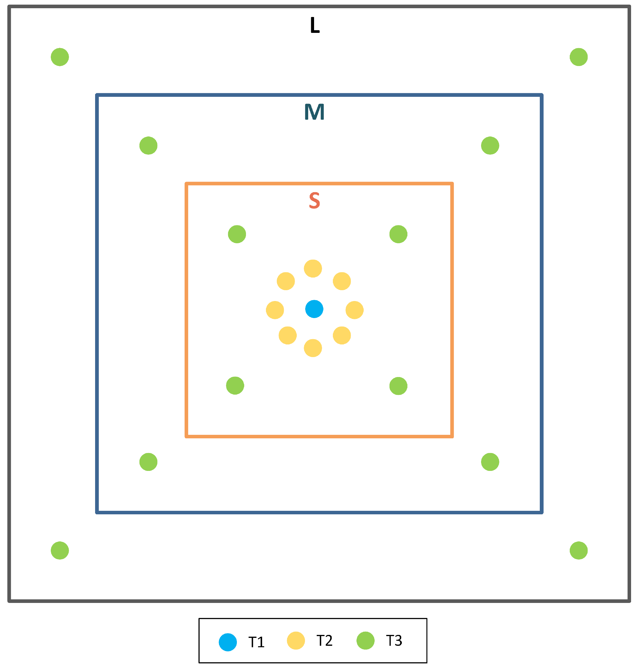
  • Center (T1): a single radio node in the center of the room;
  • Circle (T2): eight radio nodes spaced π / 4 rad apart on a circle with radius 0.5 m;
  • Corners (T3): four radio nodes located 0.375 m from the walls, near the corners of the room.
The topologies are defined to correspond to the most common practices for the wireless systems in operation: (i) central placement of the node with single or multiple antennas arranged on a circle, and (ii) access points or base stations near the corners of the room. The grid indicates the possible positions of the portable node. The grid covers the room with grid lines spaced 0.25 m apart, resulting in a total of 121, 361, and 729 grid positions in S, M, and L rooms, respectively. To ensure that the data sets include CIRs from nodes distributed throughout the room, one grid position is randomly selected from each 1 m × 1 m region for training and testing.
The links between the fixed nodes in the T1, T2, and T3 topologies and the portable node at the selected positions (9 positions in S rooms, 25 positions in M rooms, and 49 positions in L rooms) used for collecting the training and test data are referred to as L1-train and L1-test, L2-train and L2-test, and L3-train and L3-test, respectively. The number of radio links between the fixed nodes in the different topologies and the portable node moved across the selected grid positions for training and testing in the different room sizes is summarized in Table 2.
Omnidirectional antennas are used, mounted 1.5 m above the floor. The carrier frequency is equal to 3494.4 MHz, and the bandwidth is 466.2 MHz. The input power is set to 0 dBm and the polarization is vertical. A commercially available 3D wireless prediction software, Remcom Wireless InSite [103], is used, which is capable of adequately estimating the effects of buildings on the propagation of electromagnetic waves and generating accurate values for specific propagation characteristics [104]. A three-dimensional propagation model and a shooting and bouncing ray-tracing method with exact path correction are used [105].

4.4. Evaluation Scenarios

One of the most important aspects of ML-based modeling is the choice of the evaluation scenario that determines the selection of data used in the training and testing phases. The room sizes and radio links included in the training procedure can affect the generality of the models and their ability to make correct predictions to new data, and thus the applicability to different use cases. To investigate the performance of the models in several realistic use cases, we defined three scenarios that differ in the room sizes where the CIRs are acquired for training and testing and in the positioning of the radio nodes. The scenarios are defined as follows:
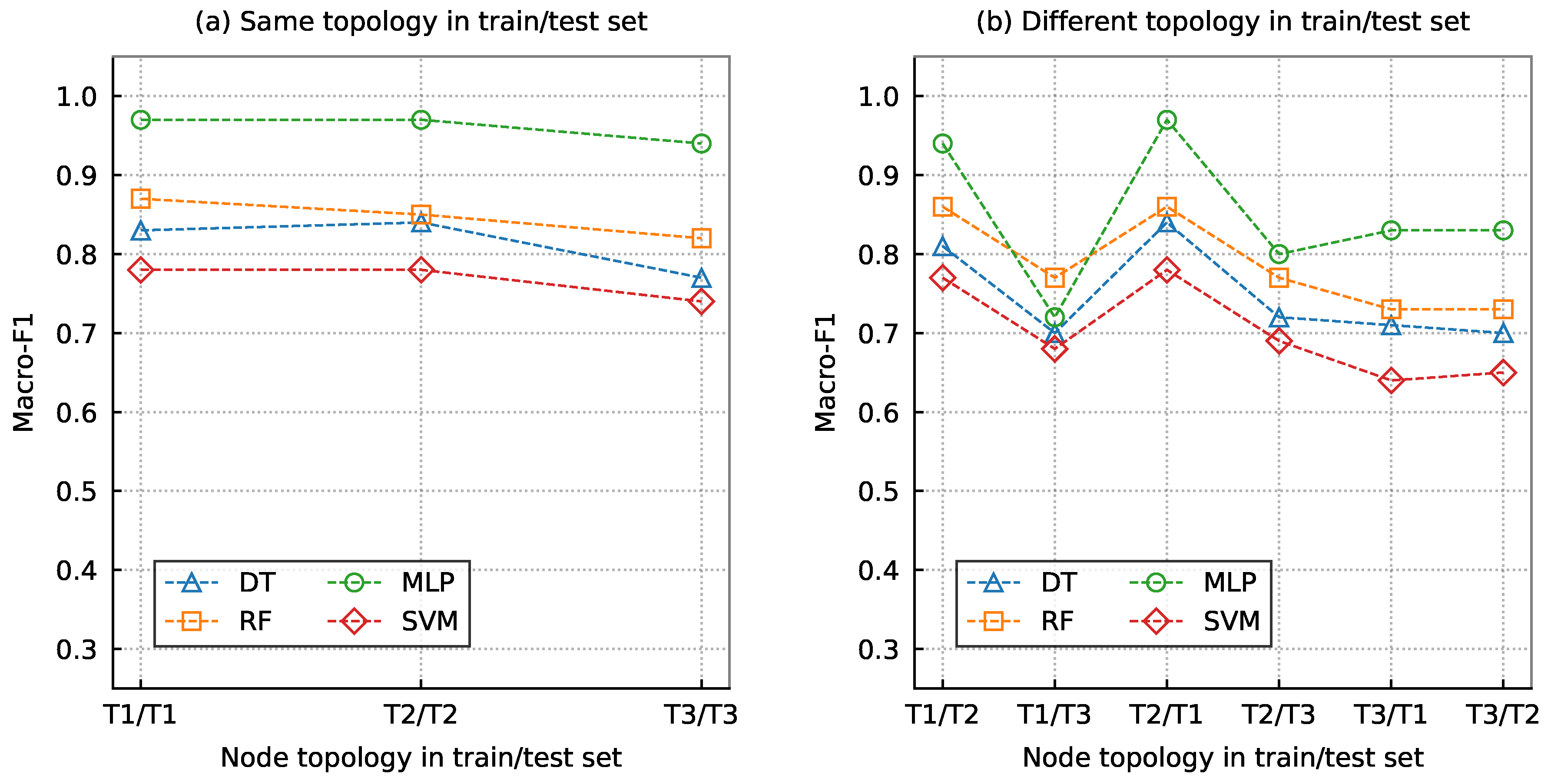
  • Scenario Init: Represents the case where the models are applied to CIR data from rooms with sizes considered in the training procedure. The same and different locations of the fixed nodes are used to estimate the CIRs for training and testing;
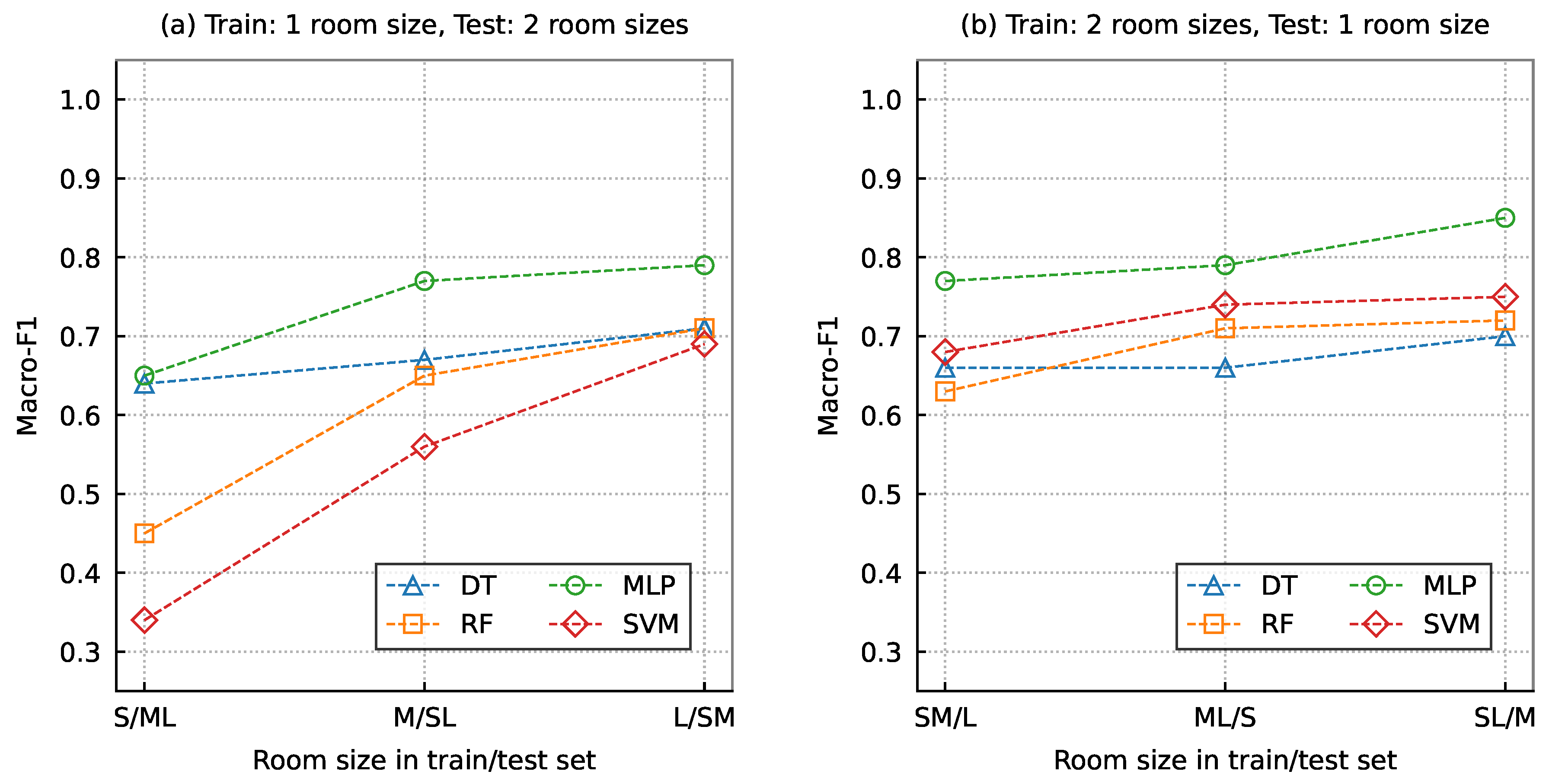
  • Scenario Diff-RS: Represents the case where the models are applied to CIR data from rooms with sizes that were not considered in the training procedure. The same locations of the fixed nodes that were used for estimating the CIRs for training are used for testing;
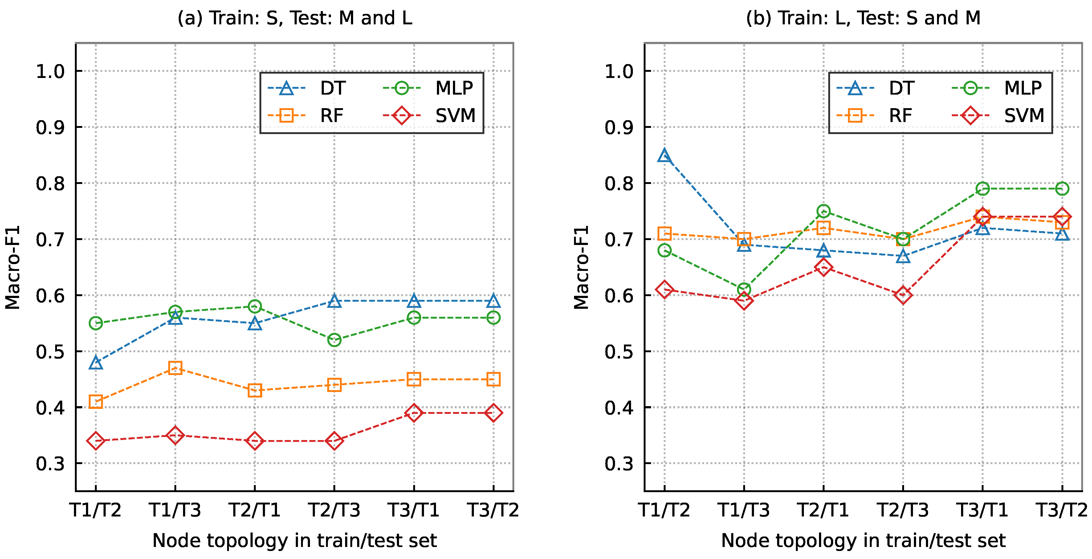
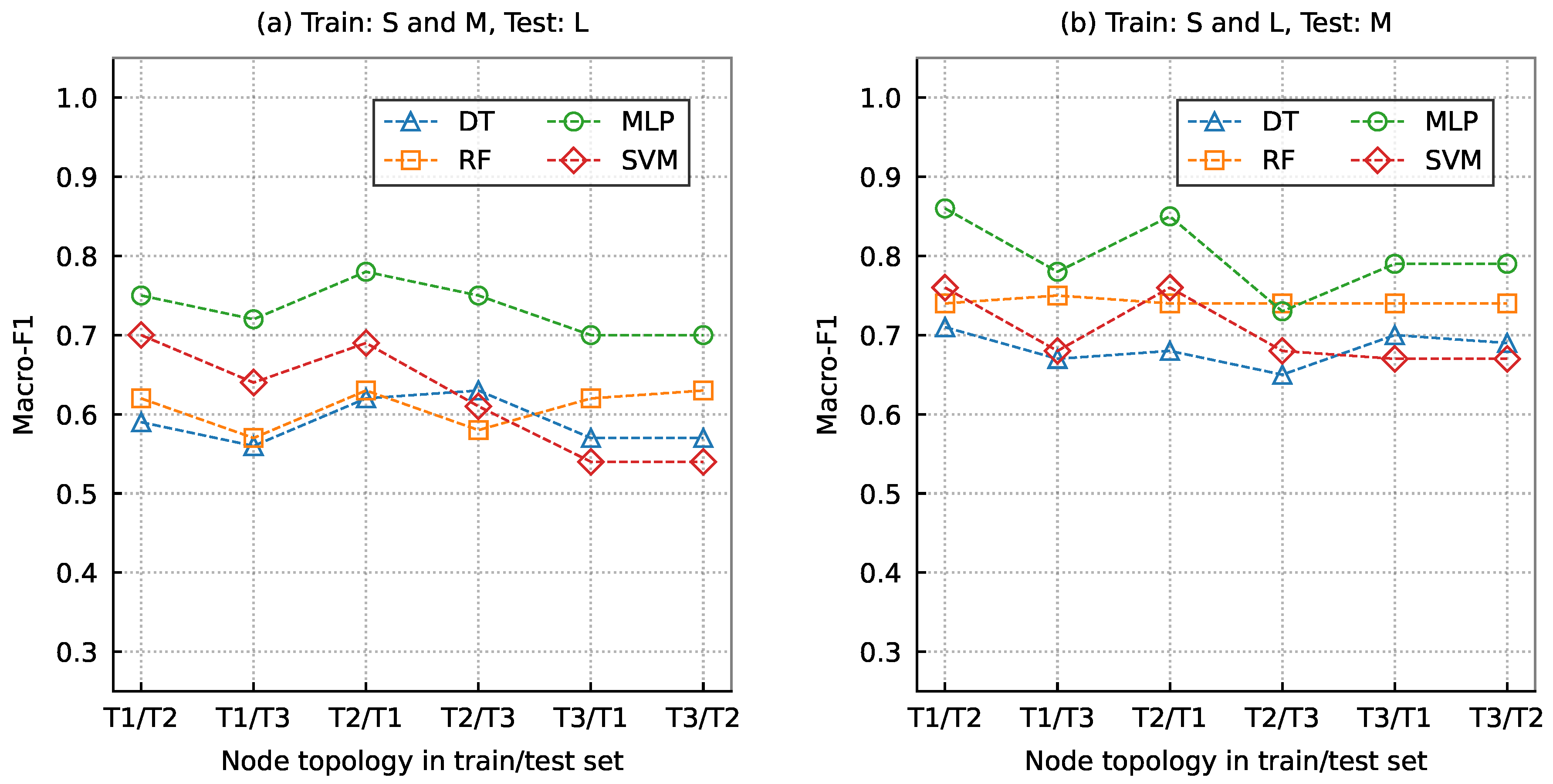
  • Scenario Diff-RS-Lyt: Represents the case where the models are applied to CIR data from different radio links in rooms with sizes that were not considered in the training procedure. Different locations of the fixed nodes are used for estimating the CIRs for training and testing.
In all scenarios, the portable node is moved to different locations to estimate CIRs for training and testing over the grid, as described in Section 4.3. The room sizes and node topologies included in the training and test sets for the different scenarios are summarized in Table 3.
The scenario Init represents an initial case where data are available in the training phase from all room sizes to which the model is to be applied. In more advanced use cases, including data from all room sizes and link locations in the training set may be unfeasible if the range of room sizes is large, some room sizes are rare, CIR estimation is expensive, or CIR estimates from some link locations are not available. Thus, in scenario Diff-RS and scenario Diff-RS-Lyt, the performances of models trained with data from a single room size and models trained with data from two room sizes are assessed when applied to a room with different sizes. The impact of merging data from two room sizes and the impact of the room size used for testing relative to the room sizes used for training is studied.
To quantitatively measure the performance of models in predicting outcomes, the F1 score is used [83,90]. It is the harmonic mean of precision and recall. In the case of MLC, the F1 score represents the per-label metric calculated based on the true positives (TP), true negatives (TN), false positives (FP), and false negatives (FN) as
F 1 = 2 p r e c i s i o n 1 + r e c a l l 1 = 2 T P 2 T P + F P + F N .
The macro-averaged F1 score is calculated as the unweighted mean of the metric across all labels. We adhere to the approaches recommended in [106] for calculating the metric. In this work, the models with a predictive performance in terms of the F1 score above 0.5 are considered usable, i.e., applicable for the material identification task. Higher values of the F1 score indicate better predictive performance. In the future, the threshold for acceptable model performance will be specified with the requirements of the use cases.

5. Results and Discussion

We examined the impact of the room sizes and positioning of the radio nodes used in the training phase on the ability of the predictive models to accurately identify the materials in the different scenarios.
The identification of materials in rooms that are the same size as the rooms used to obtain the training data is discussed based on the results of the scenario Init, presented in Figure 5. The results confirm the applicability of the models to rooms with sizes considered in the training phase. The high predictive performance of the models is achieved due to the following: (i) a strong relation exists between CIR and the surface materials in a room due to the reflection coefficient’s dependence on the materials’ EM properties, and (ii) the same room sizes were used in the training and testing phases.
In the basic case, where the positioning of the fixed nodes in the testing phase is the same as in the training phase, the models have F 1 scores above 0.7. From Figure 5a, it can be seen that when data from radio links with fixed nodes in topology T3 are used for training and testing, the models have slightly lower performance than when topology T1 or T2 is used. This is due to the location of the fixed nodes relative to the walls: the fixed nodes in topologies T1 and T2 are placed centrally in the room and have approximately the same distance to all walls, while the fixed nodes in topology T3 are placed near the corners and the distance to some walls is smaller than to others. Namely, when the fixed nodes are not placed symmetrically with respect to the room geometry, they are closer to some walls and the information about the material loaded in CIR is richer; thus, the models can identify the material of these walls more accurately.
In the case where different topologies of the fixed nodes are used in the training and testing phases, the ability of the model to accurately identify the materials is affected by the distance between the nodes used and their position relative to the room geometry, as shown in Figure 5b. Due to the similar location (central) of the nodes in topologies T1 and T2, the models trained with data from one of the topologies make predictions on data from the other topology with similar performance as when making predictions on data from the same topology that is used for training. A drop in performance is observed when the models are tested with data from topology T3. The models trained with data from topology T3 have similar performance when making predictions using data from T1 or T2.
The results show that the identification of the materials is possible when the CIRs are estimated with fixed nodes at locations that were not considered when training the models. The change in the location of the fixed node used for training and testing is small, resulting in a change in the CIR that is not significant, and thus the models can correctly predict the materials from the CIRs included in the test set. This finding confirms that the proposed approach is promising in scenarios where the locations of the fixed nodes used in the training phase are not known or the nodes cannot be placed at the same locations in the environment that has to be characterized. Due to the different amounts of environmental information in the CIRs and the slight change in the CIR estimated with different radio links, the identification is slightly less accurate when the locations of the fixed nodes are not included in the training process.
The ability of the models to make accurate predictions when applied in rooms with sizes that were not considered in the training phase using locations of the fixed node that were included in the training set is analyzed using the results of the scenario Diff-RS, shown in Figure 6. These results confirm that most of the models can be applied in scenarios where the size of the room being characterized was not represented in the training process. The use of CIRs from radio links covering the room for training the models, and thus considering the RE signatures from CIRs uniformly distributed over the room, explains the predictive performance of the models.
The size of the room being characterized relative to the size of the rooms used to train the model affects the predictive performance of the models. From Figure 6a, it is evident that the models trained with the MLP or DT algorithms are usable for the task even when the size of the rooms used for training the model are smaller than the size of the room in which the model is applied (train: S, test: M and L). Training the models with data from rooms that are larger compared to the rooms where the models are applied (train: L, test: S and M) results in better identification of the materials. Using larger rooms in the training phase results in models with wider practical applicability due to a large number of positions of the portable node and, thus, a large number of radio links. A large number of links in the training phase means that the algorithm can learn from a large corpus of spatially diverse RE signatures. Furthermore, the model in the large rooms learns also the propagation path-loss, while in small rooms the paths are much shorter, thus the path-loss is not so significant.
According to the results shown in Figure 6b, the models trained with data from rooms with two room sizes can accurately identify the materials in larger rooms, smaller rooms, and rooms whose sizes are between the sizes of the rooms used for training. When the models are applied to larger rooms (train: S and M, test: L), the prediction performance is slightly lower compared to the other two cases (train: M and L, test: S or train: S and L, test: M). The room sizes that need to be included in the training set should be determined according to the size of the rooms where the model will be used. In scenarios where the intended use of the model is not specified before training, including many room sizes in the training set—selected according to the most common sizes in office and residential buildings—can result in accurate models with good predictive capabilities.
The results of scenario Diff-RS-LYT for the case where a single room size is used to train the models are shown in Figure 7. Applying the models to CIRs estimated with a fixed-node topology, which was not considered in the acquisition of the training CIRs, highlights the impact of the room size used for training the models on their capability to make accurate predictions. The models trained with data from rooms larger than the rooms in which they are applied (train: L, test: S and M) have better F 1 scores than the models trained with data from smaller rooms (train: S, test: M and L).
When data from L rooms is used for training, different algorithms lead to the best models for different topologies of fixed nodes used to collect the training and testing data. With a training set estimated with topology T1, the algorithms DT and RF learn the models with the best performance when tested with data from topologies T2 or T3. The models learned with the MLP and RF algorithms with training data estimated with topology T2 perform best when tested with data from topologies T1 or T3. The models learned with the MLP algorithm on the training data from topology T3 have the highest F 1 scores when tested with data from topologies T1 or T2.
The performance of the models trained with data from two room sizes in scenario Diff-RS-LYT are shown in Figure 8. These results confirm the conclusions drawn for scenario Diff-RS for the case where the fixed-node topology used in the train and test phases is different. In particular, training with data from smaller and larger rooms compared to the size of the rooms where the model is applied (train: S and L, test: M) leads to better performance than training with data from smaller rooms compared to the size of the rooms where the model is applied (train: S and M, test: L), which is due to the path-loss information included in the training phase.
Analysis of the predictive performance of the models confirmed that the materials of the surfaces can be accurately identified. The models are able to accurately identify the materials in rooms with new sizes from CIRs estimated with different topologies of fixed nodes. In most evaluation scenarios, the MLP models show superior performance. In most cases, the tree-based models show slightly lower performance. Ensembles of trees tend to score higher than single-tree models, reflecting the advantages of combining multiple trees. SVM models show the lowest performance and sensitivity to the fixed-node topology used for CIR estimation.

6. Conclusions and Future Work

This paper presents the methodology and performance evaluation of a CIR-based identification of all materials used for surfaces in an indoor environment. The proposed methodology has great potential in environmentally aware wireless communications. It can also be useful for enriching the digital twin of the room with information about the materials used for the surfaces.
The problem of material identification is investigated using machine learning approaches. The locations of the radio nodes for CIR acquisition were specified. A large amount of UWB data was collected for numerous rooms built of different materials and models were developed using the DT, RF, MLP, and SVM algorithms. Different evaluation scenarios were defined to assess the predictive performance of the models, to evaluate the applicability of the proposed method to different realistic use cases, and to investigate how the radio node locations and room sizes affect the generality of the models and the material identification. The results confirm that the materials of all surfaces in a room can be accurately identified using RE identification models. The MLP models have the best performance on most test sets. It is shown that the proposed method can be generalized to different scenarios defined in terms of the location of the radio nodes and the sizes of the rooms and the trained models are applicable for the identification of the materials based on CIR from rooms and radio links that were not used during the training process. However, using the same locations of the fixed nodes as in the training phase results in a more accurate identification of the materials.
The presented work can be extended to comprehensively explore the potential of the proposed approach and its accuracy, applicability, and usefulness for various system configurations in environments with a mixture of materials and interacting objects becoming relevant as the frequency increases. Building on the presented findings, future work will focus on (1) leveraging cutting-edge machine learning approaches to model the relation between the RE signature and the indoor RE properties, and (2) exploiting the potential of state-of-the-art approaches from wireless communications. In particular, a higher-frequency band with larger bandwidth, leading to better time resolution of CIR, and multiple antenna systems that allow accurate estimation of the angle of arrival, will be utilized. This would provide a more accurate estimation of the RE signature, allowing the approach to be extended to characterize surfaces with multiple materials in realistic environments with many scatters. Due to the lack of publicly available indoor propagation data, further data collection campaigns are needed to validate the models in real indoor environments and for different configurations of the wireless system. We started an extensive CIR measurement campaign in versatile indoor environments by UWB transceivers compliant with the IEEE 802.15.4-2011 standard and antenna arrays for angle of arrival estimation.

Author Contributions

Conceptualization, T.K., T.J., A.Š., A.R. and A.H.; methodology, T.J., A.Š. and A.H.; software, T.K.; validation, T.J., A.Š. and A.H.; formal analysis, T.K.; investigation, T.K. and A.R.; resources, T.K.; data curation, T.K.; writing—original draft preparation, T.K.; writing—review and editing, T.J., A.Š., A.R. and A.H.; visualization, T.K., T.J., A.R. and A.H.; supervision, A.R. and A.H.; project administration, A.Š.; funding acquisition, A.Š. All authors have read and agreed to the published version of the manuscript.

Funding

This research was funded by the Slovenian Research Agency (Grant nos. P2-0016, J2-2507, and P2-0095).

Data Availability Statement

The data collected for the analysis presented in this study are openly available in the repository Zenodo [101].

Acknowledgments

T.K. acknowledges the Ad-Futura scholarship for doctoral studies awarded by the Public Scholarship, Development, Disability, and Maintenance Fund of the Republic of Slovenia.

Conflicts of Interest

The authors declare no conflict of interest.

Abbreviations

  • The following abbreviations are used in this manuscript:
    AllCenter+Circle+Corners
    All/AllTrain: Center+Circle+Corners, test: Center+Circle+Corners
    CIRChannel impulse response
    CSVComma-separated-values
    DTDecision tree
    FNFalse negatives
    FPFalse positives
    LLarge
    LoSLine-of-sight
    L/SMTrain: large, test: small+medium
    L1-testLinks with a fixed node in topology Center for testing
    L1-trainLinks with a fixed node in topology Center for training
    L2-testLinks with a fixed node in topology Circle for testing
    L2-trainLinks with a fixed node in topology Circle for training
    L3-testLinks with fixed nodes in topology Corners for testing
    L3-trainLinks with fixed nodes in topology Corners for training
    MMedium
    M/SLTrain: medium, test: small+large
    MLMedium+large
    ML/STrain: medium+large, test: small
    MLCMulti-label classification
    MLPMultilayer perceptron
    MPCMultipath component
    NLoSNon-line-of-sight
    RFRandom forest
    RGBRed–green–blue
    SSmall
    S/MLTrain: small, test: medium+large
    SLSmall+large
    SL/MTrain: small+large, test: medium
    SLAMSimultaneous localization and mapping
    SMSmall+medium
    SM/LTrain: small+medium, test: large
    SML/SMLTrain: small+medium+large, test: small+medium+large
    SVMSupport vector machine
    T1Fixed-node topology Center
    T1/T1Train: Center, test: Center
    T1/T2Train: Center, test: Circle
    T1/T3Train: Center, test: Corners
    T2Fixed-node topology Circle
    T2/T1Train: Circle, test: Center
    T2/T2Train: Circle, test: Circle
    T2/T3Train: Circle, test: Corners
    T3Fixed-node topology Corners
    T3/T1Train: Corners, test: Center
    T3/T2Train: Corners, test: Circle
    T3/T3Train: Corners, test: Corners
    TNTrue negatives
    TPTrue positives
    UWBUltra-wideband

References

  1. Saad, W.; Bennis, M.; Chen, M. A Vision of 6G Wireless Systems: Applications, Trends, Technologies, and Open Research Problems. IEEE Netw. 2020, 34, 134–142. [Google Scholar] [CrossRef] [Green Version]
  2. Zeng, Y.; Xu, X. Toward Environment-Aware 6G Communications via Channel Knowledge Map. IEEE Wirel. Commun. 2021, 28, 84–91. [Google Scholar] [CrossRef]
  3. Deren, L.; Wenbo, Y.; Zhenfeng, S. Smart city based on digital twins. Comput. Urban Sci. 2021, 1, 1–11. [Google Scholar] [CrossRef]
  4. Jiang, W.; Han, B.; Habibi, M.A.; Schotten, H.D. The Road Towards 6G: A Comprehensive Survey. IEEE Open J. Commun. Soc. 2021, 2, 334–366. [Google Scholar] [CrossRef]
  5. El-Sheimy, N.; Li, Y. Indoor navigation: State of the art and future trends. Satell. Navig. 2021, 2, 1–23. [Google Scholar] [CrossRef]
  6. Gu, F.; Hu, X.; Ramezani, M.; Acharya, D.; Khoshelham, K.; Valaee, S.; Shang, J. Indoor Localization Improved by Spatial Context—A Survey. ACM Comput. Surv. 2019, 52, 1–35. [Google Scholar] [CrossRef] [Green Version]
  7. Tseng, P.Y.; Lin, J.J.; Chan, Y.C.; Chen, A.Y. Real-time indoor localization with visual SLAM for in-building emergency response. Autom. Constr. 2022, 140, 104319. [Google Scholar] [CrossRef]
  8. Vijayan, D.; Rose, A.L.; Arvindan, S.; Revathy, J.; Amuthadevi, C. Automation systems in smart buildings: A review. J. Ambient. Intell. Humaniz. Comput. 2020, 1–13. [Google Scholar] [CrossRef]
  9. Pintore, G.; Mura, C.; Ganovelli, F.; Fuentes-Perez, L.; Pajarola, R.; Gobbetti, E. State-of-the-art in Automatic 3D Reconstruction of Structured Indoor Environments. Comput. Graph. Forum 2020, 39, 667–699. [Google Scholar] [CrossRef]
  10. Huang, C.; He, R.; Ai, B.; Molisch, A.F.; Lau, B.K.; Haneda, K.; Liu, B.; Wang, C.X.; Yang, M.; Oestges, C.; et al. Artificial Intelligence Enabled Radio Propagation for Communications—Part II: Scenario Identification and Channel Modeling. IEEE Trans. Antennas Propag. 2022, 70, 3955–3969. [Google Scholar] [CrossRef]
  11. Sun, Y.; Peng, M.; Zhou, Y.; Huang, Y.; Mao, S. Application of Machine Learning in Wireless Networks: Key Techniques and Open Issues. IEEE Commun. Surv. Tutor. 2019, 21, 3072–3108. [Google Scholar] [CrossRef] [Green Version]
  12. Liu, F.; Cui, Y.; Masouros, C.; Xu, J.; Han, T.X.; Eldar, Y.C.; Buzzi, S. Integrated Sensing and Communications: Toward Dual-Functional Wireless Networks for 6G and Beyond. IEEE J. Sel. Areas Commun. 2022, 40, 1728–1767. [Google Scholar] [CrossRef]
  13. Nie, G.; Zhang, J.; Zhang, Y.; Yu, L.; Zhang, Z.; Sun, Y.; Tian, L.; Wang, Q.; Xia, L. A predictive 6G network with environment sensing enhancement: From radio wave propagation perspective. China Commun. 2022, 19, 105–122. [Google Scholar] [CrossRef]
  14. Zhang, J.; Liu, L.; Fan, Y.; Zhuang, L.; Zhou, T.; Piao, Z. Wireless Channel Propagation Scenarios Identification: A Perspective of Machine Learning. IEEE Access 2020, 8, 47797–47806. [Google Scholar] [CrossRef]
  15. Seretis, A.; Sarris, C.D. An Overview of Machine Learning Techniques for Radiowave Propagation Modeling. IEEE Trans. Antennas Propag. 2022, 70, 3970–3985. [Google Scholar] [CrossRef]
  16. Sarker, I.H. Machine learning: Algorithms, real-world applications and research directions. SN Comput. Sci. 2021, 2, 160. [Google Scholar] [CrossRef] [PubMed]
  17. Gündüz, D.; de Kerret, P.; Sidiropoulos, N.D.; Gesbert, D.; Murthy, C.R.; van der Schaar, M. Machine Learning in the Air. IEEE J. Sel. Areas Commun. 2019, 37, 2184–2199. [Google Scholar] [CrossRef] [Green Version]
  18. Hrovat, A.; Guam, K.; Kocevska, T.; Javornik, T. 3D Indoor Environment Charactirazation based on Radio Scanning: Initial Idea and Methodolgy. In Proceedings of the 2019 23rd International Conference on Applied Electromagnetics and Communications (ICECOM2019), Dubrovnik, Croatia, 30 September–2 October 2019; pp. 1–6. [Google Scholar]
  19. Kocevska, T.; Javornik, T.; Švigelj, A.; Hrovat, A. Framework for the Machine Learning Based Wireless Sensing of the Electromagnetic Properties of Indoor Materials. Electronics 2021, 10, 2843. [Google Scholar] [CrossRef]
  20. Kocevska, T.; Javornik, T.; Švigelj, A.; Guan, K.; Rashkovska, A.; Hrovat, A. Comparison of Machine Learning Models for Predicting Indoor Materials from Channel Impulse Response. In Proceedings of the 2022 International Conference on Software, Telecommunications and Computer Networks (SoftCOM2022), Split, Croatia, 22–24 September 2022; pp. 1–6. [Google Scholar]
  21. AlHajri, M.I.; Ali, N.T.; Shubair, R.M. A Machine Learning Approach for the Classification of Indoor Environments Using RF Signatures. In Proceedings of the 2018 IEEE Global Conference on Signal and Information Processing (GlobalSIP2018), Anaheim, CA, USA, 26–29 November 2018; pp. 1060–1062. [Google Scholar]
  22. AlHajri, M.I.; Ali, N.T.; Shubair, R.M. Classification of Indoor Environments for IoT Applications: A Machine Learning Approach. IEEE Antennas Wirel. Propag. Lett. 2018, 17, 2164–2168. [Google Scholar] [CrossRef]
  23. Kaatze, U. Measuring the dielectric properties of materials. Ninety-year development from low-frequency techniques to broadband spectroscopy and high-frequency imaging. Meas. Sci. Technol. 2012, 24, 012005. [Google Scholar] [CrossRef]
  24. Landron, O.; Feuerstein, M.; Rappaport, T. In situ microwave reflection coefficient measurements for smooth and rough exterior wall surfaces. In Proceedings of the IEEE 43rd Vehicular Technology Conference, Secaucus, NJ, USA, 18–20 May 1993; pp. 77–80. [Google Scholar]
  25. Ahmadi-Shokouh, J.; Noghanian, S.; Keshavarz, H. Reflection Coefficient Measurement for North American House Flooring at 57–64 GHz. IEEE Antennas Wirel. Propag. Lett. 2011, 10, 1321–1324. [Google Scholar] [CrossRef]
  26. Lu, J.; Steinbach, D.; Cabrol, P.; Pietraski, P.; Pragada, R.V. Propagation characterization of an office building in the 60 GHz band. In Proceedings of the The 8th European Conference on Antennas and Propagation (EuCAP2014), The Hague, The Netherlands, 6–11 April 2014; pp. 809–813. [Google Scholar]
  27. Virk, U.T.; Nguyen, S.L.H.; Haneda, K.; Wagen, J.F. On-Site Permittivity Estimation at 60 GHz Through Reflecting Surface Identification in the Point Cloud. IEEE Trans. Antennas Propag. 2018, 66, 3599–3609. [Google Scholar] [CrossRef] [Green Version]
  28. Long, Y.; Zeng, Y.; Xu, X.; Huang, Y. Environment-Aware Wireless Localization Enabled by Channel Knowledge Map. In Proceedings of the GLOBECOM 2022—2022 IEEE Global Communications Conference, Rio de Janeiro, Brazil, 4–8 December 2022; pp. 5354–5359. [Google Scholar]
  29. Li, K.; Li, P.; Zeng, Y.; Xu, J. Channel Knowledge Map for Environment-Aware Communications: EM Algorithm for Map Construction. In Proceedings of the 2022 IEEE Wireless Communications and Networking Conference (WCNC), Austin, TX, USA, 10–13 April 2022; pp. 1659–1664. [Google Scholar]
  30. Wu, D.; Zeng, Y.; Jin, S.; Zhang, R. Environment-Aware and Training-Free Beam Alignment for mmWave Massive MIMO via Channel Knowledge Map. In Proceedings of the 2021 IEEE International Conference on Communications Workshops (ICC Workshops), Montreal, QC, Canada, 14–23 June 2021; pp. 1–7. [Google Scholar]
  31. Liu, M.; Fang, S.; Dong, H.; Xu, C. Review of digital twin about concepts, technologies, and industrial applications. J. Manuf. Syst. 2021, 58, 346–361. [Google Scholar] [CrossRef]
  32. Mylonas, G.; Kalogeras, A.; Kalogeras, G.; Anagnostopoulos, C.; Alexakos, C.; Muñoz, L. Digital Twins From Smart Manufacturing to Smart Cities: A Survey. IEEE Access 2021, 9, 143222–143249. [Google Scholar] [CrossRef]
  33. Dembski, F.; Wössner, U.; Letzgus, M.; Ruddat, M.; Yamu, C. Urban Digital Twins for Smart Cities and Citizens: The Case Study of Herrenberg, Germany. Sustainability 2020, 12, 2307. [Google Scholar] [CrossRef] [Green Version]
  34. Zlatanova, S.; Sithole, G.; Nakagawa, M.; Zhu, Q. Problems In Indoor Mapping and Modelling. Int. Arch. Photogramm. Remote Sens. Spat. Inf. Sci. 2013, XL-4/W4, 63–68. [Google Scholar] [CrossRef] [Green Version]
  35. Chen, J.; Clarke, K.C. Indoor cartography. Cartogr. Geogr. Inf. Sci. 2020, 47, 95–109. [Google Scholar] [CrossRef]
  36. Nossum, A.S. Developing a framework for describing and comparing indoor maps. Cartogr. J. 2013, 50, 218–224. [Google Scholar] [CrossRef]
  37. Hong, S.; Jung, J.; Kim, S.; Cho, H.; Lee, J.; Heo, J. Semi-automated approach to indoor mapping for 3D as-built building information modeling. Comput. Environ. Urban Syst. 2015, 51, 34–46. [Google Scholar] [CrossRef]
  38. Lehtola, V.V.; Kaartinen, H.; Nüchter, A.; Kaijaluoto, R.; Kukko, A.; Litkey, P.; Honkavaara, E.; Rosnell, T.; Vaaja, M.T.; Virtanen, J.P.; et al. Comparison of the selected state-of-the-art 3D indoor scanning and point cloud generation methods. Remote Sens. 2017, 9, 796. [Google Scholar] [CrossRef] [Green Version]
  39. Thomson, C.; Boehm, J. Automatic geometry generation from point clouds for BIM. Remote Sens. 2015, 7, 11753–11775. [Google Scholar] [CrossRef] [Green Version]
  40. Hübner, P.; Weinmann, M.; Wursthorn, S.; Hinz, S. Automatic voxel-based 3D indoor reconstruction and room partitioning from triangle meshes. ISPRS J. Photogramm. Remote Sens. 2021, 181, 254–278. [Google Scholar] [CrossRef]
  41. Li, M.; Nan, L. Feature-preserving 3D mesh simplification for urban buildings. ISPRS J. Photogramm. Remote Sens. 2021, 173, 135–150. [Google Scholar] [CrossRef]
  42. Wang, K.; Lin, Y.A.; Weissmann, B.; Savva, M.; Chang, A.X.; Ritchie, D. Planit: Planning and instantiating indoor scenes with relation graph and spatial prior networks. ACM Trans. Graph. (TOG) 2019, 38, 1–15. [Google Scholar] [CrossRef]
  43. Kang, Z.; Yang, J.; Yang, Z.; Cheng, S. A review of techniques for 3D reconstruction of indoor environments. ISPRS Int. J. Geo-Inf. 2020, 9, 330. [Google Scholar] [CrossRef]
  44. Filipenko, M.; Afanasyev, I. Comparison of various SLAM systems for mobile robot in an indoor environment. In Proceedings of the 2018 International Conference on Intelligent Systems (IS), Funchal, Portugal, 25–27 September 2018; pp. 400–407. [Google Scholar]
  45. Cadena, C.; Carlone, L.; Carrillo, H.; Latif, Y.; Scaramuzza, D.; Neira, J.; Reid, I.; Leonard, J.J. Past, Present, and Future of Simultaneous Localization and Mapping: Toward the Robust-Perception Age. IEEE Trans. Robot. 2016, 32, 1309–1332. [Google Scholar] [CrossRef] [Green Version]
  46. Khoshelham, K.; Zlatanova, S. Sensors for indoor mapping and navigation. Sensors 2016, 16, 655. [Google Scholar] [CrossRef] [Green Version]
  47. Masiero, A.; Fissore, F.; Guarnieri, A.; Pirotti, F.; Visintini, D.; Vettore, A. Performance evaluation of two indoor mapping systems: Low-cost UWB-aided photogrammetry and backpack laser scanning. Appl. Sci. 2018, 8, 416. [Google Scholar] [CrossRef] [Green Version]
  48. Cui, Y.; Li, Q.; Yang, B.; Xiao, W.; Chen, C.; Dong, Z. Automatic 3-D reconstruction of indoor environment with mobile laser scanning point clouds. IEEE J. Sel. Top. Appl. Earth Obs. Remote Sens. 2019, 12, 3117–3130. [Google Scholar] [CrossRef] [Green Version]
  49. Kolhatkar, C.; Wagle, K. Review of SLAM Algorithms for Indoor Mobile Robot with LIDAR and RGB-D Camera Technology. In Proceedings of the Innovations in Electrical and Electronic Engineering; Favorskaya, M.N., Mekhilef, S., Pandey, R.K., Singh, N., Eds.; Springer: Singapore, 2021; pp. 397–409. [Google Scholar]
  50. Guidi, F.; Guerra, A.; Dardari, D. Personal Mobile Radars with Millimeter-Wave Massive Arrays for Indoor Mapping. IEEE Trans. Mob. Comput. 2016, 15, 1471–1484. [Google Scholar] [CrossRef]
  51. Guerra, A.; Guidi, F.; Clemente, A.; D’Errico, R.; Dussopt, L.; Dardari, D. Application of transmitarray antennas for indoor mapping at millimeter-waves. In Proceedings of the 2015 European Conference on Networks and Communications (EuCNC2015), Paris, France, 29 June–2 July 2015; pp. 77–81. [Google Scholar]
  52. Dogru, S.; Marques, L. Grid Based Indoor Mapping Using Radar. In Proceedings of the 2019 Third IEEE International Conference on Robotic Computing (IRC2019), Naples, Italy, 25–27 February 2019; pp. 451–452. [Google Scholar]
  53. Chen, W.; Shang, G.; Ji, A.; Zhou, C.; Wang, X.; Xu, C.; Li, Z.; Hu, K. An overview on visual SLAM: From tradition to semantic. Remote Sens. 2022, 14, 3010. [Google Scholar] [CrossRef]
  54. Li, Y.; Li, W.; Tang, S.; Darwish, W.; Hu, Y.; Chen, W. Automatic Indoor as-Built Building Information Models Generation by Using Low-Cost RGB-D Sensors. Sensors 2020, 20, 293. [Google Scholar] [CrossRef] [Green Version]
  55. Keitaanniemi, A.; Virtanen, J.P.; Rönnholm, P.; Kukko, A.; Rantanen, T.; Vaaja, M. The Combined Use of SLAM Laser Scanning and TLS for the 3D Indoor Mapping. Buildings 2021, 11, 386. [Google Scholar] [CrossRef]
  56. Raj, T.; Hashim, F.H.; Huddin, A.B.; Ibrahim, M.F.; Hussain, A. A Survey on LiDAR Scanning Mechanisms. Electronics 2020, 9, 741. [Google Scholar] [CrossRef]
  57. De Geyter, S.; Vermandere, J.; De Winter, H.; Bassier, M.; Vergauwen, M. Point Cloud Validation: On the Impact of Laser Scanning Technologies on the Semantic Segmentation for BIM Modeling and Evaluation. Remote Sens. 2022, 14, 582. [Google Scholar] [CrossRef]
  58. Otero, R.; Laguela, S.; Garrido, I.; Arias, P. Mobile indoor mapping technologies: A review. Autom. Constr. 2020, 120, 103399. [Google Scholar] [CrossRef]
  59. Wang, X.; Kong, L.; Kong, F.; Qiu, F.; Xia, M.; Arnon, S.; Chen, G. Millimeter Wave Communication: A Comprehensive Survey. IEEE Commun. Surv. Tutor. 2018, 20, 1616–1653. [Google Scholar] [CrossRef]
  60. Chaccour, C.; Soorki, M.N.; Saad, W.; Bennis, M.; Popovski, P.; Debbah, M. Seven Defining Features of Terahertz (THz) Wireless Systems: A Fellowship of Communication and Sensing. IEEE Commun. Surv. Tutor. 2022, 24, 967–993. [Google Scholar] [CrossRef]
  61. Guerra, A.; Guidi, F.; Dardari, D.; Clemente, A.; D’Errico, R. A Millimeter-Wave Indoor Backscattering Channel Model for Environment Mapping. IEEE Trans. Antennas Propag. 2017, 65, 4935–4940. [Google Scholar] [CrossRef]
  62. Barneto, C.B.; Riihonen, T.; Turunen, M.; Koivisto, M.; Talvitie, J.; Valkama, M. Radio-based Sensing and Indoor Mapping with Millimeter-Wave 5G NR Signals. In Proceedings of the 2020 International Conference on Localization and GNSS (ICL-GNSS), Tampere, Finland, 2–4 June 2020; pp. 1–5. [Google Scholar]
  63. Amjad, B.; Ahmed, Q.Z.; Lazaridis, P.I.; Hafeez, M.; Khan, F.A.; Zaharis, Z.D. Radio SLAM: A Review on Radio-Based Simultaneous Localization and Mapping. IEEE Access 2023, 11, 9260–9278. [Google Scholar] [CrossRef]
  64. Baquero Barneto, C.; Rastorgueva-Foi, E.; Keskin, M.F.; Riihonen, T.; Turunen, M.; Talvitie, J.; Wymeersch, H.; Valkama, M. Millimeter-Wave Mobile Sensing and Environment Mapping: Models, Algorithms and Validation. IEEE Trans. Veh. Technol. 2022, 71, 3900–3916. [Google Scholar] [CrossRef]
  65. Lotti, M.; Pasolini, G.; Guerra, A.; Guidi, F.; D’Errico, R.; Dardari, D. Radio SLAM for 6G Systems at THz Frequencies: Design and Experimental Validation. arXiv 2022, arXiv:eess.SP/2212.12388. [Google Scholar] [CrossRef]
  66. Lotti, M.; Pasolini, G.; Guerra, A.; Guidi, F.; Caillet, M.; D’Errico, R.; Dardari, D. Radio Simultaneous Localization and Mapping in the Terahertz Band. In Proceedings of the WSA 2021; 25th International ITG Workshop on Smart Antennas, French Riviera, France, 10–12 November 2021; pp. 1–6. [Google Scholar]
  67. Xu, X.; Zhang, L.; Yang, J.; Cao, C.; Wang, W.; Ran, Y.; Tan, Z.; Luo, M. A review of multi-sensor fusion slam systems based on 3D LIDAR. Remote Sens. 2022, 14, 2835. [Google Scholar] [CrossRef]
  68. Zhou, H.; Yao, Z.; Zhang, Z.; Liu, P.; Lu, M. An Online Multi-Robot SLAM System Based on Lidar/UWB Fusion. IEEE Sens. J. 2022, 22, 2530–2542. [Google Scholar] [CrossRef]
  69. Paul, B.; Chiriyath, A.R.; Bliss, D.W. Survey of RF Communications and Sensing Convergence Research. IEEE Access 2017, 5, 252–270. [Google Scholar] [CrossRef]
  70. Zhang, J.A.; Liu, F.; Masouros, C.; Heath, R.W.; Feng, Z.; Zheng, L.; Petropulu, A. An Overview of Signal Processing Techniques for Joint Communication and Radar Sensing. IEEE J. Sel. Top. Signal Process. 2021, 15, 1295–1315. [Google Scholar] [CrossRef]
  71. Zhang, J.A.; Rahman, M.L.; Wu, K.; Huang, X.; Guo, Y.J.; Chen, S.; Yuan, J. Enabling Joint Communication and Radar Sensing in Mobile Networks—A Survey. IEEE Commun. Surv. Tutor. 2022, 24, 306–345. [Google Scholar] [CrossRef]
  72. Rahman, M.L.; Zhang, J.A.; Huang, X.; Guo, Y.J.; Heath, R.W. Framework for a Perceptive Mobile Network Using Joint Communication and Radar Sensing. IEEE Trans. Aerosp. Electron. Syst. 2020, 56, 1926–1941. [Google Scholar] [CrossRef] [Green Version]
  73. Fang, X.; Feng, W.; Chen, Y.; Ge, N.; Zhang, Y. Joint Communication and Sensing Toward 6G: Models and Potential of Using MIMO. IEEE Internet Things J. 2023, 10, 4093–4116. [Google Scholar] [CrossRef]
  74. Wild, T.; Braun, V.; Viswanathan, H. Joint Design of Communication and Sensing for Beyond 5G and 6G Systems. IEEE Access 2021, 9, 30845–30857. [Google Scholar] [CrossRef]
  75. Barneto, C.B.; Liyanaarachchi, S.D.; Heino, M.; Riihonen, T.; Valkama, M. Full Duplex Radio/Radar Technology: The Enabler for Advanced Joint Communication and Sensing. IEEE Wirel. Commun. 2021, 28, 82–88. [Google Scholar] [CrossRef]
  76. Wymeersch, H.; Shrestha, D.; de Lima, C.M.; Yajnanarayana, V.; Richerzhagen, B.; Keskin, M.F.; Schindhelm, K.; Ramirez, A.; Wolfgang, A.; de Guzman, M.F.; et al. Integration of Communication and Sensing in 6G: A Joint Industrial and Academic Perspective. In Proceedings of the 2021 IEEE 32nd Annual International Symposium on Personal, Indoor and Mobile Radio Communications (PIMRC), Helsinki, Finland, 13–16 September 2021; pp. 1–7. [Google Scholar]
  77. Liu, A.; Huang, Z.; Li, M.; Wan, Y.; Li, W.; Han, T.X.; Liu, C.; Du, R.; Tan, D.K.P.; Lu, J.; et al. A Survey on Fundamental Limits of Integrated Sensing and Communication. IEEE Commun. Surv. Tutor. 2022, 24, 994–1034. [Google Scholar] [CrossRef]
  78. Eldar, Y.C.; Goldsmith, A.; Gündüz, D.; Poor, H.V. (Eds.) Machine Learning and Wireless Communications, 1st ed.; Cambridge University Press: Cambridge, UK, 2022. [Google Scholar]
  79. Huang, C.; He, R.; Ai, B.; Molisch, A.F.; Lau, B.K.; Haneda, K.; Liu, B.; Wang, C.X.; Yang, M.; Oestges, C.; et al. Artificial Intelligence Enabled Radio Propagation for Communications—Part I: Channel Characterization and Antenna-Channel Optimization. IEEE Trans. Antennas Propag. 2022, 70, 3939–3954. [Google Scholar] [CrossRef]
  80. Huang, J.; Wang, C.X.; Bai, L.; Sun, J.; Yang, Y.; Li, J.; Tirkkonen, O.; Zhou, M.T. A Big Data Enabled Channel Model for 5G Wireless Communication Systems. IEEE Trans. Big Data 2020, 6, 211–222. [Google Scholar] [CrossRef] [Green Version]
  81. Tabaa, M.; Diou, C.; El Aroussi, M.; Chouri, B.; Dandache, A. LOS and NLOS identification based on UWB stable distribution. In Proceedings of the 2013 25th International Conference on Microelectronics (ICM), Beirut, Lebanon, 15–18 December 2013; pp. 1–4. [Google Scholar]
  82. Chen, Z.; AlHajri, M.I.; Wu, M.; Ali, N.T.; Shubair, R.M. A Novel Real-Time Deep Learning Approach for Indoor Localization Based on RF Environment Identification. IEEE Sens. Lett. 2020, 4, 1–4. [Google Scholar] [CrossRef]
  83. Herrera, F.; Charte, F.; Rivera, A.J.; del Jesus, M.J. Multilabel Classification: Problem Analysis, Metrics and Techniques; Springer: Cham, Switzerland, 2016. [Google Scholar]
  84. Madjarov, G.; Kocev, D.; Gjorgjevikj, D.; Džeroski, S. An extensive experimental comparison of methods for multi-label learning. Pattern Recognit. 2012, 45, 3084–3104. [Google Scholar] [CrossRef]
  85. Breiman, L.; Friedman, J.; Stone, C.; Olshen, R. Classification and Regression Trees, 1st ed.; Taylor & Francis Group: Bocca Raton, FL, USA, 1984. [Google Scholar]
  86. Breiman, L. Random forests. Mach. Learn. 2001, 45, 5–32. [Google Scholar] [CrossRef] [Green Version]
  87. Vapnik, V.; Guyon, I.; Hastie, T. Support vector machines. Mach. Learn. 1995, 20, 273–297. [Google Scholar]
  88. Gallant, S.I. Perceptron-based learning algorithms. IEEE Trans. Neural Netw. 1990, 1, 179–191. [Google Scholar] [CrossRef]
  89. Rokach, L.; Maimon, O. Top-down induction of decision trees classifiers—A survey. IEEE Trans. Syst. Man Cybern. Part C (Appl. Rev.) 2005, 35, 476–487. [Google Scholar] [CrossRef] [Green Version]
  90. Bramer, M.A. Principles of Data Mining, 3rd ed.; Undergraduate Topics in Computer Science; Springer: London, UK, 2007. [Google Scholar]
  91. Berthold, M.; Hand, D.J. Intelligent Data Analysis; Springer: Berlin/Heidelberg, Germany, 2003; Volume 2. [Google Scholar]
  92. Svozil, D.; Kvasnicka, V.; Pospichal, J. Introduction to multi-layer feed-forward neural networks. Chemom. Intell. Lab. Syst. 1997, 39, 43–62. [Google Scholar] [CrossRef]
  93. Sharma, S.; Sharma, S.; Athaiya, A. Activation functions in neural networks. Int. J. Eng. Appl. Sci. Technol. 2017, 4, 310–316. [Google Scholar] [CrossRef]
  94. Pedregosa, F.; Varoquaux, G.; Gramfort, A.; Michel, V.; Thirion, B.; Grisel, O.; Blondel, M.; Prettenhofer, P.; Weiss, R.; Dubourg, V.; et al. Scikit-learn: Machine Learning in Python. J. Mach. Learn. Res. 2011, 12, 2825–2830. [Google Scholar]
  95. Buitinck, L.; Louppe, G.; Blondel, M.; Pedregosa, F.; Mueller, A.; Grisel, O.; Niculae, V.; Prettenhofer, P.; Gramfort, A.; Grobler, J.; et al. API design for machine learning software: Experiences from the scikit-learn project. arXiv 2013, arXiv:1309.0238. [Google Scholar]
  96. Géron, A. Hands-On Machine Learning with Scikit-Learn and Tensorflow: Concepts. Tools, and Techniques to Build Intelligent Systems; O’Reilly Media: Sebastopol, CA, USA, 2017. [Google Scholar]
  97. McKown, J.; Hamilton, R. Ray tracing as a design tool for radio networks. IEEE Netw. 1991, 5, 27–30. [Google Scholar] [CrossRef]
  98. IEEE. Standard IEEE 802.15.4-2011; Standard for Local and Metropolitan Area Networks–Part 15.4: Low-Rate Wireless Personal Area Networks (LR-WPANs). IEEE: Washington, DC, USA, 2011.
  99. Molisch, A.F. Wireless Communications, 2nd ed.; Wiley IEEE: Chichester, UK, 2011. [Google Scholar]
  100. Saunders, S.R.; Aragón-Zavala, A. Antennas and Propagation for Wireless Communication Systems; John Wiley & Sons: Chichester, UK, 2007. [Google Scholar]
  101. Kocevska, T.; Hrovat, A.; Javornik, T. Indoor UWB CIR Data Set for Material Prediction. 2023. Available online: https://doi.org/10.5281/zenodo.7840706 (accessed on 12 May 2023). [CrossRef]
  102. Sector of International Telecommunication Union (ITU-R). Effects of Building Materials and Structures on Radiowave Propagation above about 100 MHz; ITU-R Recommendation P.2040-2; International Telecommunication Union: Geneva, Switzerland, 2021. [Google Scholar]
  103. Wireless In Site Propagation Software v. 3.3.3. Available online: https://www.remcom.com/wireless-insite-em-propagation-software (accessed on 15 March 2023).
  104. Medeđović, P.; Veletić, M.; Blagojević, Ž. Wireless insite software verification via analysis and comparison of simulation and measurement results. In Proceedings of the 2012 Proceedings of the 35th International Convention MIPRO, Opatija, Croatia, 21–25 May 2012; pp. 776–781. [Google Scholar]
  105. Gündüzalp, E.; Yildirim, G.; Tatar, Y. Radio Propagation Prediction Using SBR in a Tunnel with Narrow Cross-Section and Obstacles. In Proceedings of the 2019 International Conference on Applied Automation and Industrial Diagnostics (ICAAID2019), Elazig, Turkey, 25–27 September 2019; Volume 1, pp. 1–6. [Google Scholar]
  106. Forman, G.; Scholz, M. Apples-to-Apples in Cross-Validation Studies: Pitfalls in Classifier Performance Measurement. SIGKDD Explor. Newsl. 2010, 12, 49–57. [Google Scholar] [CrossRef]
Figure 1. Phases of the proposed approach.
Electronics 12 02746 g001
Figure 2. Schematic diagram of the methodology.
Electronics 12 02746 g002
Figure 3. Schematic representation of the materials of floors, ceilings, and walls.
Electronics 12 02746 g003
Figure 4. Locations of the fixed nodes in the topologies T1, T2, and T3 in rooms with different sizes.
Electronics 12 02746 g004
Figure 5. Performance of the predictive models in scenario Init. Room sizes in train/test set: SML/SML. (a) The same fixed-node topology is used to acquire CIR data for training and testing. (b) Different fixed-node topologies are used to acquire CIR data for training and testing.
Electronics 12 02746 g005
Figure 6. Performance of predictive models in scenario Diff-RS. Fixed-node topologies in the train/test set: All/All. (a) Performance of predictive models trained with a single room size. (b) Performance of predictive models trained with two room sizes.
Electronics 12 02746 g006
Figure 7. Performance of the predictive models trained with a single room size in scenario Diff-RS-LYT. (a) The models trained with CIRs from S rooms are tested on CIRs from M and L rooms (S/ML). (b) The models trained with CIRs from L rooms are tested on CIRs from S and M rooms (L/SM).
Electronics 12 02746 g007
Figure 8. Performance of the predictive models trained with two room sizes in scenario Diff-RS-LYT. (a) The models trained with CIRs from S and M rooms are tested on CIRs from L rooms (SM/L). (b) The models trained with CIRs from S and L rooms are tested on CIRs from M rooms (SL/M).
Electronics 12 02746 g008
Table 1. Hyper-parameter search space.
AlgorithmHyper-Parameters and Their Values
DTmax_depth = [2, 5, 10],
min_samples_leaf = [25, 50, 75],
criterion = [‘gini’, ‘entropy’]
RFmax_depth = [2, 5, 10],
min_samples_leaf = [25, 50, 75],
n_estimators = [50, 100, 200, 300]
MLPhidden_layer_sizes = [(25), (22, 11), (32, 8), (16, 8)],
activation = [‘logistic’, ‘tanh’, ‘relu’],
solver = [‘sgd’, ‘adam’],
learning_rate = [‘constant’, ‘adaptive’],
max_iter = [4000, 5000, 6000]
SVMkernel = [‘linear’, ‘rbf’],
C = [0.01, 0.1, 1, 10, 100],
max_iter = [1000, 2000]
Table 2. Number of links used for CIR estimation for different topologies of the fixed node(s) in an S room, M room, and L room.
Number of Links
Fixed-Node TopologyS RoomM RoomL Room
T192549
T272200392
T336100196
Table 3. Room sizes and node topologies used for training and testing in the different evaluation scenarios.
ScenarioRoom Sizes in Train/Test SetNode Topology in Train/Test Set
InitSML/SML(a): T1/T1, T2/T2, or T3/T3
(b): T1/T2, T1/T3, T2/T1, T2/T3, T3/T1, or T3/T2
Diff-RS(a): S/ML, M/SL, or L/SMAll/All *
(b): SM/L, ML/S, or SL/M
Diff-RS-Lyt(a): S/ML or L/SMT1/T2, T1/T3, T2/T1, T2/T3, T3/T1, or T3/T2
(b): SM/L or SL/M
* All refers to T1+T2+T3.
Disclaimer/Publisher’s Note: The statements, opinions and data contained in all publications are solely those of the individual author(s) and contributor(s) and not of MDPI and/or the editor(s). MDPI and/or the editor(s) disclaim responsibility for any injury to people or property resulting from any ideas, methods, instructions or products referred to in the content.

