A Location and Velocity Prediction-Assisted FANET Networking Scheme for Highly Mobile Scenarios

Abstract

The proliferation of flying ad hoc networks (FANETs) enables multiple applications in various scenarios. In order to construct and maintain an effective hierarchical structure in FANETs where mobile nodes proceed at high mobility, we propose a novel FANET clustering algorithm by using the Kalman-filter-predicted location and velocity information. First, we use the Silhouette coefficient to determine the number of clusters and the k-means++ method is utilized to group nodes into clusters. Regarding the external disturbances in highly mobile scenarios, a Kalman filter is used to predict locations and velocities for all nodes. When clustering, the relative speeds together with relative distances are considered, and the previous selected cluster heads (CHs) are utilized to initialize current centroids. Furthermore, we propose two metrics, including the cluster stability and the ratio of changed edges, to evaluate the network performance. Relevant simulation results reveal that our proposal can yield a cumulative distribution function (CDF) of cluster stability values close to the sensor-measurement-based data. Moreover, it can reduce communication overheads significantly.

1. Introduction

With the advent of huge numbers of small-size and lightweight gadget devices for remote wireless communications, ad hoc networking encounters multiple far reaching applications, such as military, crisis scenarios, logistics and transportation, etc. [1]. Possessing the merits of high mobility and high adaptability, the ad hoc network can be utilized in those disaster scenarios or restricted places without wireless signals. Furthermore, multiple nodes are arranged as a swarm to cooperate with each other to accomplish more complicated tasks such as rescuing, searching, etc. Generally speaking, the ad hoc networks can be classified into several types based on their different applications, such as the mobile ad hoc network (MANET) for cellular phone scenarios, vehicular ad hoc network (VANET) for vehicle scenarios, wireless sensor network (WSN) for sensor scenarios, and the flying ad hoc network (FANET) for unmanned aerial vehicle (UAVs) scenarios, etc. [2]. Currently, the FANET is attracting increasing interests from academia, industrial and military fields with advantages of high mobility and flexibility.

In FANET, multiple nodes are organized cooperatively and collaboratively to complete difficult missions with high efficiency [3]. Nonetheless, the FANET encounters some new challenges such as high mobility, frequent topology variations, external disturbances and non-negligible packet loss rate, etc., especially in highly mobile scenarios for large-scale networks. The self-organized networking is the fundamental path to the intelligent ad hoc network, where nodes can manage themselves and are grouped into several clusters even after being disturbed by the external interference [4]. Usually, the network management of a FANET is highly related to nodes’ movement velocities and positions and it aims to form highly adaptive self-organized groups with low message exchange overheads. However, the high mobility leads to severe challenges. On one hand, highly mobile node-to-node links experience severe Doppler frequency shift caused by relative velocity difference, increasing packet loss rate. On the other hand, nodes with high velocities are more vulnerable to external disturbances such as winds, unsteady airflow, control error, etc. As shown in Figure 1, all nodes are grouped into two clusters, and two cluster heads (CHs) are elected. For highly mobile FANETs such as UAV swarms and missile swarms, nodes are influenced by external disturbances and deviate from predefined routines when proceeding, which may cause the new selection of CHs. Consequently, a novel FANET networking scheme for highly mobile scenarios is pivotal for further routing protocol design and network performance optimization.

Contributions

In this paper, we investigate FANET networking in high-mobility scenarios and propose a Kalman-filter-assisted networking algorithm. Based on the proposed method, we analyze the cluster stability and networking overhead cost. The major contributions of this paper are presented as follows.

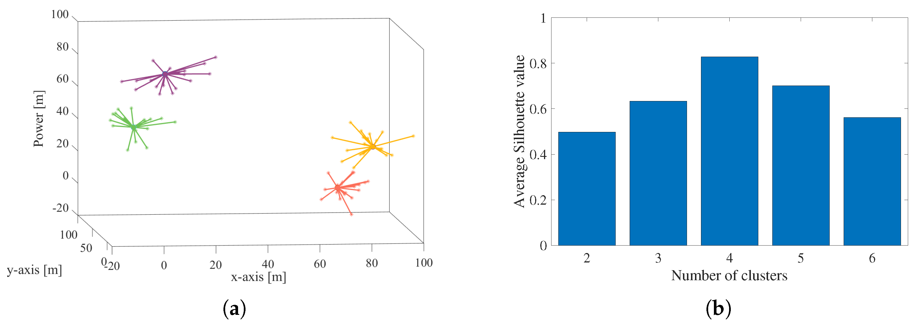
• A FANET clustering algorithm is proposed in this paper. First, the Silhouette coefficient is used to determine the number of clusters for given nodes’ positions and velocities. It aims to find an optimal number of clusters with the highest average coefficient value. Then, the k-means++ algorithm is used to group all nodes into clusters periodically. When calculating nodes’ distance, both position and velocity differences are considered. Moreover, the CHs of the previous iteration are used to initialize the centroids of the current iteration.
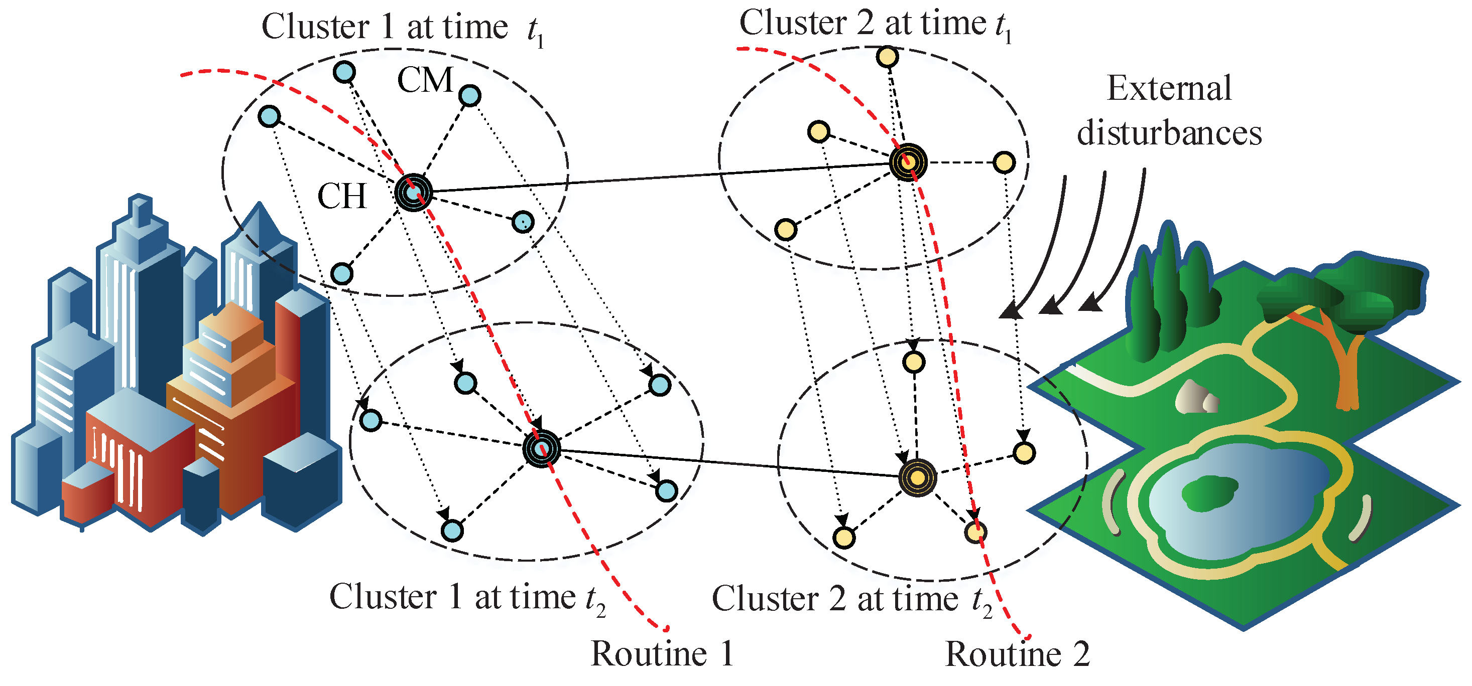
• A high-mobility FANET networking scheme is proposed based on the linear Kalman filter. To model nodes’ mobility influenced by external interferences, we use the Gaussian–Markov process to characterize nodes’ mobility influenced by external interferences. Specifically, we establish the state transfer relationship of position and velocity between two adjacent times and the Kalman. On this basis, the Kalman filter is utilized to predict the positions and velocities of all nodes.
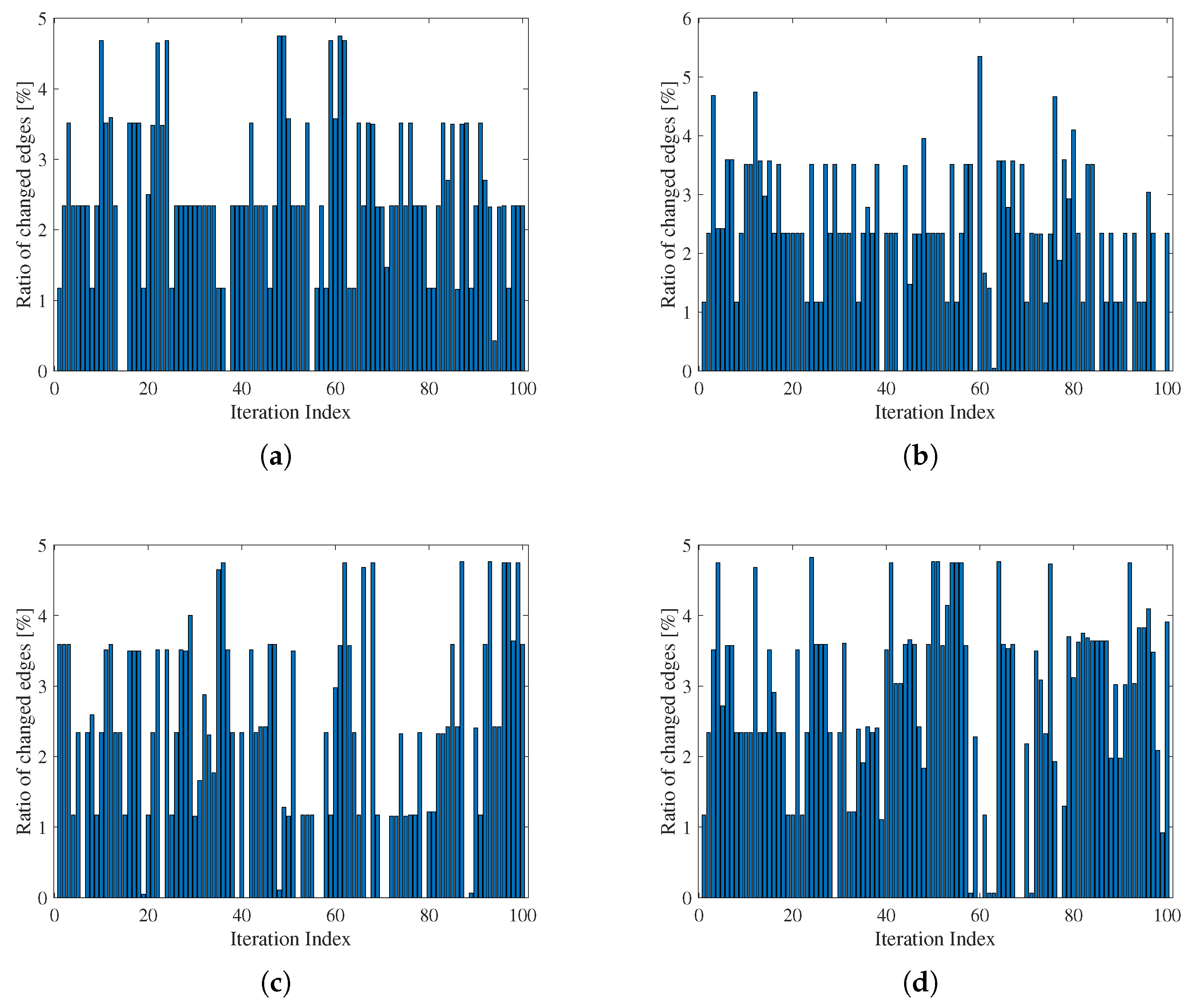
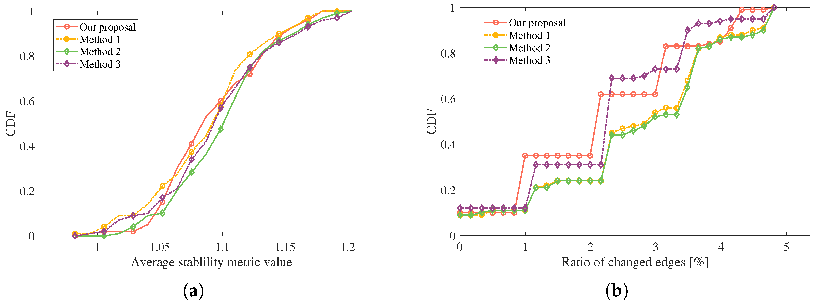
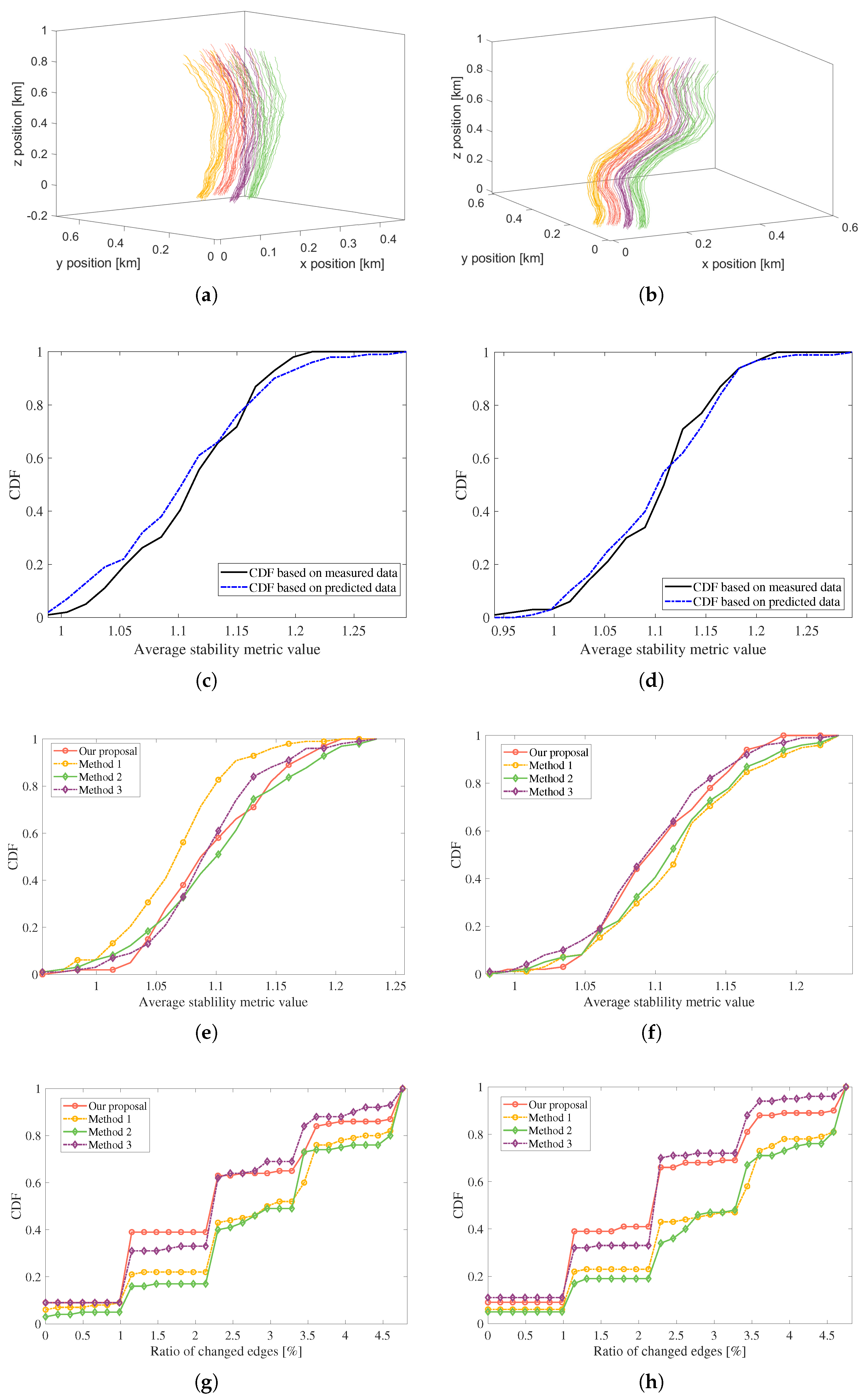
• This paper further evaluates the networking performance from three aspects, i.e., the cluster stability, ratio of changed edges based on the abstracted graph and computational complexity. The first metric measures the relative position and velocity difference within a cluster, whereas the second metric reflects the required communication overhead costs during the network evolution.
• Extensive simulations are conducted to evaluate the performance of our proposal under different node trajectories and velocities. Thereafter, we compare it with the existing FANET networking algorithms. The simulation results show that the proposed scheme outperforms the conventional schemes marginally from the aspects of cluster stability coefficient and ratio of changed edge numbers. Nonetheless, it presents a relatively low computational complexity in contrast to other algorithms; this implies that the proposed scheme is applicable in high-mobile scenarios, which require fast and reliable networking.

The remainder of this paper is outlined as follows. Section 2 present a review of related work. In Section 3, we describe the stochastic mobility model of the FANET node and introduce the prediction method based on the Kalman filter. In Section 4, the clustering method based on k-means++ is elaborated, and the performance evaluation metric includes cluster stability and overhead cost. The simulation and numerical results are presented and discussed in Section 5. Relevant conclusions are finally drawn in Section 6.

2. Review of Related Works

The ad hoc network mobility models serve as the cornerstones of network design, performance evaluation and routing protocols design, etc. For example, Wan et al. in [5] proposed a smooth turn mobility model, which can capture the acceleration correlation for UAVs over different time and positions while failing to consider the randomness. Currently, extensive studies have been conducted and some random mobility models have been proposed, such as the widely used random walk (RW), random direction (RD), random waypoint (RWP) models [6,7]. Specifically, the RWP model assumes that all nodes are independent and nodes are assigned with random destinations and velocities. Once arriving, they pause for a random break before proceeding to the next random destination. These works take the stochastic process into account to emulate the random deviation or jitter due to external interference. Nevertheless, they fail to depict the correlation between two adjacent times. In other words, the speed is influenced by the previous state. In [8], Camp et al. summarized the mobility models that are widely used in the simulations of ad hoc networks, including the Gaussian–Markov model, which model current speeds and movement directions based on the corresponding former speeds and directions.

The network topology architecture is a foundation for further FANET management, and unreasonable networking may increase the communication overheads, and even jeopardize or paralyze the entire network. Considering the existence of multiple mobile nodes, considerable researchers have focused on it and proposed some classical models. In [1], Xiao et al. summarized the three typical network topologies of FANET, i.e., the star topology, mesh topology, and the cluster-based hierarchical topology. In contrast to the star topology structure, the mesh topology possesses merits of high flexibility and autonomy and it can overcome the high link path loss or interruptions in some harsh scenarios via multiple hops. However, it requires quantities of overheads to realize data packet transmission via multiple hops. Regarding the cluster-based networking methods, this hybrid hierarchical topology can evidently reduce the management complexity and communication overheads. Furthermore, this scheme can group nodes into different clusters based on different application scenarios and arrangement strategies. Nonetheless, it encounters some new challenges, such as the determination of number of cluster and the election of CH. In [9], Shao et al. proposed a border patrol clustering algorithm (BPCA) via a cooperative architecture, which optimizes the CH selection by taking the effects of relative speed, separation distance, and nodes’ movement model into account. In [10], Tropea et al. introduced a FANET simulator, which considers human mobility behaviors, UAV/drone behavior models, and energetic issues.

In highly mobile scenarios, the network needs frequent updates to maintain a stable structure, which leads to an increase in control overhead and transmission latency. To tackle the mobile scenario, the authors in [11] proposed a FANET clustering algorithm based on the k-means model. It considers both the mobility and relative positions to boost the network reliability. Furthermore, the authors derived the optimal cluster sized based on the maximum coverage probability of CH. In [12], Wang et al. determined the cluster number based on bandwidth balance and used the k-means algorithm to group all nodes. Then, they proposed a deep Q-learning (DQN)-based cluster head selection algorithm. Another promising method is to predict the node information to assist further clustering. For example, Zang et al. in [13] proposed a mobility-prediction-based clustering algorithm by using the attributes of moving UAVs. Specifically, they presented a dictionary trie structure prediction algorithm and link expiration time mobility model. In [14], Cai et al. proposed a clustering algorithm by considering the residual energy, relative velocities difference and connections with neighbor nodes. Furthermore, a novel group mobility metric combining the instantaneous velocities and directions is proposed. To better highlight our contribution, a table-based comparison is presented in

Table 1. Comparison among different references.

Citation	Networking Method	Clustering Metric
[9]	border patrol clustering algorithm	relative speed and separation distance
[11]	k-means	mobility and relative positions
[12]	k-means	bandwidth balance
[13]	weighted clustering algorithm	node mobility, connectivity degree, total distance to neighbors, and consumed battery power
[14]	group mobility based clustering algorithm	residual energy, relative velocities difference, and connections with neighbor nodes
[15]	hybrid gray wolf optimization method	inter-cluster distance, intra-cluster distance, residual energy, and geographic location
[16]	bio-inspired localization and clustering schemes	cluster building time, number of clusters, cluster lifetime, and energy consumption

.

3. Location and Velocity Prediction

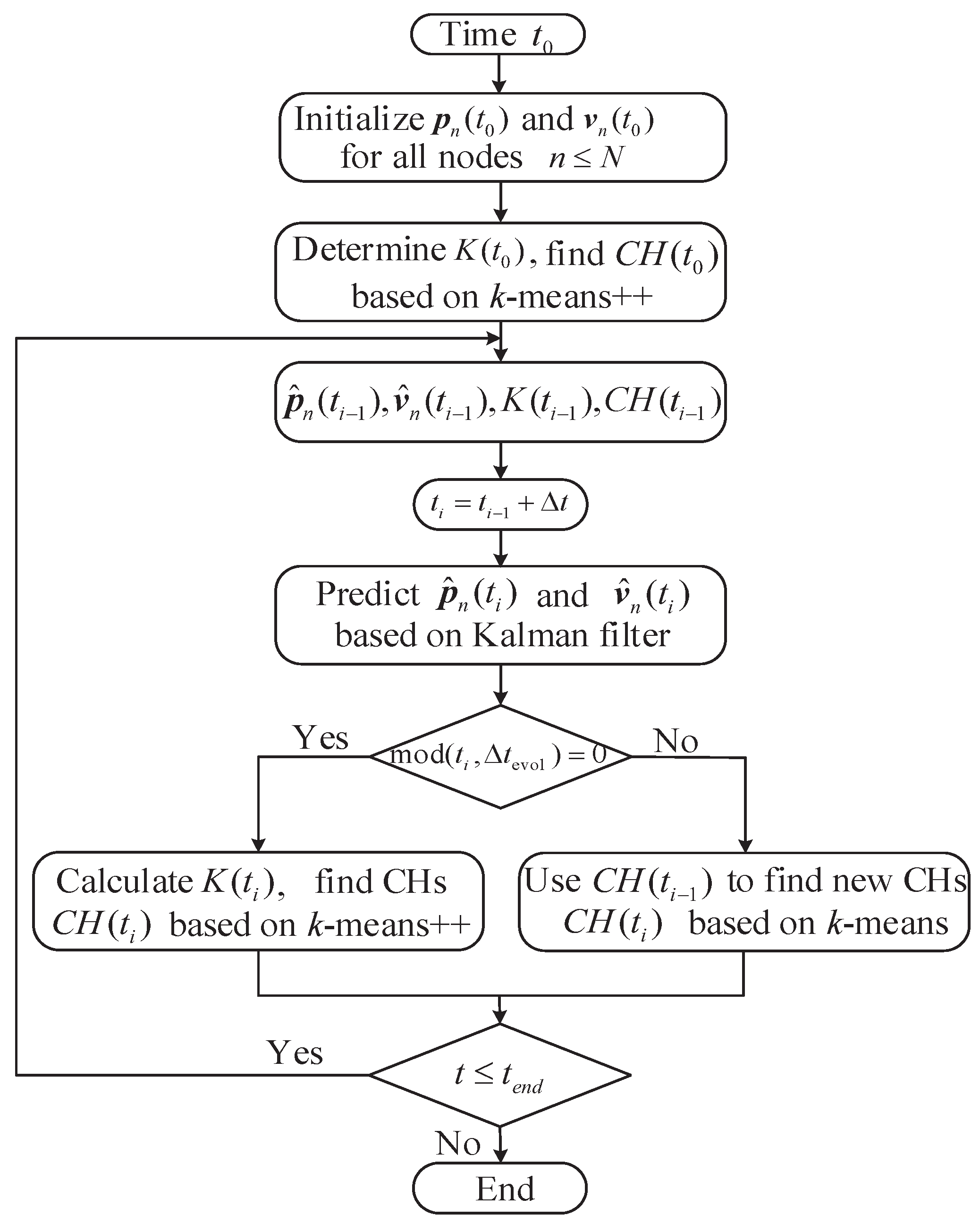
3.1. Framework of the Proposed Algorithm

In this section, we will introduce the Kalman-filter-assisted prediction of nodes’ information for the FANET. To start with, the procedure flowchart of our proposed algorithm is presented in Figure 2 and we will elaborate each step in detail in the following text. Our proposed algorithm mainly contains the following three steps, which are

• Initialize the simulation parameter settings at time $t_0$, including the total node number, nodes’ locations and velocities. Determine the number of cluster $K\left(t_0\right)$ by using the Silhouette coefficient and group all nodes into clusters. Find the CH for each cluster based on the k-means++ algorithm.
• Predict the node location ${\widehat{\mathit{p}}}_n\left(t_i\right)$ and velocity ${\widehat{\mathit{v}}}_n\left(t_i\right)$ based on the Kalman filter. Cluster all nodes based on the predicted information via k-means or k-means++ algorithm. Update simulation time $t_i\leftarrow t_{i-1}+\Delta t$.
• Repeat step 2 until the preset simulation time $t_{end}$ is reached or other convergence conditions are satisfied.

3.2. Initialization and Modeling of Node Movement

First, we generate several stochastically distributed nodes with high mobility based on the Gaussian mixture distribution. Specifically, we set a number of cluster $K\left(t_0\right)$ at the initial simulation time $t_0$. For the i-th node belonging to the k-th cluster, marked as $n_{k,l}$ in brief, we assume that the corresponding location obeys the three-dimensional (3-D) Gaussian distribution, i.e., $\mathit{p}\left(n_{k,i}\right)\sim \mathcal{N}({\mu }_k,{\mathsf{\Sigma }}_k)$, where ${\mu }_k$ and ${\mathsf{\Sigma }}_k$ represent the average location matrix and the covariance matrix, respectively. Regarding the initial movement speed $\mathit{v}\left(t_0\right)$, it is assumed that all nodes proceed in a direction with the same speed $v_0$ at the initial simulation time $t_0$.

During the proceeding process, nodes are expected to travel along the pre-defined trajectories. However, they may be influenced by external obstacles, winds and other airflow interferences, etc., presenting stochastic mobility processes consequently. To depict this feature of all network nodes, we adopt the Gauss–Markov mobility model (GMMM), which can be adapted to various levels of randomness by tuning a single parameter [8]. However, when applying this model in a network with a bunch of nodes, it assumes every node is completely independent of another. Hence, it fails to model those nodes’ mobility behaviors that move together or in groups. Therefore, we combine the GMMM with a group mobility model, namely the reference point group mobility (RPGM) model [17]. Specifically, our proposal mainly contains two phases, i.e.,

• Generate group center nodes and model their movements based on GMMM. First, initialize the center nodes with given positions, velocities, and moving directions at the initialization time $t_0$. Then, update these three parameters based on the following three equations, which are

  $$v\left(t_k\right)=\alpha v\left(t_{k-1}\right)+(1-\alpha )\overline{v}+\sqrt{(1-{\alpha }^2)}{v}_{x_{k-1}},$$

  (1)

  $$\theta \left(t_k\right)=\alpha \theta \left(t_{k-1}\right)+(1-\alpha )\overline{\theta }+\sqrt{(1-{\alpha }^2)}{\theta }_{x_{k-1}},$$

  (2)

  $$\varphi \left(t_k\right)=\alpha \varphi \left(t_{k-1}\right)+(1-\alpha )\overline{\varphi }+\sqrt{(1-{\alpha }^2)}{\varphi }_{x_{k-1}},$$

  (3)

  where $v\left(t_k\right)$ means the moving speed at time $t_k$, $\overline{v}$ is a constant, which denotes the average speed and $v_{x_{k-1}}$ is a random variable following the Gaussian distribution. $\alpha$ is a parameter that controls the movement randomness. Specifically, the case of $\alpha =0$ represents a totally random process, i.e., the Brownian motion, whereas the case of $\alpha =1$ means a completely deterministic process.
  Since flying nodes are moving in 3-D Euclidean space, we use two angular variables to depict the movement direction. Variables $\theta$ and $\varphi$ denote the elevation and azimuth angles of the speed vector, respectively. The meanings of variables $\overline{\theta }$, $\overline{\varphi }$, ${\theta }_{x_{k-1}}$, and ${\varphi }_{x_{k-1}}$ are similar to those of Equation (1). Finally, the location at time $t_k$ can be obtained based on the previous location, speed and moving direction at time $t_{k-1}$, which are

  $$\left(\begin{array}{c}{p}_x\left(t_k\right)\\ p_y\left(t_k\right)\\ p_z\left(t_k\right)\end{array}\right)=\left(\begin{array}{c}{p}_x\left(t_{k-1}\right)\\ p_y\left(t_{k-1}\right)\\ p_z\left(t_{k-1}\right)\end{array}\right)+\left(\begin{array}{c}cos\varphi \left(t_{k-1}\right)sin\theta \left(t_{k-1}\right)\\ sin\varphi \left(t_{k-1}\right)sin\theta \left(t_{k-1}\right)\\ cos\theta \left(t_{k-1}\right)\end{array}\right)v\left(t_{k-1}\right)\Delta t,$$

  (4)

  where $\Delta t$ is the updation time interval. Note that $p_x$, $p_y$, and $p_z$ are the corresponding x, y and z coordinates of the node’s position, respectively.
• As for each group center, generate some nodes around the center randomly, of which locations are assumed to obey the Gaussian distribution, and their centers are set as the mean values. Their locations and velocities are derived based on the corresponding centers. According to [8], the velocity ${\mathit{v}}_{k,i}$ of node $n_{k,i}$ belonging to the k-th group can be obtained by adding a random motion vector $\Delta {\mathit{v}}_{r,i}$ to the center speed vector ${\mathit{v}}_k^C$ as shown in Figure 3.
  This relationship between group center and member velocities can be expressed as

  $${\mathit{v}}_{k,i}={\mathit{v}}_k^C+\Delta {\mathit{v}}_{r,i},$$

  (5)

  $$\Delta {\mathit{v}}_{r,i}=v_r\left(\begin{array}{c}cos{\varphi }_{r}sin{\theta }_r\\ sin{\varphi }_{r}sin{\theta }_r\\ cos{\theta }_r\end{array}\right),$$

  (6)

  where $v_r$ is distributed uniformly within a specified maximal speed $v_{r,\max }$, i.e., $v_r\in [0,v_{r,\max }]$. The random elevation ${\theta }_r$ angle is uniformly distributed within $(0,2\pi ]$ and the azimuth angle ${\varphi }_r$ varies evenly within a range of $(0,\pi ]$.

3.3. Kalman-Filter-Based Trajectory Prediction

The trajectories of network nodes are pivotal to further system optimization and routing protocol design. However, the movement of nodes is easily influenced by external disturbances such as noise, airflow interference, etc., which causes deviations from the intended paths. Specifically, all nodes need to broadcast messages periodically to exchange position information with surrounding nodes. In highly mobile scenarios, this procedure is frequently conducted, creating quantities of overheads consequently. To handle this issue, we adopt the Kalman filter to predict the node trajectories, aiming to reduce the overheads with aid of predicted location and velocity. Kalman filter is a recursive solution to the discrete data linear filtering problem [18]. With high prediction accuracy and low computational complexity, it has been used in extensive research and applications, such as control, navigation, filtering, etc. Some works have implemented it in the ad hoc network, e.g., the authors in [19] used the Kalman filter to estimate the cooperative awareness messages (CAMs). The main procedure of the Kalman filter contains two phases, i.e., time updation and measurement updation. The time updation contains two formulas, which are

$${\widehat{\mathit{x}}}_k^{-}=\mathit{A}{\widehat{\mathit{x}}}_{k-1}+\mathit{B}{\mathit{u}}_{k-1},$$

(7)

$${\mathit{P}}_k^{-}=\mathit{A}{\mathit{P}}_{k-1}{\mathit{A}}^T+\mathit{Q},$$

(8)

where the superscript “−” indicates that vectors are obtained before the measurement, symbol hat notation “$\widehat{·}$” indicates the estimated results. Hence, ${\widehat{\mathit{x}}}_k^{-}$ is the estimated state at the k-th step based on the prior process to the current step. ${\widehat{\mathit{x}}}_k$ means the estimated posterior state at the k-th step based on the current measured result ${\mathit{z}}_k$. State transfer matrix $\mathit{A}$ relates two adjacent states of previous and current steps, and input matrix $\mathit{B}$ relates the control input ${\mathit{u}}_{k-1}$ to state $\mathit{x}$. ${\mathit{P}}_k^{-}$ and ${\mathit{P}}_k$ denote the prior and posterior estimated error covariances, respectively. $\mathit{Q}$ is the process noise covariance matrix.

As for the measurement updation, it includes the following three equations, i.e.,

$${\mathit{K}}_k={\mathit{P}}_k^{-}{\mathit{H}}^T{\left(\mathit{H}{\mathit{P}}_k^{-}{\mathit{H}}^T+\mathit{R}\right)}^{-1},$$

(9)

$${\widehat{\mathit{x}}}_k={\widehat{\mathit{x}}}_k^{-}+{\mathit{K}}_k\left({\mathit{z}}_k-\mathit{H}{\widehat{\mathit{x}}}_k^{-}\right),$$

(10)

$${\mathit{P}}_k=\left(\mathit{I}-{\mathit{K}}_k\mathit{H}\right){\mathit{P}}_k^{-},$$

(11)

where ${\mathit{K}}_k$ means the Kalman gain at the k-th step, measurement matrix $\mathit{H}$ relates the state ${\mathit{x}}_k$ to the measured value ${\mathit{z}}_k$ and $\mathit{R}$ is the measurement noise covariance matrix. The time-updating procedure aims to predict states, whereas the measurement updating procedure tries to correct the state based on current measurement results. By using these two recursive procedures, the Kalman filter can realize high-precision prediction with low computational cost.

In this paper, the Kalman filter is utilized to predict the velocities and positions of all nodes in highly mobile scenarios. Consequently, we take these two key variables into account and combine them into a state $\mathit{x}$ with an expression of $\mathit{x}={[p_x,p_y,p_z,v_x,v_y,v_z]}^{\mathsf{T}}$. As for the input matrix $\mathit{B}$, it is set to $\mathbf{0}$ since no external input is considered for this case. Based on the relationship between position and velocity, the state transfer matrix $\mathit{A}$ can be presented as

$$\mathit{A}={\left(\begin{array}{cc}{\mathit{I}}_{3\times 3}& \Delta t{\mathit{I}}_{3\times 3}\\ {\mathbf{0}}_{3\times 3}& {\mathit{I}}_{3\times 3}\end{array}\right)}_{6\times 6}.$$

(12)

On this basis, we can predict the positions and velocities for all nodes via the previous prediction and current measurement results.

4. Network Clustering

4.1. Number Determination of Clusters

Based on the estimated information of positions and velocities, we aim to group these nodes into several clusters by using the k-means++ algorithm, which is an unsupervised learning method [20]. Before performing clustering, it is essential to determine the cluster number. Herein, we adopt the widely used Silhouette coefficient, which does not need to know the labeling of the dataset [21,22]. It gives a metric of the separation between clusters and thus provides a way to assess the number of clusters. For each node, the corresponding Silhouette coefficient is expressed as

$$s\left(i\right)=\frac{b\left(i\right)-a\left(i\right)}{max\left\{a\right(i),b(i\left)\right\}},$$

(13)

where $a\left(i\right)$ is the average distance between node $n_i$ and the rest members belonging to the same cluster, $b\left(i\right)$ denotes the average distance between node $n_i$ and all other members belonging to the nearest cluster. The detailed expressions of $a\left(i\right)$ and $b\left(i\right)$ are presented as

$$a\left(i\right)=\frac{1}{\left|C\right(i\left)\right|-1}\sum _{C\left(i\right),i\ne j}D(i,j),$$

(14)

$$b\left(i\right)=\underset{i\ne j}{min}\{\frac{1}{\left|C\right(j\left)\right|}\sum _{j\in C\left(j\right)}D(i,j)\},$$

(15)

where $\left|C\right(i\left)\right|$ is the total member number belonging to the cluster assigned to $n_i$. According to Equation (13), it can be learned that this metric has a range of [−1, 1]. To determine the optimal number of clusters, we iterate different numbers of cluster and calculate the average silhouette coefficient of all nodes for a given number of cluster. The number with the maximum value is regarded as the optimal choice. Furthermore, multiple rounds are conducted and the average number is used to eliminate the randomness error.

4.2. k-means+ Clustering Algorithm

Since the k-means algorithm is sensitive to the initialization of the centroids, we utilize the k-means++ to overcome this drawback. The k-means++ algorithm mainly contains the following three steps [23].

• Choose a node from the set $\mathcal{X}$ randomly as the centroid of the 1st cluster, marked as $c_1$.
• For a node marked as $n_i(i\in \mathcal{X})$, calculate its distance from the nearest previously chosen centroids and obtain the distance vector. It can be expressed as

  $$D\left(i\right)=\underset{k\in \mathcal{K}}{min}\left\{D(i,k)\right\},$$

  (16)

  where $\mathcal{K}$ is a set containing all previously chosen centroids.
• Choose a node $n_j\in \mathcal{X}$ as the centroid of next cluster with a probability of

  $$P\left(j\right)=\frac{D^2\left(j\right)}{{\sum }_{n_j\in \mathcal{X}}{D}^2\left(j\right)},$$

  (17)
  This formula implies that the probability of a node being selected as the next centroid is highly related to its separation from the nearest, previously chosen centroid.
• Repeat Step 2 and Step 3 until K centroids have been determined.
• Use the k-means algorithm to cluster all nodes and obtain the centroids.
• For the k-th cluster, search a CM from the assigned CMs ${\mathcal{X}}_k$ with the nearest distance to the centroid $c_k$ and take it as the CH, i.e.,

  $$C{H}_k=arg\underset{k\in {\mathcal{X}}_k}{min}\{\parallel \mathit{p}\left(k\right)-{\mathit{c}}_k\parallel \}.$$

  (18)

It is noteworthy that the distance between any two nodes, namely $n_i$ and $n_j$, during the clustering procedure not only depends on their relative positions but also is related to their relative speed differences, which can be expressed as

$$D(i,j)=\parallel {\mathit{p}}_i-{\mathit{p}}_j\parallel +\Delta t\parallel {\mathit{v}}_i-{\mathit{v}}_j\parallel ,$$

(19)

where symbol $\parallel ·\parallel$ calculates the 2-norm, i.e., the 3-D Euclidean distance. The second part of this equation indicates a possible separation distance at a short update interval $\Delta t$. Hence, this equation implies that a higher speed difference should not be ignored even under the case of close position distance.

As for the convergence condition, it contains the judgment of maximal iteration and CH position difference, which proceeds as follows: (1) If current iteration reaches the pre-set maximal iterations, then it will stop regardless of the position difference. This condition is set to cater to the requirement of low computational time for highly mobile scenarios. (2) If the cluster head position differences between the pre-iteration and current iteration are smaller than the given threshold, then it will stop.

4.3. Dynamic Clustering Evaluation

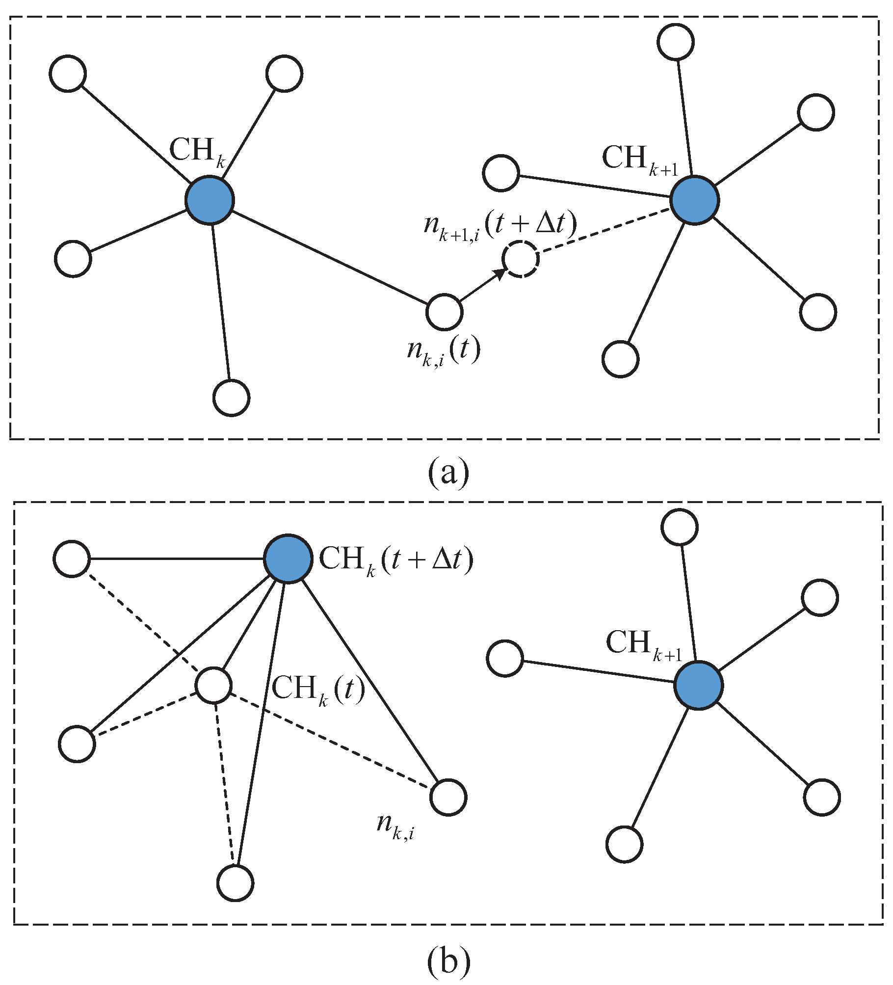
4.3.1. Communication Overhead Metric

In our proposal, the network is established based on the concept of cluster intending to manage nodes separately and autonomously [24]. The clustering algorithm is usually conducted based on some metrics such as Euclidean distance, cosine distance, Hamming distance, etc. For a given cluster, it consists of a CH and several nearby cluster members (CMs) which are reachable from the CH by single or multiple hops. As such, they need to exchange messages periodically to maintain the existing topology or form a new one. The number of changed edges is highly related to the communication overheads. If a link connecting two nodes breaks, the involved nodes will send cooperative awareness messages (CAMs), containing key safety-related information such as speed and position, and they wait responses from the nearby nodes. Then, a new link will be established with another CH. It can be seen that the new link is established at a cost of additional CAMs. The more links change, the more CAMs are required. Consequently, it is reasonable to use the number of changed links to measure the communication overheads in this paper. Nonetheless, mobile nodes cause time-varying network topology, especially in high-mobility scenarios, yielding rapid cluster stability degradation. As such, it is essential to check and update the network topology periodically and select new CHs for a purpose of adapting to new environments.

Generally speaking, the topology variation contains the CM change case and the CH change case. As shown in Figure 4a, for a given topology structure at time t, assume two clusters are constructed and the node $n_{k,i}\left(t\right)$ is grouped into the k-th cluster at time t. As time proceeds, node $n_{k,i}\left(t\right)$ moves forward to a new position, which will be classified into the $(k+1)$-th cluster, denoted as $n_{k+1,i}(t+\Delta t)$. To complete this procedure, the CHs of these involved two clusters need to exchange control overheads. The second case involving the change of CH is presented in Figure 4b, which indicates the CH of the k-th cluster changes from time t to $t+\Delta t$. Obviously, this case results in more changed links. For instance, a new single-hop link needs to be established in Figure 4a, whereas four new single-hop links are involved in Figure 4b. Assuming the communication overhead cost is proportional to the number of changed links, we consequently focus on this aspect during the mobile process in the following text.

To quantify the changed link number, we abstract the topology into an undirected graph with an expression of $\mathcal{G}=\{V,E\}$ herein, where V means the vertex set of all nodes, and E is the edge set connecting two adjacent nodes. To depict the connection relationship between nodes, we establish a binary connection matrix with an expression of $C={\left[c_{ij}\right]}_{N\times N}$. As for the matrix element $c_{ij}$, its value is set according to nodes’ connection relationships, i.e.,

$$c_{ij}=\left\{\begin{array}{c}\hfill 0n_i\nleftrightarrow n_j\\ \hfill 1n_i\leftrightarrow n_j\end{array}\right.$$

(20)

Obviously, if node $n_i$ is connected to $n_j$ directly, then $c_{ij}=1$. Otherwise, $c_{ij}=0$. On this basis, the changed edge can be found by comparing two adjacent connection matrices, which is

$$\mathit{D}(t,t+\Delta t)=\mathit{C}\left(t\right)\oplus \mathit{C}(t+\Delta t),$$

(21)

where symbol “⊕” is the exclusive or operator. Since the connection matrix $\mathit{C}$ is symmetric, the changed edge number from time t to $t+\Delta t$ can be expressed as

$$N_c=card\{\mathit{D}\ne 0\}/2,$$

(22)

where function $card\{·\}$ calculates the cardinal number of a set. The worst case happens when the updated graph is totally different from the previous one, hence we use the ratio of changed edge number to depict the evolution situation, which is about

$$\gamma =\frac{N_c}{C_N^2},$$

(23)

where N represent the total node number, $C_N^2$ is the number of combinations.

4.3.2. Cluster Maintenance Metric

To characterize the cluster maintenance, Rossi et al. in [25] took both the relative mean speed $S_k$ and distance $D_k$ into account and proposed a novel CH selection index to evaluate the cluster maintenance in three-dimensional (2-D) Euclidean space. In this paper, we extend it to the 3-D Euclidean space. For a node $n_{k,i}$ belong to the k-th cluster ${\Phi }_k$, its cluster maintenance metric ${\xi }_{k,i}$ can be expressed as

$${\xi }_{k,i}=S_{k,i}+D_{k,i},$$

(24)

$$S_{k,i}=\frac{{\sum }_{j=1}^{N_k}\parallel {\mathit{v}}_{k,i}-{\mathit{v}}_{k,j}\parallel }{N_{k}max\left\{{\Omega }_{k,i}\right\}}$$

(25)

$$D_{k,i}=\frac{{\sum }_{j=1}^{N_k}\parallel {\mathit{p}}_{k,i}-{\mathit{p}}_{k,j}\parallel }{N_{k}max\left\{Z_k\right\}}$$

(26)

where ${\Omega }_{k,i}$ denotes the speed difference set among different nodes within the cluster set ${\Phi }_k$ and it is calculated by

$${\Omega }_{k,i}=\{\parallel {\mathit{v}}_{k,i}-{\mathit{v}}_{k,j}\parallel |\forall n_{k,j}\in {\Phi }_k.$$

(27)

$N_k$ is the element number of ${\Phi }_k$. Set $Z_{k,i}$ consists of all Euclidean distances between CMs of ${\Phi }_k$ and node $n_{k,i}$ and it can be calculated as

$$Z_{k,i}=\{\parallel {\mathit{p}}_{k,i}-{\mathit{p}}_{k,j}\parallel |\forall n_{k,j}\in {\Phi }_k\}.$$

(28)

Based on Equation (24), we can learn that the value of ${\xi }_k$ varies within the range of $[0,2]$. Calculate the stability metric values for those nodes belonging to ${\Phi }_k$, and take the average value as the cluster maintenance metric, which is expressed as

$${\xi }_k=\sum _i{\xi }_{k,i}/N_k.$$

(29)

5. Simulation and Analysis

In this section, we will present a series of simulation works to verify our proposed network clustering algorithm. The simulation scenario is set to a mobile UAV FANET scenario, where a swarm of UAVs proceeds at high mobility. Note that all nodes are at high altitudes and there are no obstacles around them. They proceed at predefined trajectories with influences from external winds and currents, which causes deviations from routines. Hence, their corresponding node motions are characterized by the proposed RPGM. Furthermore, higher motion velocity causes more severe disturbances to both positions and speeds. Nodes send CAMs periodically to maintain the topology structure. Once a link is disconnected, then a bunch of CAMs are required to establish a new link. The simulation is performed on the MATLAB platform in a Windows operating system. To start with, we set the initialization number of clusters $K\left(t_0\right)$ as 4 and generate 20 nodes per cluster randomly. Then, we initialize the node locations based on the Gaussian distribution with mean positions of $(0,0,80)$ m, $(0,80,40)$ m, $(80,0,40)$ m, and $(80,80,0)$ m, respectively. All nodes move in the same direction of $({\varphi }_0,{\theta }_0)=({45}^{\circ },{45}^{\circ })$ at the initial time $t_0$. The RPGM is used to model the movement of all nodes and the initialized group center speed is 30 m/s. The maximal random speed is set to 3 m/s. On this basis, the proposed Kalman-filter-assisted networking algorithm is utilized to reduce communication overheads. The detailed simulation parameter values are presented in

Table 2. Simulation settings.

Parameters	Values	Parameters	Values
$\alpha$	0.5	$\overline{\theta }$	${10}^{\circ }$
$\overline{v}$	5 m/s	$\overline{\varphi }$	${10}^{\circ }$
Initial direction $({\varphi }_0,{\theta }_0)$	$({45}^{\circ },{45}^{\circ })$	Updation interval $\Delta t$	0.1 s
Evolution interval $\Delta t_{\mathrm{evol}}$	0.4 s	Total simulation time	10 s
Initial number of clusters $K\left(t_0\right)$	4	Maximal random speed $v_{r,\max }$	3 m/s
Cluster center speed $v^C$	30 m/s	Number of node N	80
Initial ${\mathit{p}}_1^C$	[0, 0, 80] m	Initial ${\mathit{p}}_2^C$	[0, 80, 40] m
Initial ${\mathit{p}}_3^C$	[80, 0, 40] m	Initial ${\mathit{p}}_4^C$	[80, 80, 0] m

.

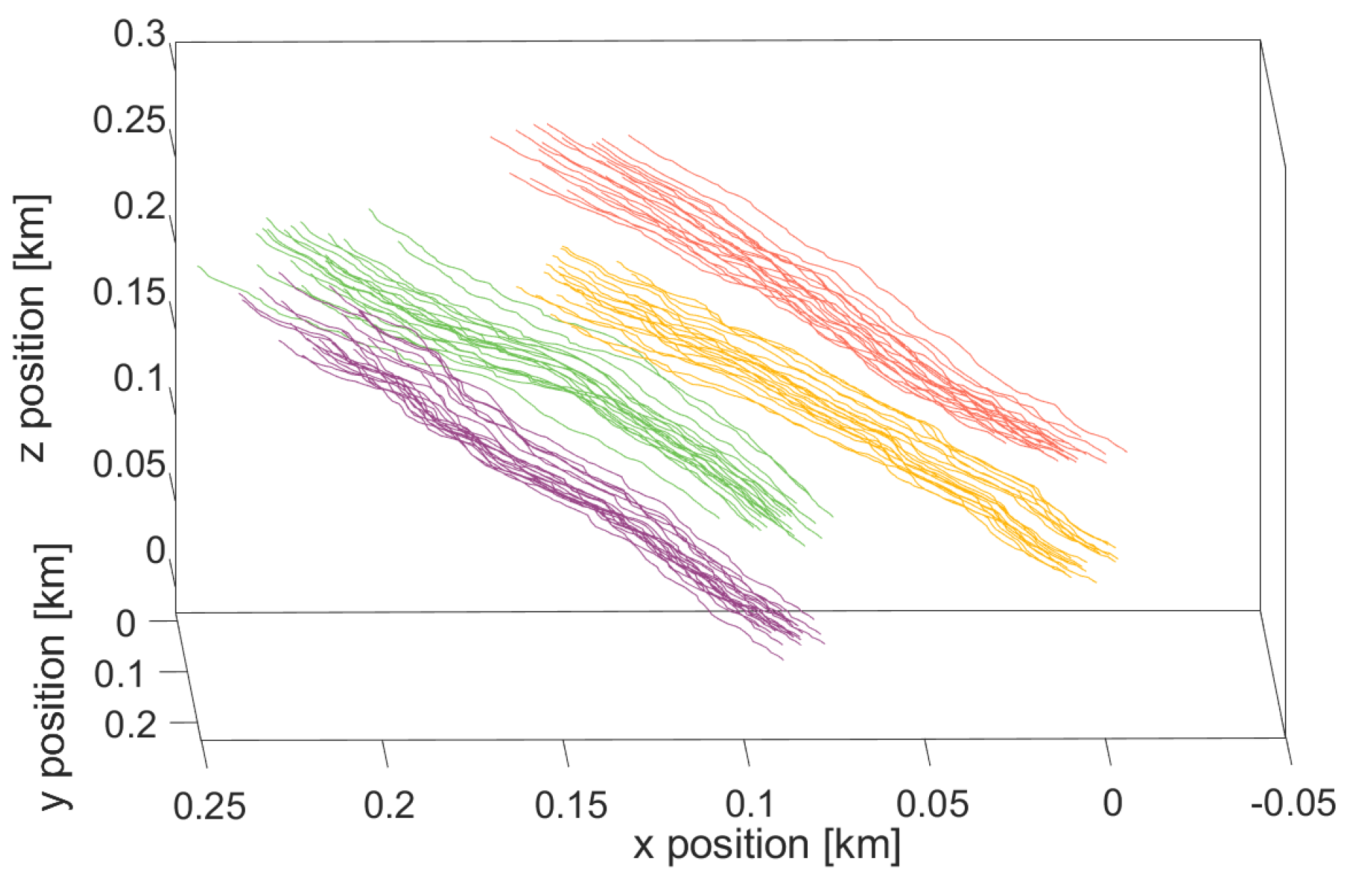
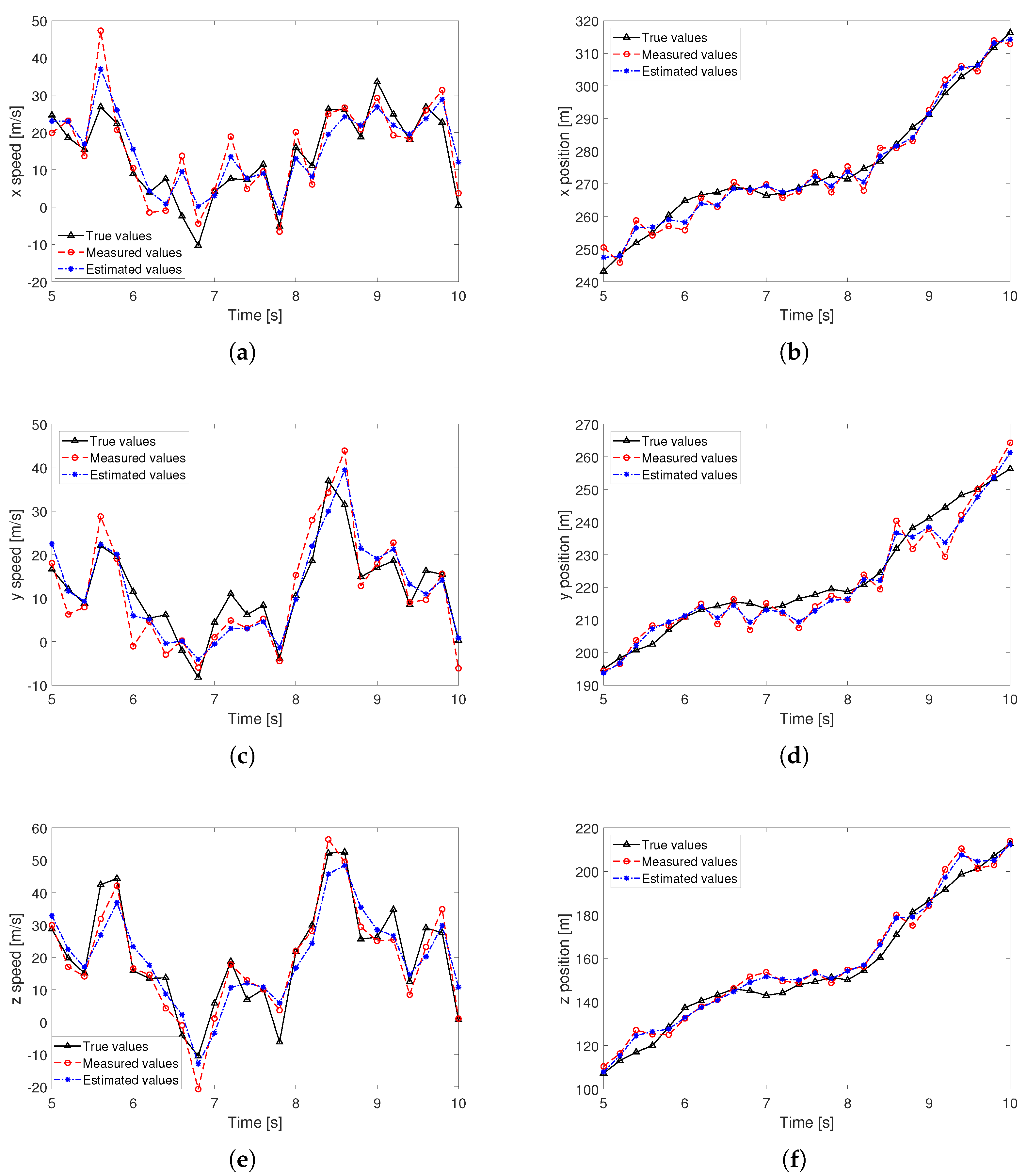
5.1. Node Initialization and Prediction

Figure 5a presents the initialized node positions. To determine the optimal number of clusters, we calculate the Silhouette coefficients over different numbers of clusters as shown in Figure 5b. It can be observed that the highest average value appears at the number 4, which corresponds to the preset number of clusters. Then, all nodes are grouped into discernible clusters based on the k-means++ algorithm. To better illustrate the clustering effects, nodes belonging to the same cluster are painted by the same color and lines connecting CMs and CH are also drawn. Obviously, four clusters can be identified and CHs lie at the center of clusters. Consequently, the nodes in Figure 5a are plotted in 4 different colors, where one color indicates one cluster.

Figure 6 plots the trajectories of all nodes during the whole simulation process, where curves of the same color represent trajectories belonging to the same cluster. It can be observed that nodes deviate slightly away from the desired paths as a result of external disturbances. Nonetheless, nodes belonging to the same cluster still gather together instead of moving in chaos and they can be separated with others easily. Hence, it implies that the proposed RGPM presents a good modeling capability of the group mobility.

Figure 7 presents the emulated trajectory of the 1st node from $t=5$ s to $t=10$ s, where Figure 7a,c,e denote the speed components on x, y and z axes. Figure 7b,d,f represent those of the position components. In these figures, the true data are denoted by black triangles, the measured data are obtained based on GPS and speed/acceleration sensors. They are marked by red circles. We can find some differences between true data and measured data, which stems from the white Gaussian noise. Furthermore, we plot the Kalman-filter-assisted prediction results, marked by blue stars. It can be learned that the prediction result presents a good fit to the measured results, even though the time-varying data are non-stationary. Then, the predicted data are utilized to assist the networking.

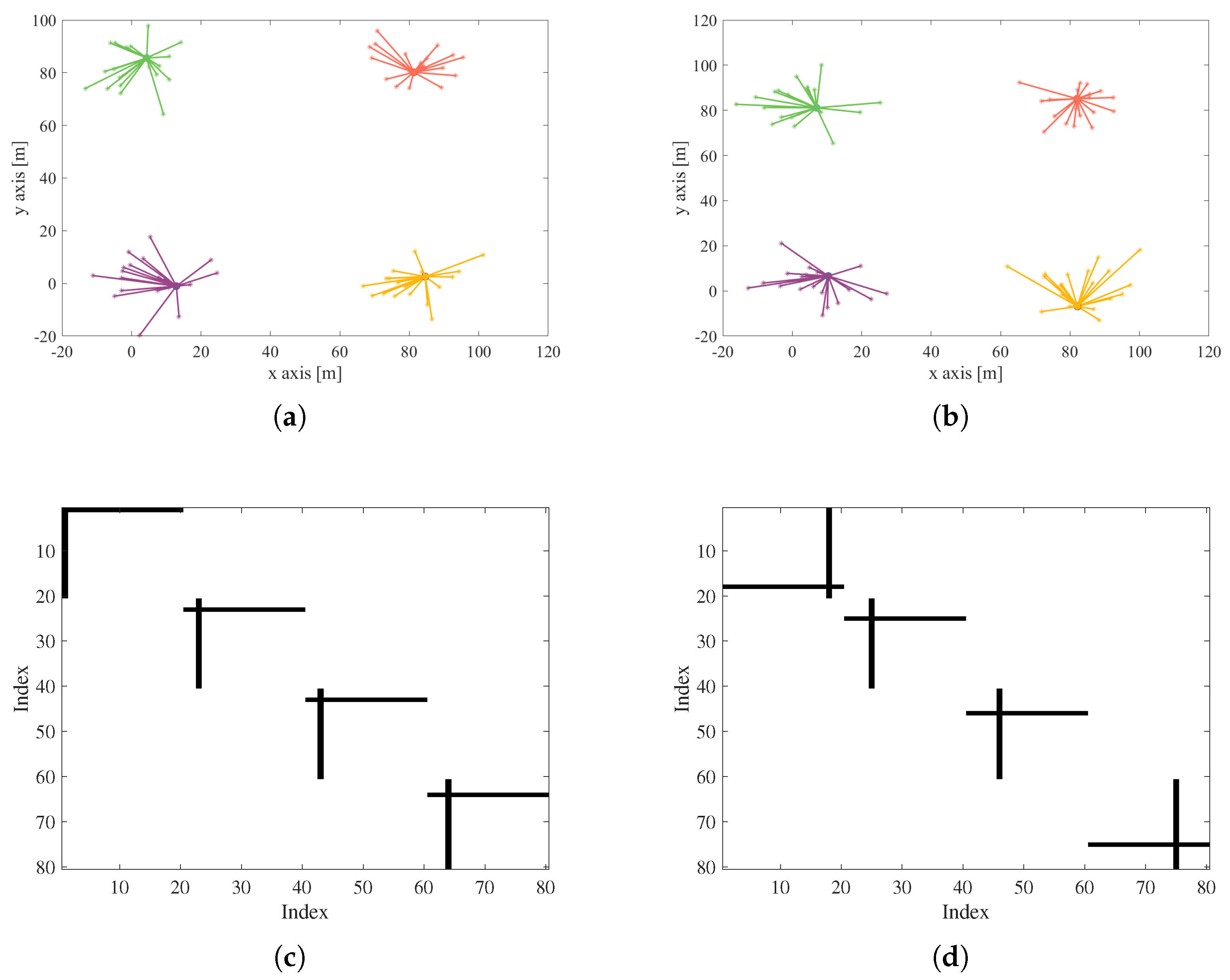
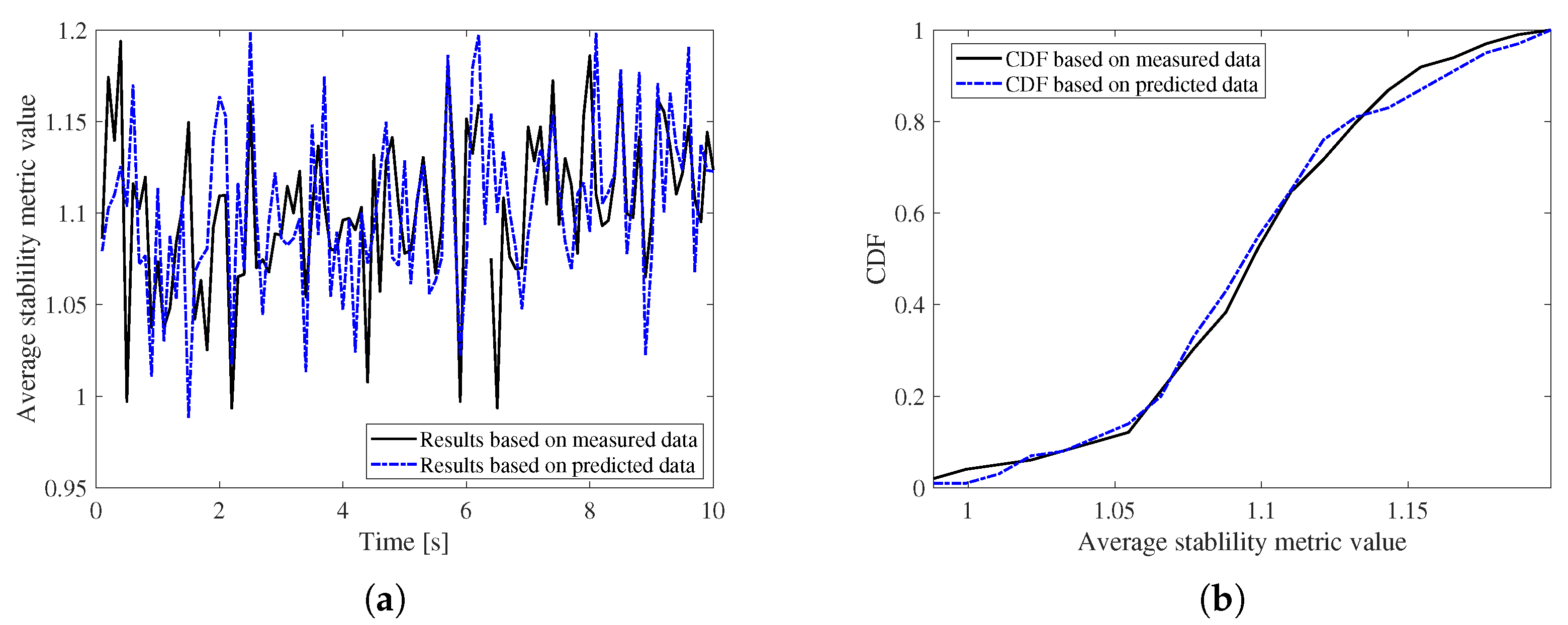
5.2. Performance Evaluation

Figure 8 presents a demonstration of the time-varying network topology, where Figure 8a,b denote two constructed topologies at two different times with an interval of $\Delta t=0.1$ s. The scatters plotted in one color belong to the same cluster and they are connected to a CH via edges with the same color. Figure 8c,d plot the corresponding graph matrices based on Equation (20). On this basis, the changed edge number can be easily calculated based on Equation (21). In Figure 8, we can find that the majority of the changed edges stem from the newly selected CH as a result of node movement, and no cross-cluster changed edges appear during this process.

Figure 9 plots the average stability metric results during the whole simulation, whereas Figure 9a plots the average stability metric values of all clusters at different time. In this figure, the black solid curve denotes the results based on the measured positions and velocities, whereas the dashed blue curve refers to that of the Kalman-filter-assisted estimated results. Obviously, the whole values of these two cases fluctuate around a value of 1. Figure 9b draws the corresponding cumulative distribution function (CDF) curves of these two data. It can be observed that the predicted results present a similar trend to the measured data, proving that our proposal can be used to assist the highly mobile FANET networking.

Figure 10 presents the ratio of changed edge number compared to the sensor measurement-based data over different group movement velocities, including 10 m/s, 30 m/s, 60 m/s, and 100 m/s. Moreover, we assume the maximal random speed $v_{r,\max }$ is proportional to the group speed $v^C$, implying that a higher $v^C$ is accompanied by more severe interferences. We can observe that the proposed algorithm can yield an overall ratio of 2–3% regardless of different group velocities, proving a good option to reduce communication overheads.

5.3. Comparisons with Existing Methods

We also compare with the existing algorithms to validate our proposal. Specifically, three different algorithms are compared, i.e., (1) Method 1: the conventional k-means algorithm is used. Note that the number of clusters is set to a constant of 4 during the whole simulation process. Moreover, the distance between nodes consists of their relative speed difference [25]. (2) Method 2: the method is similar to Method 1, but the distance between nodes does not consider the speed information [26]. (3) Method 3: the method is similar to Method 1, but it uses the k-means++ algorithm [27].

Figure 11a plots the stability CDF results of these 4 different algorithms during the whole simulation process at a speed of 30 m/s. It can be observed that these four algorithms show approximate performance, where Method 2 presents a slight advantage. Nonetheless, more comparisons using different metrics are needed to verify our proposal. Figure 11b plots the ratio CDF of the changed edges, where three different methods mentioned above are compared with our proposal. Generally, a smaller value of the ratio of changed edges implies a well-predicted network graph with respect to the actual network graph, resulting in fewer communication overheads consequently. From this figure, it can be seen that our proposal is slightly lower than these three algorithms, proving a good evolution performance.

The computational complexity of these four algorithms is compared in

Table 3. The computational complexity comparisons of different algorithms.

Algorithm	Computational Complexity	Time Consumption
Our proposal	$\mathcal{O}(\alpha kd{N}^2+(1-\alpha )kdN)$	0.93 s
Method 1	$\mathcal{O}\left(kdN\right)$	1.04 s
Method 2	$\mathcal{O}\left(kdN\right)$	0.51 s
Method 3	$\mathcal{O}\left(kd{N}^2\right)$	2.62 s

. The conventional k-means algorithm has a complexity of $\mathcal{O}\left(kdN\right)$ for each iteration, where N is the number of nodes, D is the number of dimensions, and k is the number of clusters. As such, the computational complexity of Method 2 is half of Method 1 since the data dimension only considers the distance. The k-means++ algorithm owns a higher complexity since it calculates the selection probability for all nodes during the centroid initialization. The complexity of our proposal lies between Method 1 and Method 3, where parameter $\alpha \in (0,1)$ means the proportion of the k-means procedure during the whole simulation process. Furthermore, we obtain the time consumption results of these algorithms via the Matlab platform running on a computer with an Intel(R) Core(TM) i7-9750H CPU@2.60 GHz. The corresponding is also listed in Table 3. Note that calculating the number of clusters is omitted to highlight the performance of clustering algorithms herein.

5.4. Simulations over Different Trajectories

Furthermore, we add more simulations over different node trajectories, and the corresponding results are presented in Figure 12. As for the first simulation case, the azimuth angle increases along with the simulation time and a bending curve can be observed as shown in Figure 12a. The relevant stability CDF results based on estimated and measured positions and speeds are plotted in Figure 12c. Figure 12b shows a case of time-varying motion directions and the corresponding stability CDF results are presented in Figure 12d. Compared with the measured data results, we can learn that our proposal shows a good approximation and it is still validated at different node trajectories.

We further investigate the networking performance over different node trajectories from aspects of network stability and the ratio of changed edges to validate our proposal. Figure 12e,g represent the CDF results over Trajectory 1 of these two metrics, respectively, and Figure 12f,h denote that of Trajectory 2. Indeed, our proposal shows marginal improvements or even approximate performance compared to the existing methods based on the metric of average stability. Nonetheless, it presents almost the lowest result regarding the ratio of changed edges and low computational complexity as shown in Table 3. Considering the metrics of network stability, the ratio of changed edge number, and the computational complexity comprehensively, it is reasonable to state that our proposal outperforms the existing methods. Consequently, our proposal can still provide some insights into further FANET networking research.

5.5. Limitation and Applicability of the Proposal

In the aforementioned subsection, we performed some simulations and made comparisons with the existing methods from three aspects, i.e., the network stability coefficient, ratio of changed edges, and the computational complexity. Even though our proposal presents marginal improvements regarding the latter two metrics, the limitations of our proposal should also be fully noted. Our simulation scenarios involve highly mobile scenarios without any surrounding obstacles, but with some external turbulences, which makes the nodes deviate from the predefined motion trajectories. Moreover, the turbulences get more severe with the increasing motion velocity. Consequently, the network topology changes quickly as nodes proceed forward. Based on the above analysis, our findings are applicable and can be used in some highly mobile scenarios. On one hand, the external disturbances cannot be ignored and even get stronger at higher velocities, which causes nodes to deviate from predefined trajectories severely. On the other hand, it requires a low-computational algorithm to adapt to fast time-varying scenarios. The potential application scenarios are such as UAV swarms and missile swarms, etc.

6. Conclusions

In this paper, we focus on the FANET networking for high-mobility scenarios and propose a novel network clustering algorithm based on the Kalman-filter-predicted position and speed information. First, we focus on node clustering and use the Silhouette coefficient to determine the number of clusters. On this basis, the k-means++ method is utilized to group those nodes with similar properties into a cluster. To cope with the disturbance in high mobility scenarios, we propose a location and velocity prediction-assisted networking method, which uses the Kalman filter to predict this information. Furthermore, we use the cluster maintenance metric and the ratio of changed edges to evaluate the networking performance. The simulation results reveal that the Kalman filter presents a good prediction result event at high mobility with strong external disturbance, and our proposal can reduce the communication overheads evidently. Our findings provide insights into the future high-mobility FANET networking.

Nonetheless, the improvements of our proposal is still marginal comparing with the existing algorithms in highly mobile scenarios considering the inteference of external turbulences. In the future, it can be improved from two aspects. (1) Accurate and precise node trajectory prediction under the case of external disturbances can be realized by algorithms such as the extended Kalman filter, deep learning, Q-learning, etc. (2) Another aspect refers to optimizing clustering algorithms, such as taking the topology variation into the cost function, fuzzy C-means algorithms, etc.

References

1. Xiao, Z.; Zhu, L.; Liu, Y.; Yi, P.; Zhang, R.; Xia, X.G.; Schober, R. A Survey on Millimeter-Wave Beamforming Enabled UAV Communications and Networking. IEEE Commun. Surv. Tutor. 2022, 24, 557–610. [Google Scholar] [CrossRef]
2. Lakew, D.S.; Sa’ad, U.; Dao, N.-N.; Na, W.; Cho, S. Routing in Flying Ad Hoc Networks: A Comprehensive Survey. IEEE Commun. Surv. Tutor. 2020, 22, 1071–1120. [Google Scholar] [CrossRef]
3. Shahraki, A.; Taherkordi, A.; Haugen, Ø.; Eliassen, F. A Survey and Future Directions on Clustering: From WSNs to IoT and Modern Networking Paradigms. IEEE Trans. Netw. Serv. Manag. 2021, 18, 2242–2274. [Google Scholar] [CrossRef]
4. Abdulhae, O.-T.; Mandeep, J.-S.; Islam, M. Cluster-Based Routing Protocols for Flying Ad Hoc Networks (FANETs). IEEE Access 2022, 10, 32981–33004. [Google Scholar] [CrossRef]
5. Wan, Y.; Namuduri, K.; Zhou, Y.; Fu, S. A Smooth-Turn Mobility Model for Airborne Networks. IEEE Trans. Veh. Technol. 2013, 62, 3359–3370. [Google Scholar] [CrossRef]
6. Liu, M.; Wan, Y.; Lewis, F.L. Analysis of the Random Direction Mobility Model with a Sense-and-Avoid Protocol. In Proceedings of the 2017 IEEE Globecom Workshops (GC Wkshps), Singapore, 4–8 December 2017. [Google Scholar]
7. Moussaoui, A.; Boukeream, A. A survey of routing protocols based on link-stability in mobile ad hoc networks. J. Netw. Comput. Appl. 2015, 47, 1–10. [Google Scholar] [CrossRef]
8. Camp, T.; Boleng, J.; Davies, V. A survey of mobility models for ad hoc network research. Wirel. Commun. Mob. Comput. 2002, 2, 483–502. [Google Scholar] [CrossRef]
9. Shao, Y.; Liu, L.; Gao, H.; Xu, H.; Wang, Y.; Gong, S.; Huang, H. Clustering Algorithm Based on the Ground-Air Cooperative Architecture in Border Patrol Scenarios. Electronics 2022, 11, 2876. [Google Scholar] [CrossRef]
10. Tropea, M.; Fazio, P.; Rango, F.-D.; Cordeschi, N. A New FANET Simulator for Managing Drone Networks and Providing Dynamic Connectivity. Electronics 2020, 9, 543. [Google Scholar] [CrossRef] [Green Version]
11. Bhandari, S.; Wang, X.; Lee, R. Mobility and Location-Aware Stable Clustering Scheme for UAV Networks. IEEE Access 2020, 8, 106364–106372. [Google Scholar] [CrossRef]
12. Wang, J.; Zhang, Q.; Feng, G.; Qin, S.; Zhou, J.; Cheng, L. Clustering Strategy of UAV Network Based on Deep Q-learning. In Proceedings of the 2020 IEEE 20th International Conference on Communication Technology (ICCT), Nanning, China, 28–31 October 2020. [Google Scholar]
13. Zang, C.; Zang, S. Mobility prediction clustering algorithm for UAV networking. In Proceedings of the 2011 IEEE GLOBECOM Workshops (GC Wkshps), Houston, TX, USA, 5–9 December 2011. [Google Scholar]
14. Cai, M.; Rui, L.; Liu, D.; Huang, H.; Qiu, X. Group mobility based clustering algorithm for mobile ad hoc networks. In Proceedings of the 2015 17th Asia-Pacific Network Operations and Management Symposium (APNOMS), Busan, Republic of Korea, 19–21 August 2015. [Google Scholar]
15. Arafat, M.Y.; Moh, S. Localization and Clustering Based on Swarm Intelligence in UAV Networks for Emergency Communications. IEEE Internet Things J. 2019, 6, 8958–8976. [Google Scholar] [CrossRef]
16. Arafat, M.Y.; Moh, S. Bio-Inspired Approaches for Energy-Efficient Localization and Clustering in UAV Networks for Monitoring Wildfires in Remote Areas. IEEE Access 2021, 9, 18649–18669. [Google Scholar] [CrossRef]
17. Dorge, P.-D.; Meshram, S.-L. Design and Performance Analysis of Reference Point Group Mobility Model for Mobile Ad hoc Network. In Proceedings of the 2018 First International Conference on Secure Cyber Computing and Communication (ICSCCC), Jalandhar, India, 15–17 December 2018. [Google Scholar]
18. Welch, G.; Bishop, G. An Introduction to the Kalman Filter; University of North Carolina at Chapel Hill: Chapel Hill, NC, USA, 1995. [Google Scholar]
19. Ghaleb, F.-A.; Al-Rimy, B.; Almalawi, A.; Ali, A.M.; Zainal, A.; Rassam, M.A.; Shaid, S.Z.M.; Maarof, M.A. Deep Kalman Neuro Fuzzy-Based Adaptive Broadcasting Scheme for Vehicular Ad Hoc Network: A Context-Aware Approach. IEEE Access 2020, 8, 217744–217761. [Google Scholar] [CrossRef]
20. Gholizadeh, N.; Saadatfar, H.; Hanafi, N. K-DBSCAN: An improved DBSCAN algorithm for big data. J. Supercomput. 2021, 77, 6214–6235. [Google Scholar] [CrossRef]
21. Bagirov, A.M.; Aliguliyev, R.M.; Sultanova, N. Finding compact and well-separated clusters: Clustering using silhouette coefficients. Pattern Recognit. 2023, 135, 109144. [Google Scholar] [CrossRef]
22. Shahapure, K.R.; Nicholas, C. Cluster Quality Analysis Using Silhouette Score. In Proceedings of the 2020 IEEE 7th International Conference on Data Science and Advanced Analytics (DSAA), Sydney, NSW, Australia, 6–9 October 2020. [Google Scholar]
23. Kubo, Y.; Nii, M.; Muto, T.; Tanaka, H.; Inui, H.; Yagi, N.; Nobuhara, K.; Kobashi, S. Artificial humeral head modeling using Kmeans++ clustering and PCA. In Proceedings of the 2020 IEEE 2nd Global Conference on Life Sciences and Technologies (LifeTech), Kyoto, Japan, 10–12 March 2020. [Google Scholar]
24. Ohta, T.; Inoue, S.; Kakuda, Y. An adaptive multihop clustering scheme for highly mobile ad hoc networks. In Proceedings of the Sixth International Symposium on Autonomous Decentralized Systems, Pisa, Italy, 9–11 April 2003. [Google Scholar]
25. Rossi, G.V.; Fan, Z.; Chin, W.H.; Leung, K.K. Stable Clustering for Ad-Hoc Vehicle Networking. In Proceedings of the 2017 IEEE Wireless Communications and Networking Conference (WCNC), San Francisco, CA, USA, 19–22 March 2017. [Google Scholar]
26. Mezouary, R.; Choukri, A.; Kobbane, A.; Koutbi, M. An Energy-Aware Clustering Approach Based on the K-Means Method for Wireless Sensor Networks; Springer: Singapore, 2016; pp. 325–337. [Google Scholar]
27. Qin, J.; Fu, W.; Gao, H.; Zheng, W. Distributed k-Means Algorithm and Fuzzy c-Means Algorithm for Sensor Networks Based on Multiagent Consensus Theory. IEEE Trans. Cybern. 2017, 47, 772–783. [Google Scholar] [CrossRef] [PubMed]
Figure 1. A diagram of the FANET: nodes are organized into clusters. The network topology varies as time proceeds.
Electronics 12 02731 g001
Figure 2. The flowchart of the proposed algorithm.
Electronics 12 02731 g002
Figure 3. The diagram of the group mobility.
Electronics 12 02731 g003
Figure 4. The diagram of the time-varying topology, (a) variation of a CM, (b) variation of a CH.
Electronics 12 02731 g004
Figure 5. The initialization of all nodes at time t 0 = 0 s, (a) clustering results, (b) average Silhouette coefficient values.
Electronics 12 02731 g005
Figure 6. The nodes’ trajectories during the whole simulation process.
Electronics 12 02731 g006
Figure 7. The Kalman-filter-assisted prediction results of node speed and position, (a) x position, (b) x speed, (c) y position, (d) y speed, (e) z position, (f) z speed.
Electronics 12 02731 g007
Figure 8. The demonstration of the time-varying graph, (a) network topology at time 0 s, (b) network topology at time 0.1 s, (c) connection matrix at time 0 s, (d) connection matrix at time 0.1 s.
Electronics 12 02731 g008
Figure 9. The stability metric results, (a) stability metric values at different time, (b) CDF results.
Electronics 12 02731 g009
Figure 10. The statistical results of the changed edges during the whole simulation process over different velocities, (a) v C = 10 m/s and v r max = 1 m/s, (b) v C = 30 m/s and v r max = 3 m/s, (c) v C = 60 m/s and v r max = 6 m/s, (d) v C = 100 m/s and v r max = 10 m/s.
Electronics 12 02731 g010
Figure 11. Comparisons with different algorithms, (a) CDF of average stability, (b) ratio CDF of changed edges.
Electronics 12 02731 g011
Figure 12. The comparison results over different node trajectories, (a) curves of Trajectory 1, (b) curves of Trajectory 2, (c) stability CDF of Trajectory 1 based on our proposal, (d) stability CDF of Trajectory 2 based on our proposal, (e) stability CDF comparisons of four algorithms for Trajectory 1, (f) stability CDF comparisons of four algorithms for Trajectory 2, (g) ratio of changed edges CDF for Trajectory 1 of 4 algorithms, (h) ratio of changed edges CDF for Trajectory 2 of 4 algorithms.
Electronics 12 02731 g012