Fast Mode Decision Method of Multiple Weighted Bi-Predictions Using Lightweight Multilayer Perceptron in Versatile Video Coding

Abstract

Versatile Video Coding (VVC), the state-of-the-art video coding standard, was developed by the Joint Video Experts Team (JVET) of ISO/IEC Moving Picture Experts Group (MPEG) and ITU-T Video Coding Experts Group (VCEG) in 2020. Although VVC can provide powerful coding performance, it requires tremendous computational complexity to determine the optimal mode decision during the encoding process. In particular, VVC adopted the bi-prediction with CU-level weight (BCW) as one of the new tools, which enhanced the coding efficiency of conventional bi-prediction by assigning different weights to the two prediction blocks in the process of inter prediction. In this study, we investigate the statistical characteristics of input features that exhibit a correlation with the BCW and define four useful types of categories to facilitate the inter prediction of VVC. With the investigated input features, a lightweight neural network with multilayer perceptron (MLP) architecture is designed to provide high accuracy and low complexity. We propose a fast BCW mode decision method with a lightweight MLP to reduce the computational complexity of the weighted multiple bi-prediction in the VVC encoder. The experimental results show that the proposed method significantly reduced the BCW encoding complexity by up to 33% with unnoticeable coding loss, compared to the VVC test model (VTM) under the random-access (RA) configuration.

1. Introduction

Due to the demand for diverse realistic video content on online video services, the data traffic for video streaming over wireless or wired networks has been substantially increasing in the field of various video-on-demand (VoD) or live services. Video compression is required to reduce the amount of original data within a specified network bandwidth for transmission while maintaining the visual quality of the original video as much as possible. In 2020, Versatile Video Coding (VVC) [1] was developed by the Joint Video Experts Team (JVET) of the ISO/IEC Moving Picture Experts Group (MPEG) and the ITU-T Video Coding Experts Group (VCEG) as the latest international standard of video compression. The VVC test model (VTM) [2] can achieve a coding performance of up to 41% when compared with the high-efficiency video coding (HEVC) [3] test model (HM) under the random-access (RA) configuration of the JVET common test conditions (CTC) [4]. To improve the coding performance, VVC adopted new coding tools, such as quaternary tree plus multitype tree (QTMTT), affine inter prediction, bi-prediction with CU-level weight (BCW) [5], adaptive motion vector resolution (AMVR) [6], symmetric motion vector difference (SMVD) [7], geometric partitioning mode (GPM) [8], merge with motion vector difference (MMVD) [9], decoder-side motion vector refinement (DMVR) [10], and various intra-prediction tools. Although it can significantly enhance the coding performance, the complexity of the VVC encoder increases by up to eight times [11] compared with HEVC. Therefore, it is essential to reduce the encoding complexity of VVC for high-quality video services on hand-held devices with limited hardware capacity.

As one of the essential methods in the conventional inter prediction of video coding, bi-prediction can improve the coding efficiency compared with uni-prediction. In general, it generates a better predicted block from both forward and backward prediction blocks than a uni-prediction block, except for scene change or illumination change. VVC adopted the BCW method to enhance the conventional bi-prediction by assigning different weights between the two uni-prediction blocks to adaptively highlight either the forward or backward predicted block. As shown in

Table 1. Five different weights according to the BCW index.

BCW-Idx	0	1	2	3	4
Weight	−1/4	3/8	1/2	5/8	5/4

, it allows BCW to utilize the five different weights according to the BCW index (BCW-Idx). While BCW can provide better coding efficiency than the conventional bi-prediction, it causes the encoding complexity of the bi-prediction to increase by up to five times due to the rate-distortion optimization (RDO) computations for five weights. According to the tool-off test of BCW [12], the coding loss and time savings were 0.40% and 9%, respectively.

In addition, there are several limitations when applying the BCW mode. Firstly, when combined with AMVR, it is only applied to 1-pel and 4-pel motion vector precision for the current low-delay frame. Secondly, when combined with affine, it is performed only when the affine mode is currently the best mode. Thirdly, in the case of paired prediction using the same reference frame, the BCW mode is conditionally checked. Finally, the BCW mode is not applied if specific conditions are met based on the POC distance, quantization parameter (QP), and temporal level between the current frame and reference frame.

The formula for applying the weight of BCW is as follows:

$$P_{bi}=\left(\left(1-w\right)\times L_0+w\times L_1+4\right)\gg 3$$

(1)

where w, $L_0$, and $L_1$ denote the BCW weight and the forward and backward prediction block, respectively.

Table 2. Analysis of the ratio of BCW modes.

Class	Sequence [4]	BCW-Idx 0	BCW-Idx 1	BCW-Idx 2	BCW-Idx 3	BCW-Idx 4
A	Tango2	0.01%	26.41%	47.78%	25.80%	0.00%
	FoodMarket4	0.02%	21.40%	54.46%	24.00%	0.12%
	CatRobot	0.03%	25.00%	50.64%	24.30%	0.03%
	DaylightRoad2	0.01%	20.86%	60.14%	18.98%	0.01%
B	MarketPlace	0.02%	16.35%	67.72%	15.90%	0.01%
	RitualDance	0.04%	16.64%	67.23%	16.04%	0.05%
	Cactus	0.01%	18.64%	62.94%	18.37%	0.03%
	BasketballDrive	0.01%	17.13%	66.62%	16.23%	0.01%
	BQTerrace	0.00%	18.89%	62.47%	18.63%	0.01%
Average		0.01%	19.96%	60.41%	19.59%	0.03%

shows that the ratio of the chosen BCW to the average weight (BCW-Idx 2) has a higher proportion of 60.41% than other BCW modes. BCW requires an approximately 60% rate of unnecessary encoding complexity. Based on the biased ratio of the BCW modes, we propose a fast BCW mode decision method using a lightweight multilayer perceptron (MLP) in this paper. To reduce the RDO computation number of the BCW, the proposed method determines whether to perform the BCW mode—except for the average-weight BCW mode.

In order to develop the fast BCW mode decision method, we investigated six input features to use as an input vector in the proposed MLP model, the so-called BCW-MLP. Its design should consider the trade-off between the high accuracy and the low complexity to be implemented on top of the VVC encoder (VTM-11.0). Therefore, the proposed method was evaluated in terms of the complexity reduction as well as the coding loss on the JVET test sequences in the middle of the development of BCW-MLP.

The remainder of this paper is organized as follows: In Section 2, we review the related fast encoding schemes to reduce the computational complexity of the video encoder. Subsequently, the proposed method is described in Section 3. Finally, the experimental results and conclusions are presented in Section 4 and Section 5, respectively.

2. Related Works

In terms of block structure, the VVC integrated coding unit (CU), prediction unit (PU), and transform unit (TU) are provided by HEVC. In other words, CU is simultaneously defined as PU and TU. In addition, the shape of the coding block is either a square or rectangular shape. Therefore, VVC with a more flexible block structure can deal with numerous complex textures through the adaptive block partitioning scheme. This implies that the flexible block structure of VVC can provide better coding performance than that of HEVC.

While HEVC allows only a quad-tree (QT) structure split with a square shape, VVC can support multi-type tree (MTT) structures to include binary tree (BT) and ternary tree (TT) splits with a rectangular shape. The CU split structure of the VVC can be independently encoded and decoded according to the quad-tree split (SPLIT_QT), binary vertical split (SPLIT_BT_VER), binary horizontal split (SPLIT_BT_HOR), ternary vertical split (SPLIT_TT_VER), and ternary horizontal split (SPLIT_TT_HOR) structures defined in the VVC standard. For example, a QT node with a square shape can be further partitioned into sub-QT or MTT nodes with a rectangular shape, whereas an MTT should be further split into sub-MTT nodes. Here, the QT or MTT leaf nodes are considered as CU and are encoded as PU and TU.

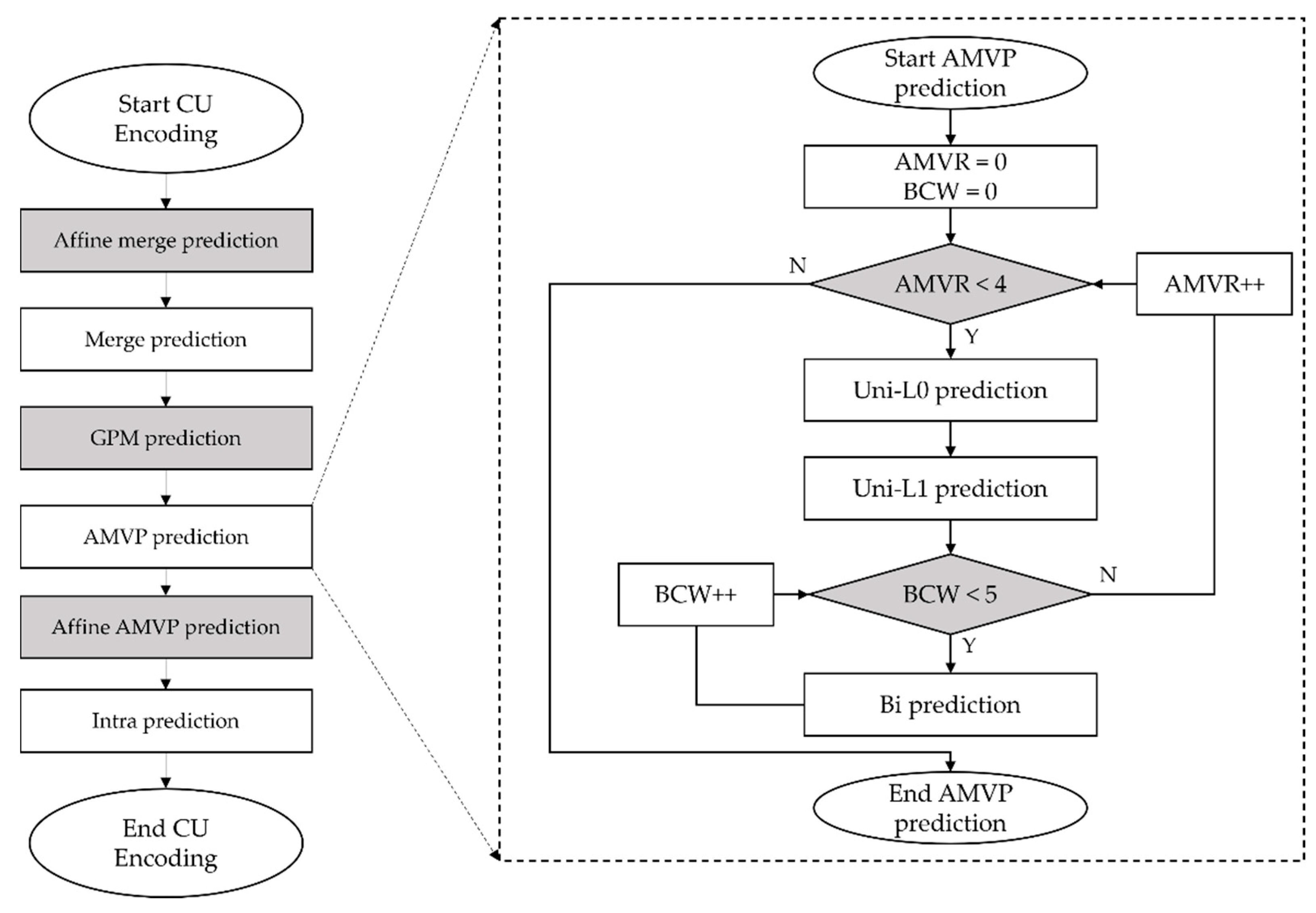
Figure 1 shows the CU encoding procedure in VVC. First, a CU performs the encoding process according to the order of affine merge, regular merge, GPM prediction, and AMVP prediction. In AMVP prediction, the five BCW weights are performed as the bi-prediction within the loop of the four AMVR iterations. Finally, the optimal mode of the current CU is determined after performing intra prediction.

Recently, several studies have aimed to reduce the computational complexity of VVC encoders. These studies mainly focused on reducing the complexity of the new block partitioning tools in VVC. In addition, studies utilizing convolutional neural networks (CNNs) or multilayer perceptrons (MLPs) for complexity reduction have showed convincing results from the development of deep learning technology. Zhao et al. [13] proposed the complexity reduction algorithm of VVC intra prediction based on statistical analysis and a size-adaptive CNN (SAE-CNN) to determine whether to split CUs of different sizes. Zhang et al. [14] designed a prediction tool using DenseNet to predict the probability of whether the edges of 4 × 4 CU units are division boundaries and consequently reduce the coding complexity of VVC. Yoon et al. [15] proposed an activity-based fast block partitioning decision method using the information of the current CU, minimizing the dependence on the QP and utilizing the gradient calculation used in the adaptive loop filter (ALF). Wang et al. [16] designed a multistage early termination CNN (MET-CNN) model to predict the partition information of 32 × 32-sized CUs. In addition, they proposed the concept of stage grid maps by dividing the entire partition into four stages to represent the structured output and consequently predict all partition information of the 32 × 32-sized CUs and their sub-CUs as the model outputs. Zhao et al. [17] proposed a support vector machine (SVM)-based fast CU partition decision algorithm by analyzing the ratio of the split modes of CUs of different sizes to effectively reduce the coding complexity of VVC. Jin et al. [18] proposed a CNN-based fast QTBT partitioning method to predict the depth range of the QTBT partition for 32 × 32 blocks based on the inherent texture richness of the image rather than judging the split at each depth level. Pan et al. [19] proposed an early termination of the QTMT-based block partition process using a multi-information fusion CNN (MFCNN) model. In addition, a content-complexity-based early merge mode decision method was proposed for the CU prediction residuals and the confidence of MFCNN. Liu et al. [20] designed a CNN-based model for fast inter partitioning in VVC, limiting the QT split search and avoiding partitions that are unlikely to be selected.

In VVC, complexity reduction studies of prediction tools were mainly conducted on statistical characteristics. Jung et al. [21] proposed a fast affine prediction method that determines whether to perform a context-based affine prediction mode to reduce inter-prediction complexity. Zhang et al. [22] proposed a fast GPM decision algorithm by comparing the average values of the gradients in four directions of the CUs to determine whether to perform GPM in VVC. They used the Sobel operator to calculate the gradients and determined six GPM candidate modes based on the gradient directions. Tun et al. [23] investigated the relationship between the RD cost and the sum of absolute transformed difference (SATD) of rough mode decision (RMD) to decrease the RDO calculations of intra-prediction modes. Park et al. [24] proposed a method to reduce the encoding complexity of intra prediction, which designed a light gradient boosting machine (LightGBM) model using the average absolute sum of transform coefficients as a key feature to determine whether to perform the ISP mode. Dong et al. [25] proposed a fast intra mode decision algorithm consisting of two aspects of mode selection and prediction termination. Shang et al. [26] also designed a fast intra-prediction algorithm based on statistical characteristics using the distribution of neighboring coding regions and prediction modes to skip unnecessary splits and prediction modes in advance. Although studies to reduce the complexity of intra-prediction tools have been conducted in various aspects, more studies are needed to speed up the newly adopted inter-prediction tools in VVC.

3. Proposed Method

To implement a fast encoding algorithm on the limited hardware platform, it is efficient to use an MLP with lower complexity than a CNN. Therefore, the proposed method designed an MLP-based neural network that exhibits significantly lower complexity than the CNN-based model.

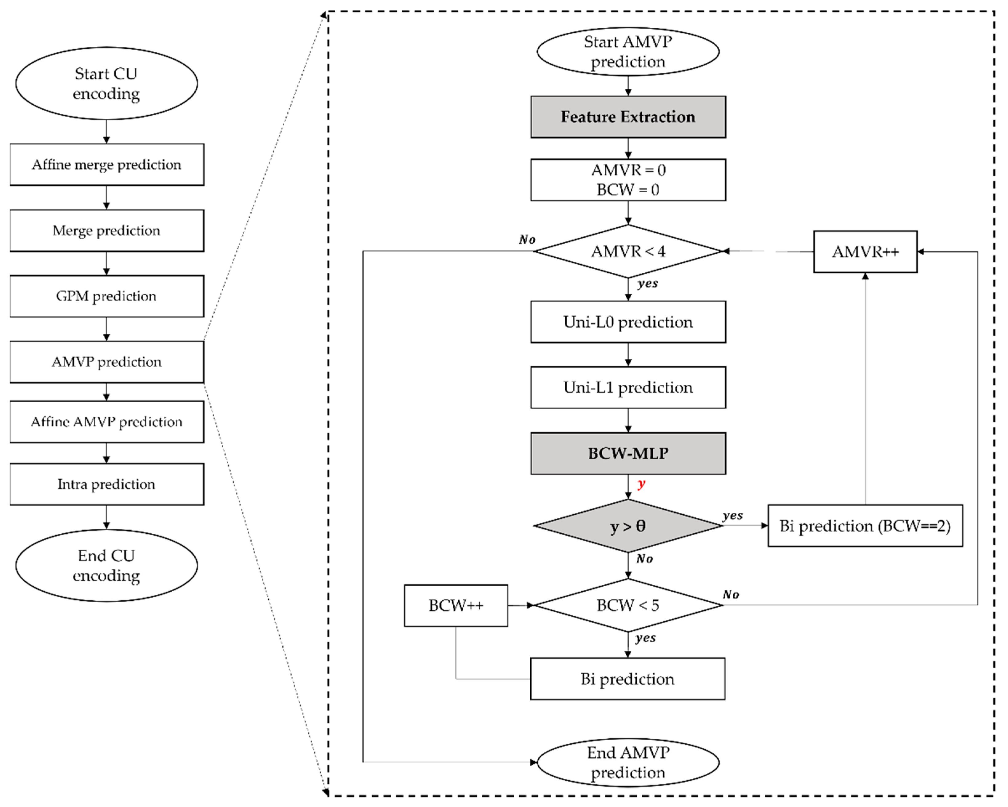
As shown in Figure 2, the proposed method is divided into two processes: extracting input features and determining whether to perform average weighting based on the output of the BCW-MLP. First, we extracted six input features to be fed into the BCW-MLP model. Subsequently, the BCW-MLP model outputted the y value to determine whether to perform the BCW with average weight. If the output y value is greater than the predefined threshold, the BCW-Idx 2 is performed; otherwise, the encoding process is performed for all BCW modes.

3.1. Feature Extraction for BCW-MLP

In this study, the proposed method defined the relationship between the parent and neighboring CUs of a current CU, where the parent CU can be a square QT node or a rectangular MTT node covering the area of the current CU. On the other hand, the neighboring CUs refer to the left and above CUs, which complete the encoding and decoding process.

The network input features are classified into four categories, all input features are extracted during the encoding process, and each input feature is converted into a value between 0 and 1. The first category shows the correlation of the BCW modes with the parent and neighboring CUs, which can be related to the current BCW mode. The second category includes base QP, slice QP, and temporal layers, which are features associated with QP. The third category represents the current CU size, such as width, height, and pixel ratios. Finally, the fourth category consists of AMVR and coded block flags (CBFs), which are related to the interference of other prediction tools.

Table 3. Description of input feature candidates per category.

Category	Features	Description
BCW Mode	Parent BCW	BCW mode derived from parent CU is divided by 6.
	Neighboring BCW	If the BCW mode derived from the left CU has an average weight, the value is increased by 0.5. Similarly, if the BCW mode derived from the above CU has an average weight, the value is increased by 0.5.
QP	Base QP	Base QP is divided by 63.
	Slice QP	Slice QP is divided by 63.
	Temporal Layer	Temporal layer is divided by 5.
Block Size	Width Ratio	W/(W + H) 1
	Height Ratio	H/(H + W)
	Pixel Ratio	W × H/128 × 128
Prediction	AMVR	AMVR mode is divided by 4.
	CBF	Coded block flag value is divided by 3.

¹ W and H are the width and height of the current CU, respectively.

presents the detailed definitions of the abovementioned input feature candidates.

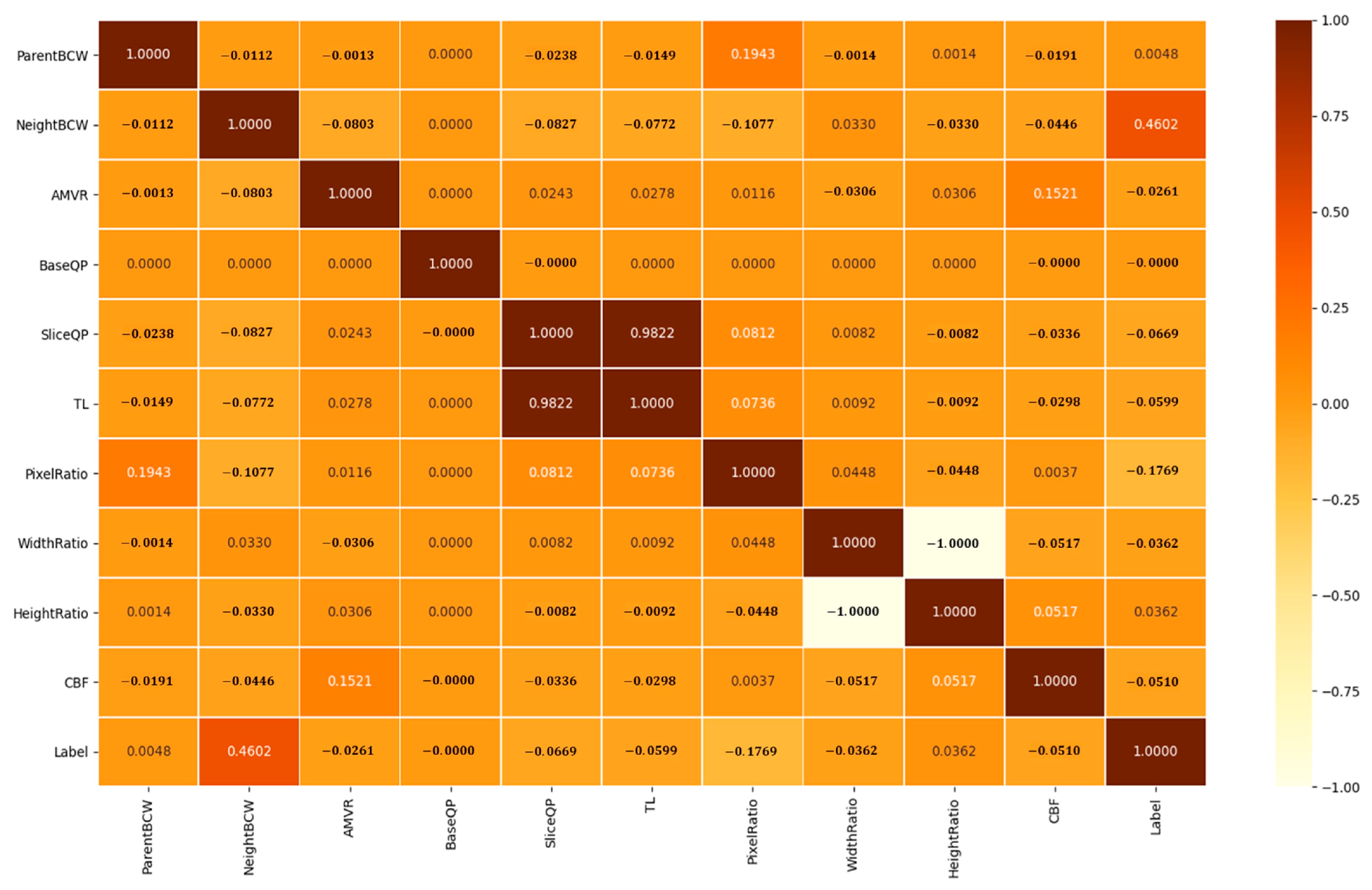
The proposed BCW-MLP model selects fewer input feature candidates to set the input features based on a Pearson correlation coefficient (PCC) heatmap between the input feature candidates and labels as illustrated in Figure 3. In the first category of Table 3, two input feature candidates were selected as input features, because they have a strong relationship with the current BCW mode. In the second category of Table 3, the slice QP has a higher correlation with the label than the base QP and the temporal layer (TL). Additionally, strong intercorrelations exist among features, for example, the PCC between the slice QP and TL was 0.9822. The pixel ratio with the highest correlation in the third category was set as the input feature. Finally, we used two candidates as input features in the fourth category. Therefore, six candidates were used as input features to design the BCW-MLP model, which are parent BCW, neighboring BCW, slice QP, pixel ratio, AMVR, and CBF, respectively.

3.2. Fast Mode Decision Algorithm Using BCW-MLP

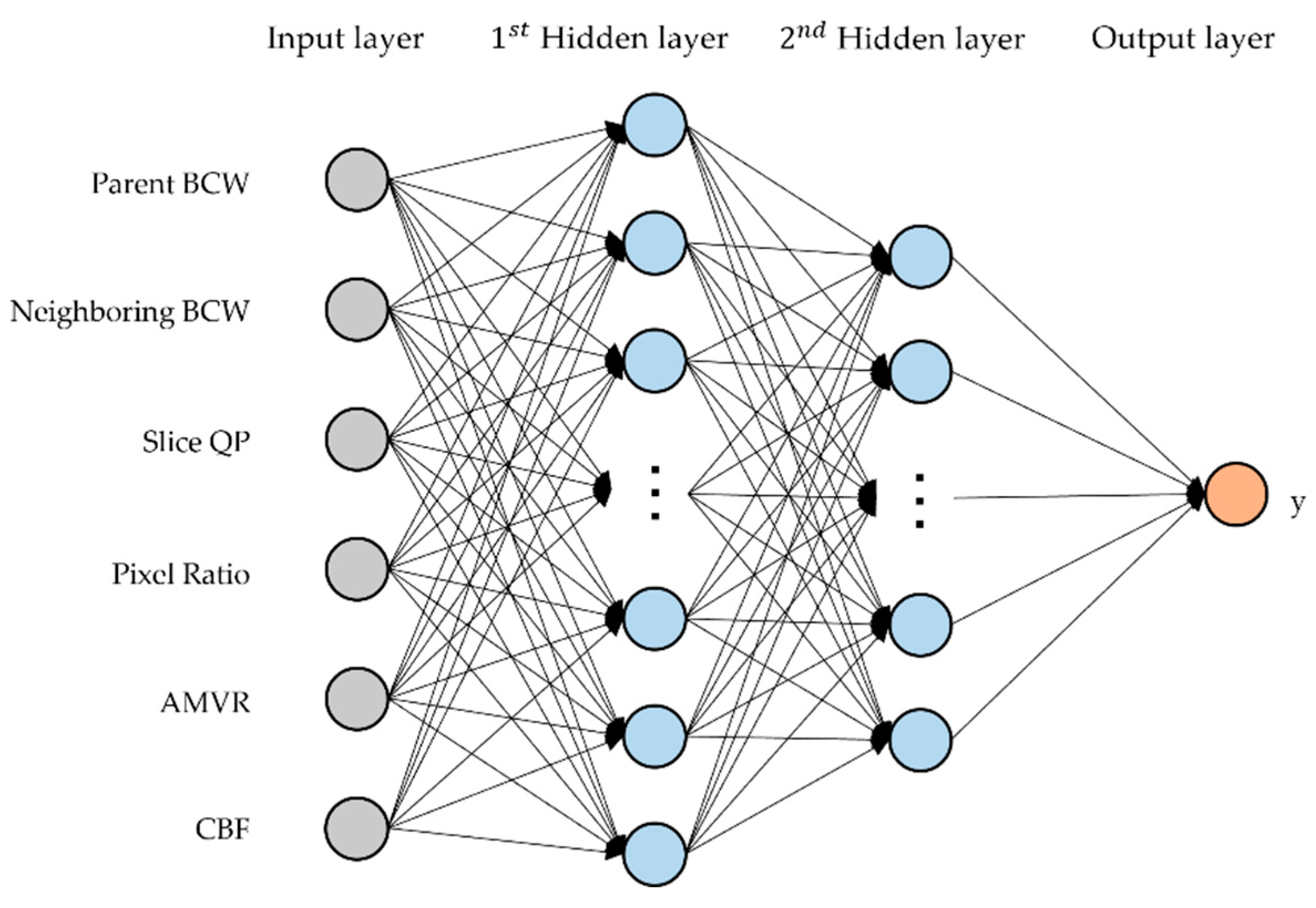
We implemented an MLP architecture before the BCW mode, defined as BCW-MLP, to determine whether to perform the BCW mode—except for the average-weight BCW mode. In the feature extraction stage, a one-dimensional (1D) column vector with six input features was generated as the input vector of BCW-MLP. As shown in Figure 4, the BCW-MLP consists of six input nodes, two hidden layers with 30 and 15 hidden nodes, and one output node, respectively.

The output of the $j$th neuron is calculated as in Equation (2):

$$y_j=f\left(\sum {\stackrel{-}{w}}_{ji}{\stackrel{-}{x}}_i+b_j\right),where j=1,\dots ,\phi$$

(2)

where ${\stackrel{-}{x}}_i$, ${\stackrel{-}{w}}_{ji}$, $b_j$, and $\phi$ denote the $i$th input feature, the filter weight corresponding to the $i$th input feature, the bias value of the $j$th node, and the number of nodes within each layer, respectively. In addition, $f\left(·\right)$ indicates activation functions of the hidden layer and output layer, which are ReLU and sigmoid function, respectively, and $y_j$ denotes the output of $f\left(·\right)$ the $j$th neuron. The network output $y$ has a value between 0 and 1. Note that when the output values of the model are close to 1, then only the average-weight BCW mode is performed among the BCW modes.

To establish an appropriate threshold, we investigated the ratio of average weighted BCW modes to the output values of the network.

Table 4. Ratio of BCW mode according to output value.

Output Range	Ratio of BCW Mode
	Average Weight	Other Weight
0.0~0.1	72%	28%
0.1~0.2	78%	22%
0.2~0.3	72%	28%
0.3~0.4	76%	24%
0.4~0.5	54%	46%
0.5~0.6	83%	17%
0.6~0.7	92%	8%
0.7~0.8	92%	8%
0.8~0.9	75%	25%
0.9~1.0	94%	6%

describes the ratio of optimal BCW modes determined by the RDO process during encoding and the distribution by the range of network output values. It can be observed that when the network output value was 0.6 or higher, the distribution of the average weighted BCW mode was over 90%. In this paper, the threshold was set to 0.6. Then, the encoder performs only the average-weight BCW mode when the output value is larger than the threshold.

4. Experimental Results

The proposed method was implemented on top of VTM-11.0 using the Keras2.2.4 library on Python 3.6.8.

Table 5. Training environments of the proposed network.

Settings	Options
Training Sequence	BVI-DVC
Number of Sequences	12
Resolution	3840 × 2160
Number of Datasets	12,511,937
Quantization Parameters	22, 32
Framework	Keras2.2.4

shows the training environments of the proposed network. The proposed network was trained using the BVI-DVC dataset [27] with a resolution of 3840 × 2160 pixels and the QPs were set to 22 and 32. The size of the training dataset is 12,511,937 images, which were collected from various CU sizes during the encoding process. In addition, 20% of the data were used as the validation set.

Table 6. Hyperparameters of the proposed network.

Hyperparameters	Options
Optimizer	Adam
Activation Function	ReLU, Sigmoid
Loss Function	Mean Squared Error
Learning Rate	0.01
Number of Epochs	100
Batch Size	512
Dataset Sampling	Random Undersampling
Initial Weight	Xavier

lists the hyperparameters used to train the proposed network. While the activation function of all hidden layers, except the final output layer, was set to ReLU, the output layer used the sigmoid function to compute a floating value between 0 and 1. The batch size, learning rate, and optimization method were set to 512, 0.01, and stochastic gradient descent (SGD) [28], respectively. 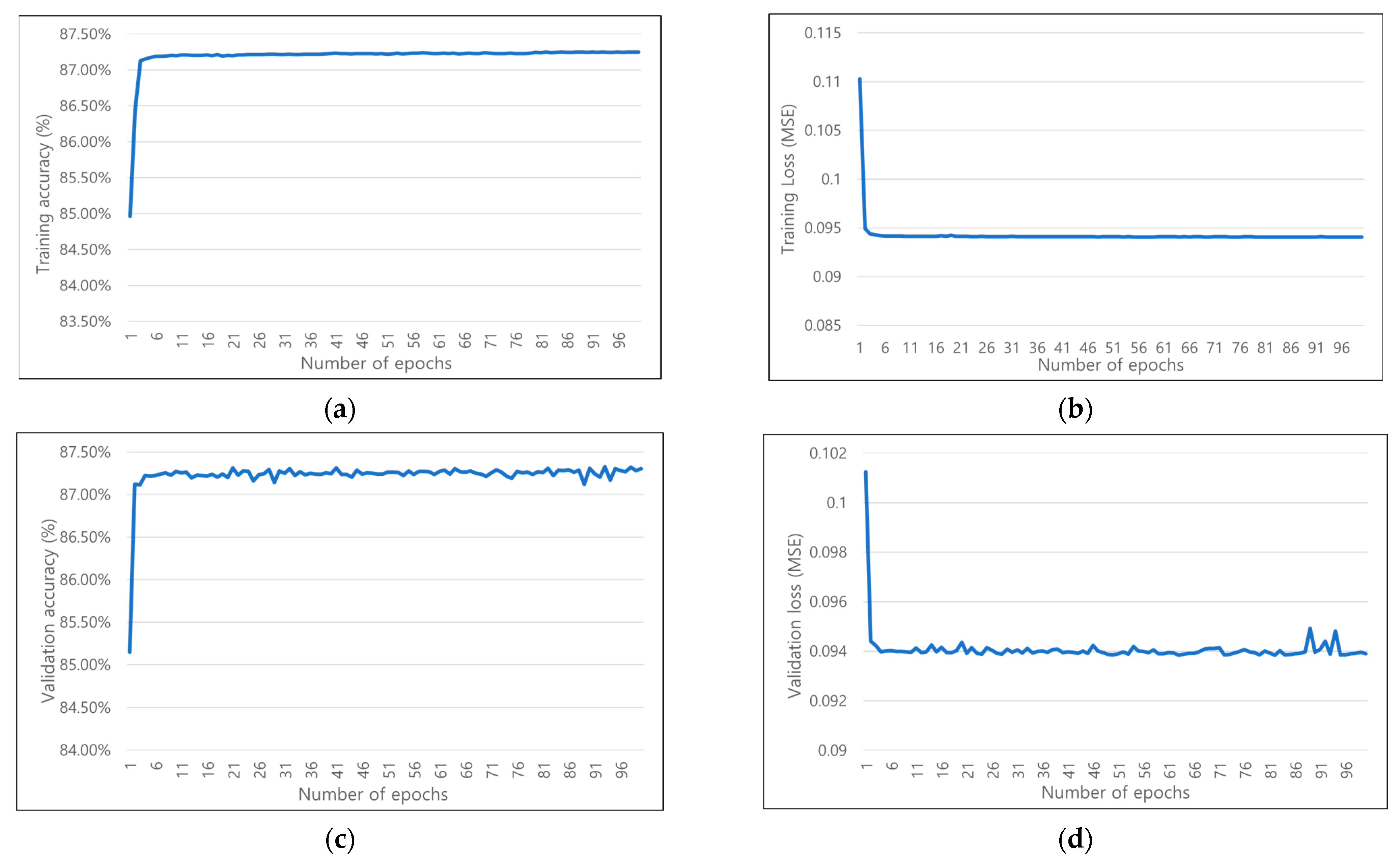The weight initialization of the hidden layers was performed according to Xavier’s normalized initialization procedure [29], whereby the optimized model parameters were updated iteratively within a predefined epoch number and the Mean Squared Error (MSE) was used as a loss function.

Figure 5 shows the training and validation results of the proposed network, which measure the accuracy of the optimal BCW mode and loss functions according to the number of epochs.

To investigate the optimal architecture of BCW-MLP, various ablation works were conducted in terms of the number of input features, hidden layers, and nodes per hidden layer as shown in

Table 7. Ablation works of the proposed BCW-MLP.

Network	Training		Validation		Network	Training		Validation
	Loss	Accuracy	Loss	Accuracy		Loss	Accuracy	Loss	Accuracy
6 × 15 × 1	0.0955	0.8699	0.0957	0.8694	6 × 45 × 15 × 1	0.0941	0.8724	0.0942	0.8724
6 × 30 × 1	0.0940	0.8722	0.0940	0.8721	6 × 45 × 30 × 1	0.0941	0.8720	0.0945	0.8725
6 × 45 × 1	0.0941	0.8722	0.0940	0.8721	6 × 45 × 45 × 1	0.0941	0.8723	0.0942	0.8718
6 × 60 × 1	0.0940	0.8722	0.0941	0.8723	6 × 45 × 60 × 1	0.0941	0.8718	0.0945	0.8716
6 × 75 × 1	0.0941	0.8722	0.0941	0.8723	6 × 45 × 75 × 1	0.0942	0.8719	0.0944	0.8720
6 × 15 × 15 × 1	0.0941	0.8722	0.0938	0.8727	6 × 60 × 15 × 1	0.0941	0.8723	0.0940	0.8724
6 × 15 × 30 × 1	0.0942	0.8719	0.0940	0.8725	6 × 60 × 30 × 1	0.0942	0.8720	0.0943	0.8721
6 × 15 × 45 × 1	0.0942	0.8721	0.0941	0.8725	6 × 60 × 45 × 1	0.0942	0.8721	0.0944	0.8712
6 × 15 × 60 × 1	0.0941	0.8724	0.0939	0.8726	6 × 60 × 60 × 1	0.0941	0.8724	0.0940	0.8729
6 × 15 × 75 × 1	0.0941	0.8721	0.0941	0.8722	6 × 60 × 75 × 1	0.0942	0.8720	0.0939	0.8722
6 × 30 × 15 × 1	0.0940	0.8730	0.0940	0.8730	6 × 75 × 15 × 1	0.0942	0.8719	0.0940	0.8725
6 × 30 × 30 × 1	0.0947	0.8715	0.0944	0.8720	6 × 75 × 30 × 1	0.0941	0.8724	0.0939	0.8728
6 × 30 × 45 × 1	0.0939	0.8726	0.0943	0.8719	6 × 75 × 45 × 1	0.0942	0.8719	0.0941	0.8712
6 × 30 × 60 × 1	0.0943	0.8716	0.0943	0.8719	6 × 75 × 60 × 1	0.0941	0.8721	0.0939	0.8727
6 × 30 × 75 × 1	0.0941	0.8721	0.0940	0.8724	6 × 75 × 75 × 1	0.0940	0.8724	0.0941	0.8720

. After considering both the accuracy and the loss of networks, BCW-MLP has two hidden layers with 30 and 15 nodes in the first and second layer, respectively.

In addition, tool-off tests on the validation and training datasets were performed to measure the effectiveness of the six input features.

Table 8. Tool-off tests among the input features.

Network	Training		Validation
	Loss	Accuracy	Loss	Accuracy
All Features	0.0941	0.8725	0.0939	0.8730
Tool-off of Parent BCW	0.0970	0.8689	0.0971	0.8693
Tool-off of Neighboring BCW	0.1548	0.7628	0.1547	0.7634
Tool-off of SliceQP	0.0952	0.8698	0.0950	0.8705
Tool-off of PixelRatio	0.1376	0.8140	0.1376	0.8142
Tool-off of AMVR	0.0956	0.8701	0.0954	0.8705
Tool-off of CBF	0.0942	0.8718	0.0940	0.8717

represents the experimental results obtained by omitting one of the six input features and shows that each input feature has an effect on the performance of our network. In particular, the neighboring BCW is observed as the most effective input feature of BCW-MLP.

All experiments were run on an Intel Xeon Gold 6230R 52-cores 2.10 GHz processor with 256 GB RAM operated by the 64-bit Windows server 2019. In class A (3840 × 2160) and B (1920 × 1080) sequences of JVET CTC, the performance of the proposed method was evaluated under the random-access (RA) and the low-delay-B (LDB) configuration and compared with VTM-11.0. Additionally, the trained model was converted to the C++ standard format and implemented in the VTM-11.0. To measure the coding loss, we used the Bjontegaard Delta Bit Rate (BDBR) [30]. In general, a BDBR increase of 1% corresponds to a BD-PSNR decrease of 0.05 dB, where the positive increment in BDBR indicates coding loss. The weighted averages of the BDBR of the Y, U, and V color components were measured as in Equation (3):

$${BDBR}_{YUV}=\frac{6\times {BDBR}_Y+{BDBR}_U+{BDBR}_V}{8}$$

(3)

where ${BDBR}_Y$, ${BDBR}_U$, and ${BDBR}_V$ denote the BDBRs of the Y, U, and V color components, respectively. To evaluate the encoding time (ET) reduction, the ${ET}_{tool\_off}$ and ${ET}_{proposed}$ are computed as in Equations (4) and (5):

$${ET}_{tool\_off}=\frac{1}{4}\sum _{{QP}_i\in \left\{\mathrm{22,27,32,37}\right\}}\frac{T_{org}\left({QP}_i\right)-T_{tool\_off}\left({QP}_i\right)}{T_{org}\left({QP}_i\right)}$$

(4)

$${ET}_{proposed}=\frac{1}{4}\sum _{{QP}_i\in \left\{\mathrm{22,27,32,37}\right\}}\frac{T_{org}\left({QP}_i\right)-T_{proposed}\left({QP}_i\right)}{T_{org}\left({QP}_i\right)}$$

(5)

where $T_{org}$, $T_{tool\_off}$, and $T_{proposed}$ indicate the total encoding times of the anchor, tool-off test, and proposed methods, respectively. For comparison of the computational complexities, we measured the time savings of total encoding time (TET) and BCW encoding time (BET) by Equations (6) and (7):

$$TET=\frac{{TET}_{tool\_off}-{TET}_{proposed}}{{TET}_{tool\_off}}$$

(6)

$$BET=\frac{{BET}_{tool\_off}-{BET}_{proposed}}{{BET}_{tool\_off}}$$

(7)

where ${TET}_{tool\_off}$, ${TET}_{proposed}$, ${BET}_{tool\_off}$, and ${BET}_{proposed}$ mean the TET of the ${ET}_{tool\_off}$, TET of the ${ET}_{proposed}$, BET of the ${ET}_{tool\_off}$, and BET of the ${ET}_{proposed}$, respectively. For reference, BET measures the time taken only for the portion of the VVC encoder process that performs bi-prediction. In summary, the performance comparisons between the proposed method and the anchor are presented in

Table 9. Coding performance of proposed method over VTM-11.0 under the RA configuration.

Class	Sequences	${\mathit{B}\mathit{D}\mathit{B}\mathit{R}}_{\mathit{Y}}$	${\mathit{B}\mathit{D}\mathit{B}\mathit{R}}_{\mathit{U}}$	${\mathit{B}\mathit{D}\mathit{B}\mathit{R}}_{\mathit{V}}$	${\mathit{B}\mathit{D}\mathit{B}\mathit{R}}_{\mathit{Y}\mathit{U}\mathit{V}}$	TET	BET
A	Tango2	0.25%	0.47%	0.43%	0.30%	41%	39%
	FoodMarket4	0.24%	0.38%	0.48%	0.29%	51%	39%
	CatRobot	0.36%	0.50%	0.46%	0.39%	22%	15%
	DaylightRoad2	0.05%	0.39%	0.09%	0.10%	28%	33%
	Average	0.23%	0.43%	0.36%	0.27%	35%	32%
B	MarketPlace	0.19%	0.62%	0.08%	0.23%	23%	37%
	RitualDance	0.28%	0.15%	0.22%	0.26%	25%	37%
	Cactus	0.14%	0.07%	0.10%	0.12%	26%	18%
	BasketballDrive	0.36%	0.41%	0.18%	0.34%	55%	47%
	BQTerrace	0.33%	0.21%	0.14%	0.29%	21%	33%
	Average	0.26%	0.29%	0.15%	0.25%	30%	34%
Total Average		0.24%	0.35%	0.24%	0.26%	32%	33%

. Compared to the anchor, the proposed method can achieve average time savings of 32% and 33% in terms of TET and BET, respectively.

Table 10. Coding performance of proposed method over VTM-11.0 under the LDB configuration.

Class	Sequences	${\mathit{B}\mathit{D}\mathit{B}\mathit{R}}_{\mathit{Y}}$	${\mathit{B}\mathit{D}\mathit{B}\mathit{R}}_{\mathit{U}}$	${\mathit{B}\mathit{D}\mathit{B}\mathit{R}}_{\mathit{V}}$	${\mathit{B}\mathit{D}\mathit{B}\mathit{R}}_{\mathit{Y}\mathit{U}\mathit{V}}$	TET	BET
B	MarketPlace	−0.10%	−0.46%	−0.45%	−0.19%	44%	58%
	RitualDance	−0.02%	−0.05%	−0.28%	−0.06%	21%	30%
	Cactus	0.11%	0.20%	0.34%	0.15%	44%	62%
	BasketballDrive	0.04%	−0.10%	0.16%	0.04%	9%	33%
	BQTerrace	0.27%	0.46%	0.95%	0.38%	54%	64%
Average		0.06%	0.01%	0.14%	0.06%	35%	49%

shows the performance comparisons between the proposed method and the anchor under the LDB configuration. In addition, the proposed method was tested for class B. Compared to the anchor, the proposed method achieved average time savings of 35% and 49% in terms of TET and BET, respectively. The experimental results show that the proposed method achieves higher coding efficiency in the LDB configuration compared to the RA configuration.

5. Conclusions

VVC has newly adopted the BCW method to enhance conventional bi-prediction. It was possible to improve the coding performance compared to conventional bi-prediction, but it caused high encoding complexity. In this study, the complexity reduction in BCW was addressed with the decision rule of BCW-MLP. We proposed a fast BCW mode decision method using a lightweight MLP to determine whether to perform the BCW mode—except for the average-weight BCW mode. The proposed BCW-MLP consists of six input nodes, two hidden layers with 30 and 15 nodes, and one output node. To reduce the encoding complexity of BCW and minimize coding loss, six input features were investigated by analyzing the correlation between the input features. In addition, various verification tests were conducted to determine the optimal network architecture. The proposed method was evaluated under the JVET CTC and compared with VTM-11.0 as an anchor. Our experimental results show reductions in the average encoding complexity of 32% and 35%, with unnoticeable coding loss compared to the anchor of RA and LDB, respectively.