
Visual Explanations of Deep Learning Architectures in Predicting Cyclic Alternating Patterns Using Wavelet Transforms

 , ,
, ,  , and
, and
Abstract
:1. Introduction
2. Methods
2.1. Dataset
2.2. Pre-Processing
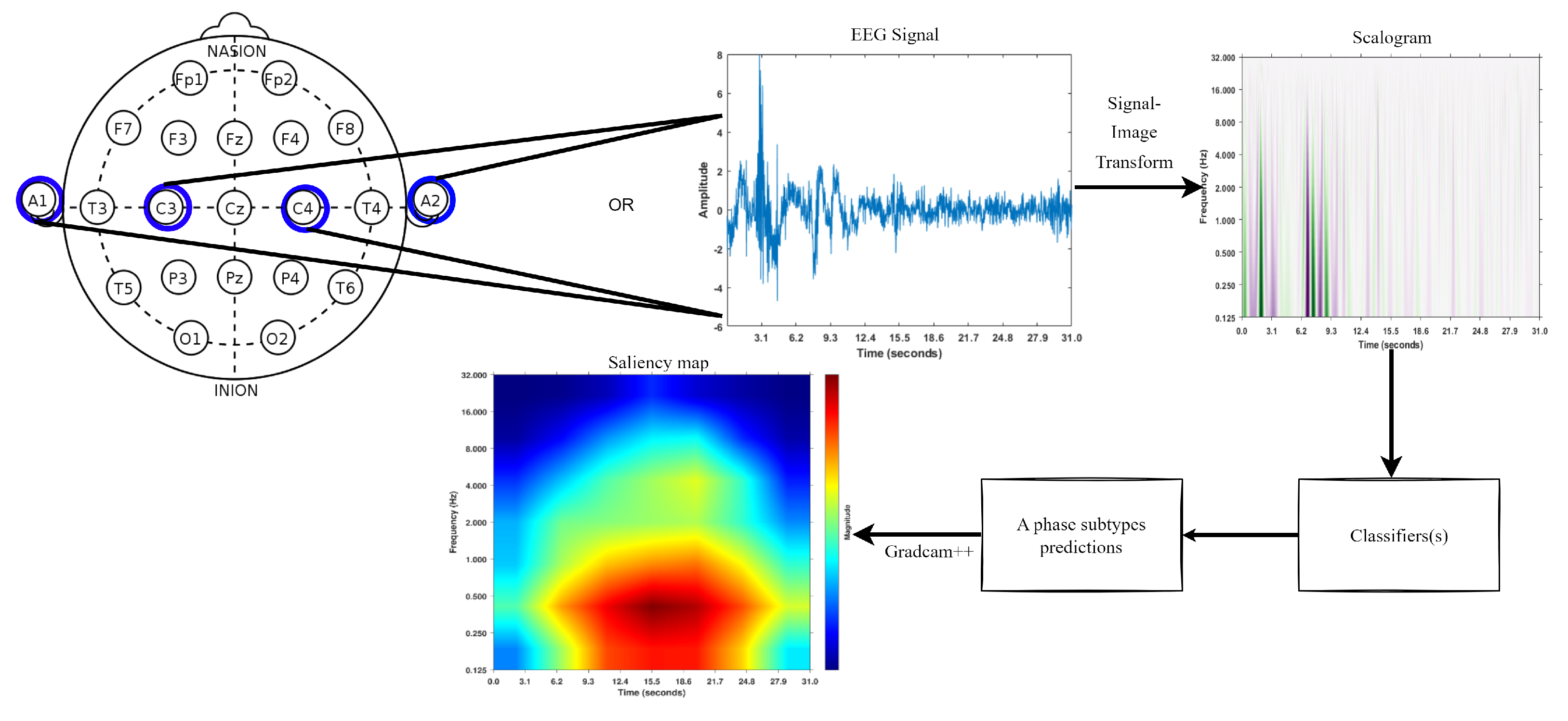
2.3. Signal to Image Conversion
2.4. Deep Learning Models
2.4.1. Training Parameters
2.4.2. VGG19
2.4.3. ResNet50
2.4.4. InceptionNetV3
2.4.5. Densenet121
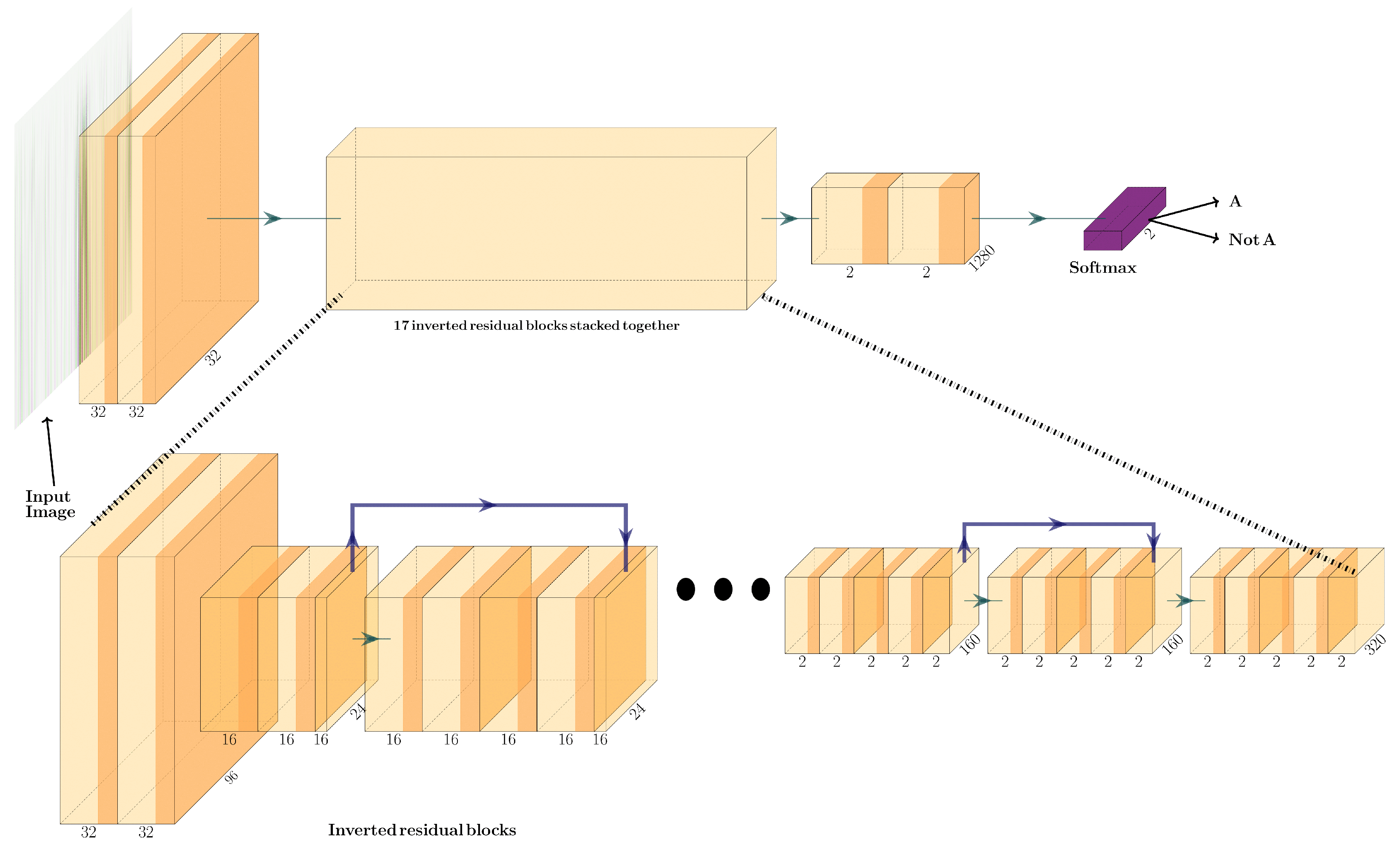
2.4.6. MobileNetV2
2.4.7. EfficientNetB0
2.5. Understanding the Classifier Decisions
3. Results
3.1. Signal to Scalogram Transformation
3.2. Parameters and Data Splitting
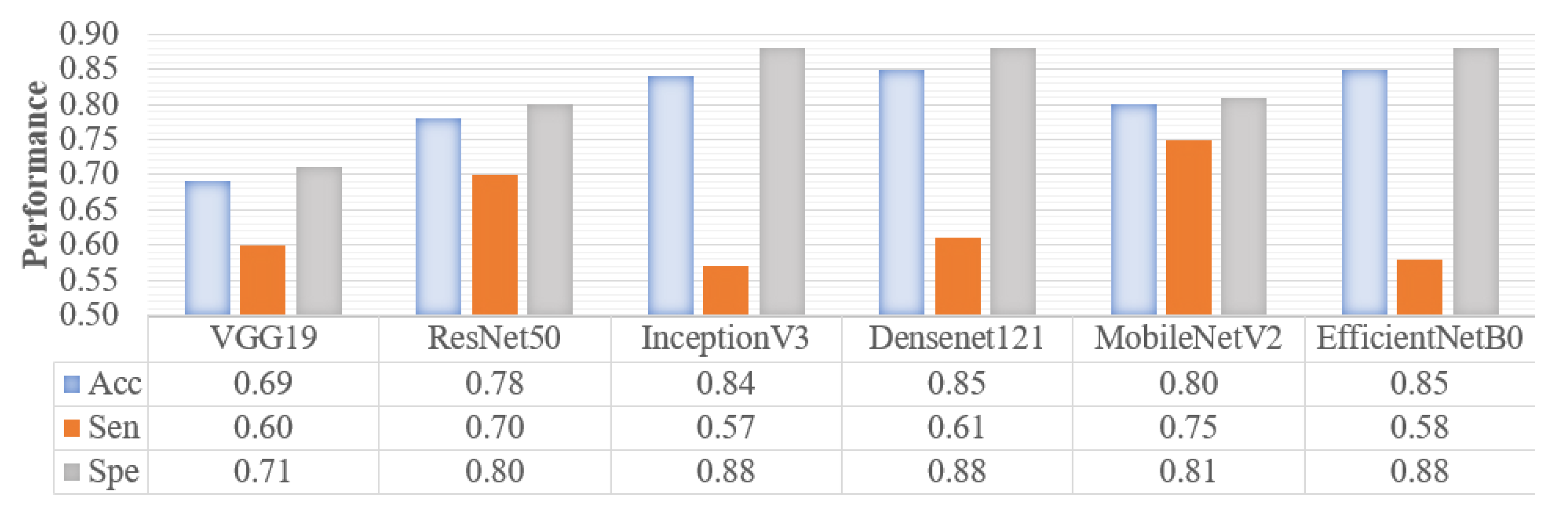
3.3. Performance Analysis
3.3.1. A/Not-A-Phase Prediction
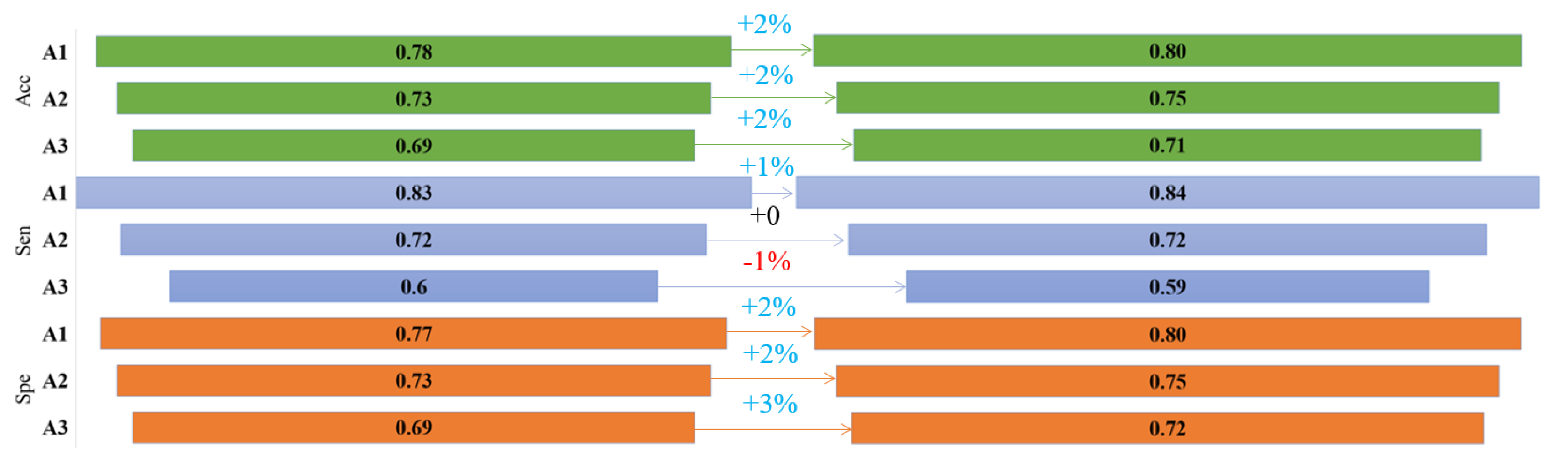
3.3.2. A-Subtypes Classification
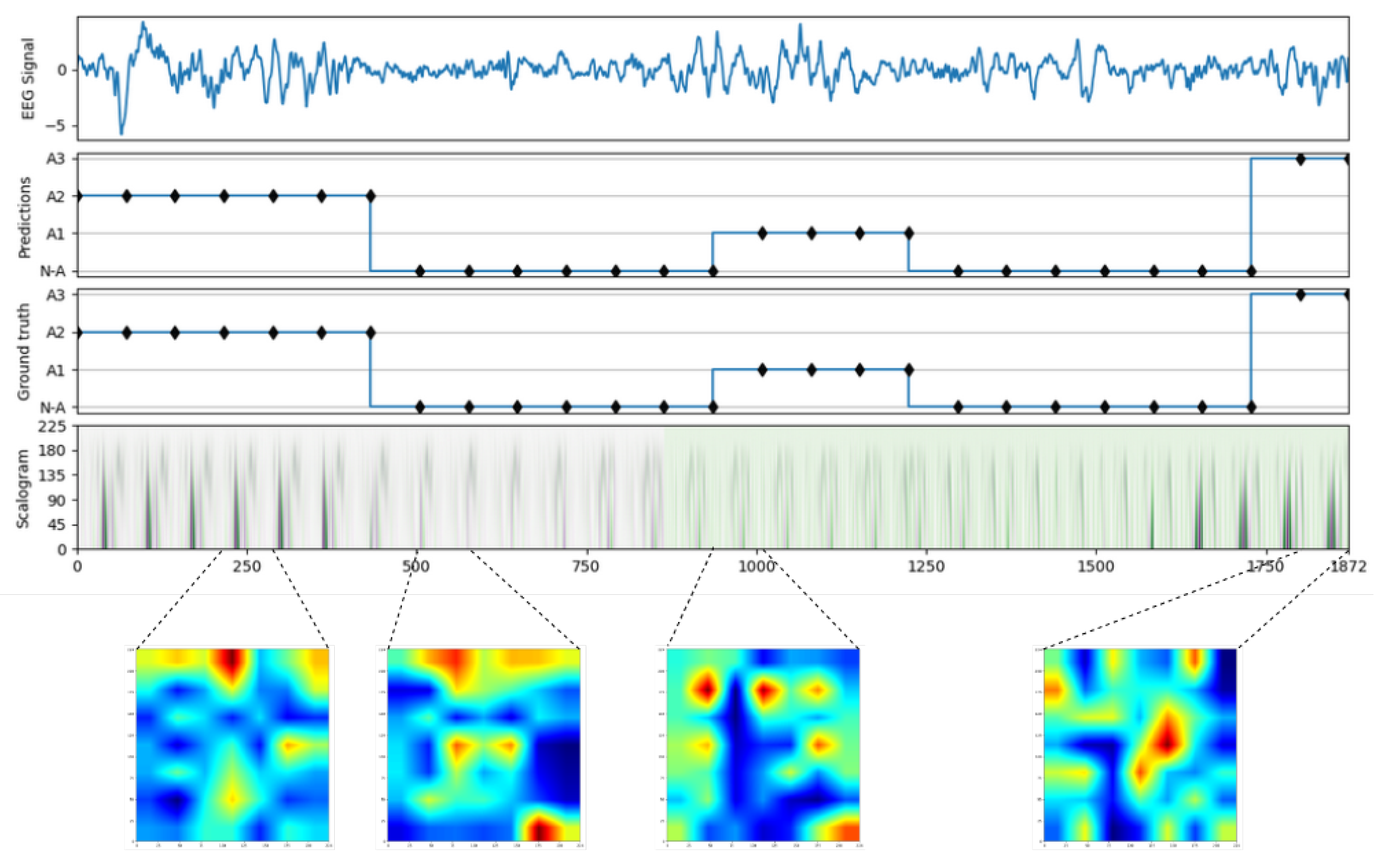
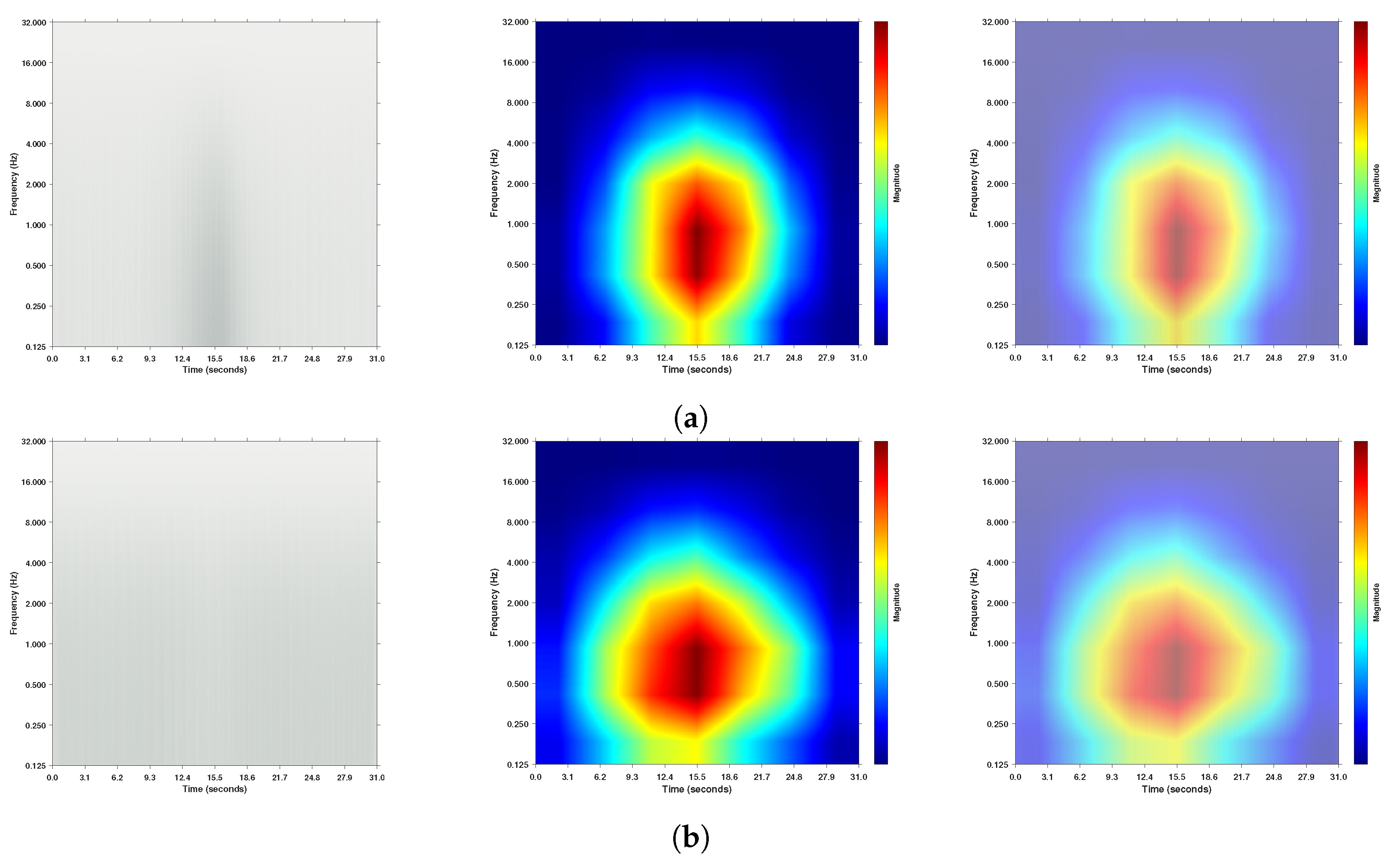
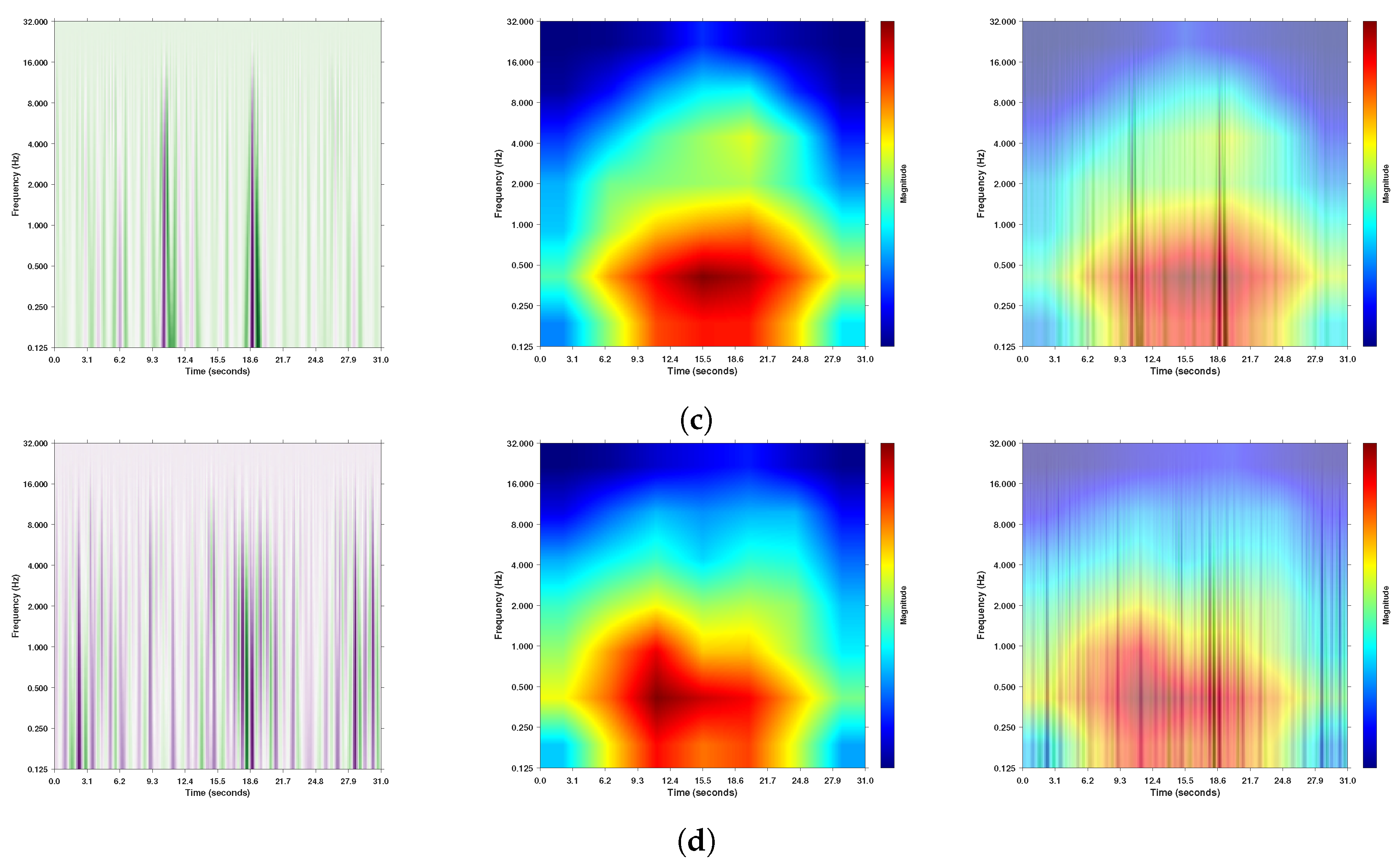
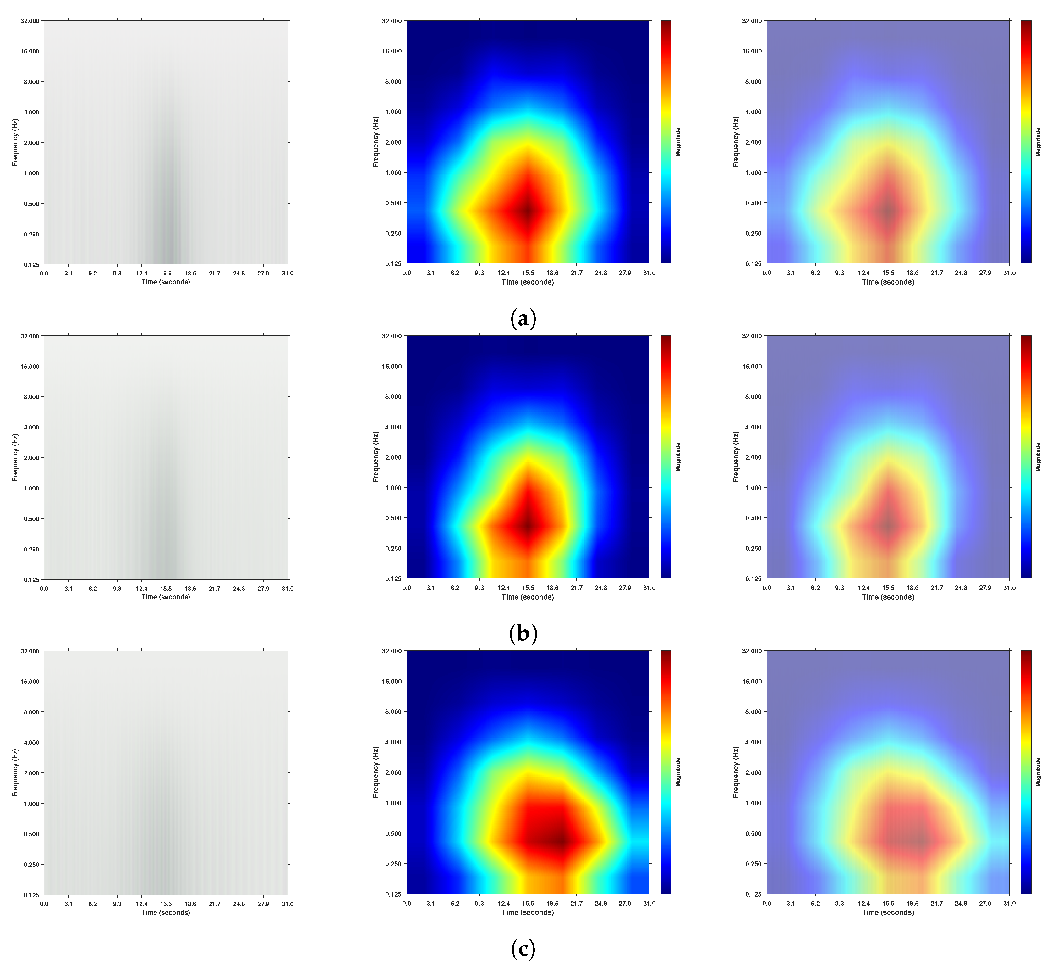
3.4. Visualizing the Regions Targeted Using Gradcam++
3.4.1. Binary Classification A/Not-A-Phase Classification
3.4.2. A-Phase Subtype Classification
4. Discussion
5. Conclusions
Author Contributions
Funding
Institutional Review Board Statement
Informed Consent Statement
Data Availability Statement
Acknowledgments
Conflicts of Interest
References
- Berry, R.B.; Brooks, R.; Gamaldo, C.; Harding, S.M.; Lloyd, R.M.; Quan, S.F.; Troester, M.T.; Vaughn, B.V. AASM scoring manual updates for 2017 (version 2.4). J. Clin. Sleep Med. 2017, 13, 665–666. [Google Scholar] [CrossRef] [PubMed]
- Terzano, M.G.; Parrino, L.; Smerieri, A.; Chervin, R.; Chokroverty, S.; Guilleminault, C.; Hirshkowitz, M.; Mahowald, M.; Moldofsky, H.; Rosa, A.; et al. Atlas, rules, and recording techniques for the scoring of cyclic alternating pattern (CAP) in human sleep. Sleep Med. 2002, 3, 187–199. [Google Scholar] [CrossRef] [PubMed]
- Terzano, M.G.; Parrino, L. Origin and significance of the cyclic alternating pattern (CAP). Sleep Med. Rev. 2000, 4, 101–123. [Google Scholar] [CrossRef] [PubMed]
- Yeh, C.H.; Shi, W. Identifying phase-amplitude coupling in cyclic alternating pattern using masking signals. Sci. Rep. 2018, 8, 2649. [Google Scholar] [CrossRef] [PubMed] [Green Version]
- Medina-Ibarra, D.; Mendez, M.O.; Chouvarda, I.; Murguía, J.; Alba, A.; Arce-Santana, E.R.; Bianchi, A. Assessment of Singularities in the EEG during A-phases of Sleep based on Wavelet Decomposition. IEEE Trans. Neural Syst. Rehabil. Eng. 2022, 30, 2721–2731. [Google Scholar] [CrossRef] [PubMed]
- Parrino, L.; Ferri, R.; Bruni, O.; Terzano, M.G. Cyclic alternating pattern (CAP): The marker of sleep instability. Sleep Med. Rev. 2012, 16, 27–45. [Google Scholar] [CrossRef]
- Terzano, M.G.; Parrino, L. Clinical applications of cyclic alternating pattern. Physiol. Behav. 1993, 54, 807–813. [Google Scholar] [CrossRef]
- Rosa, A.; Alves, G.R.; Brito, M.; Lopes, M.C.; Tufik, S. Visual and automatic cyclic alternating pattern (CAP) scoring. Arq. Neuro-Psiquiatr. 2006, 64, 578–581. [Google Scholar] [CrossRef] [Green Version]
- Chattopadhay, A.; Sarkar, A.; Howlader, P.; Balasubramanian, V.N. Grad-cam++: Generalized gradient-based visual explanations for deep convolutional networks. In Proceedings of the 2018 IEEE Winter Conference on Applications of Computer Vision (WACV), Lake Tahoe, NV, USA, 12–15 March 2018; pp. 839–847. [Google Scholar]
- Arino, M.A.; Morettin, P.A.; Vidakovic, B. Wavelet scalograms and their applications in economic time series. Braz. J. Probab. Stat. 2004, 18, 37–51. [Google Scholar]
- Byeon, Y.H.; Pan, S.B.; Kwak, K.C. Intelligent deep models based on scalograms of electrocardiogram signals for biometrics. Sensors 2019, 19, 935. [Google Scholar] [CrossRef] [Green Version]
- Türk, Ö.; Özerdem, M.S. Epilepsy detection by using scalogram based convolutional neural network from EEG signals. Brain Sci. 2019, 9, 115. [Google Scholar] [CrossRef] [Green Version]
- Kumar, J.L.M.; Rashid, M.; Musa, R.M.; Razman, M.A.M.; Sulaiman, N.; Jailani, R.; Majeed, A.P.A. The classification of EEG-based winking signals: A transfer learning and random forest pipeline. PeerJ 2021, 9, e11182. [Google Scholar] [CrossRef]
- Voulodimos, A.; Doulamis, N.; Doulamis, A.; Protopapadakis, E. Deep learning for computer vision: A brief review. Comput. Intell. Neurosci. 2018, 2018, 7068349. [Google Scholar] [CrossRef]
- Ling, C.X.; Sheng, V.S. Cost-sensitive learning and the class imbalance problem. Encycl. Mach. Learn. 2008, 2011, 231–235. [Google Scholar]
- Weinstein, C.J. Programs for digital signal processing. Proc. IEEE 1979, 69, 856–857. [Google Scholar]
- Hartmann, S.; Baumert, M. Automatic a-phase detection of cyclic alternating patterns in sleep using dynamic temporal information. IEEE Trans. Neural Syst. Rehabil. Eng. 2019, 27, 1695–1703. [Google Scholar] [CrossRef]
- Hatipoglu, B.; Yilmaz, C.M.; Kose, C. A signal-to-image transformation approach for eeg and meg signal classification. Signal Image Video Process. 2019, 13, 483–490. [Google Scholar] [CrossRef]
- Sadowsky, J. Investigation of signal characteristics using the continuous wavelet transform. Johns Hopkins Apl Tech. Dig. 1996, 17, 258–269. [Google Scholar]
- Wang, Y. Frequencies of the Ricker wavelet. Geophysics 2015, 80, A31–A37. [Google Scholar] [CrossRef] [Green Version]
- Bahg, G.; Evans, D.G.; Galdo, M.; Turner, B.M. Gaussian process linking functions for mind, brain, and behavior. Natl. Acad. Sci. 2020, 117, 29398–29406. [Google Scholar] [CrossRef]
- Arefnezhad, S.; Eichberger, A.; Frühwirth, M.; Kaufmann, C.; Moser, M.; Koglbauer, I.V. Driver monitoring of automated vehicles by classification of driver drowsiness using a deep convolutional neural network trained by scalograms of ECG signals. Energies 2022, 15, 480. [Google Scholar] [CrossRef]
- Simonyan, K.; Zisserman, A. Very deep convolutional networks for large-scale image recognition. arXiv 2014, arXiv:1409.1556. [Google Scholar]
- He, K.; Zhang, X.; Ren, S.; Sun, J. Deep residual learning for image recognition. In Proceedings of the IEEE Conference on Computer Vision and Pattern Recognition, Las Vegas, NV, USA, 27–30 June 2016; pp. 770–778. [Google Scholar]
- Szegedy, C.; Vanhoucke, V.; Ioffe, S.; Shlens, J.; Wojna, Z. Rethinking the inception architecture for computer vision. In Proceedings of the IEEE Conference on Computer Vision and Pattern Recognition, Las Vegas, NV, USA, 27–30 June 2016; pp. 2818–2826. [Google Scholar]
- Huang, G.; Liu, Z.; Van Der Maaten, L.; Weinberger, K.Q. Densely connected convolutional networks. In Proceedings of the IEEE Conference on Computer Vision and Pattern Recognition, Honolulu, HI, USA, 21–26 July 2017; pp. 4700–4708. [Google Scholar]
- Sandler, M.; Howard, A.; Zhu, M.; Zhmoginov, A.; Chen, L.C. Mobilenetv2: Inverted residuals and linear bottlenecks. In Proceedings of the IEEE Conference on Computer Vision and Pattern Recognition, Munich, Germany, 8–14 September 2018; pp. 4510–4520. [Google Scholar]
- Tan, M.; Le, Q. Efficientnet: Rethinking model scaling for convolutional neural networks. In Proceedings of the International Conference on Machine Learning, PMLR, Long Beach, CA, USA, 9–15 June 2019; Volume 97, pp. 6105–6114. [Google Scholar]
- Krizhevsky, A.; Sutskever, I.; Hinton, G.E. Imagenet classification with deep convolutional neural networks. Commun. ACM 2017, 60, 84–90. [Google Scholar] [CrossRef] [Green Version]
- Szegedy, C.; Liu, W.; Jia, Y.; Sermanet, P.; Reed, S.; Anguelov, D.; Erhan, D.; Vanhoucke, V.; Rabinovich, A. Going deeper with convolutions. In Proceedings of the IEEE Conference on Computer Vision and Pattern Recognition, Boston, MA, USA, 7–12 June 2015; pp. 1–9. [Google Scholar]
- Howard, A.G.; Zhu, M.; Chen, B.; Kalenichenko, D.; Wang, W.; Weyand, T.; Andreetto, M.; Adam, H. Mobilenets: Efficient convolutional neural networks for mobile vision applications. arXiv 2017, arXiv:1704.04861. [Google Scholar]
- Tan, M.; Chen, B.; Pang, R.; Vasudevan, V.; Sandler, M.; Howard, A.; Le, Q.V. Mnasnet: Platform-aware neural architecture search for mobile. In Proceedings of the IEEE/CVF Conference on Computer Vision and Pattern Recognition, Long Beach, CA, USA, 15–20 June 2019; pp. 2820–2828. [Google Scholar]
- Elfwing, S.; Uchibe, E.; Doya, K. Sigmoid-weighted linear units for neural network function approximation in reinforcement learning. Neural Netw. 2018, 107, 3–11. [Google Scholar] [CrossRef]
- Brown, C.D.; Davis, H.T. Receiver operating characteristics curves and related decision measures: A tutorial. Chemom. Intell. Lab. Syst. 2006, 80, 24–38. [Google Scholar] [CrossRef]
- Batuwita, R.; Palade, V. Adjusted geometric-mean: A novel performance measure for imbalanced bioinformatics datasets learning. J. Bioinform. Comput. Biol. 2012, 10, 1250003. [Google Scholar] [CrossRef]
- Mendonça, F.; Fred, A.; Mostafa, S.S.; Morgado-Dias, F.; Ravelo-García, A.G. Automatic detection of cyclic alternating pattern. Neural Comput. Appl. 2022, 34, 11097–11107. [Google Scholar] [CrossRef]
- Sharma, M.; Lodhi, H.; Yadav, R.; Elphick, H.; Acharya, U.R. Computerized detection of cyclic alternating patterns of sleep: A new paradigm, future scope and challenges. Comput. Methods Programs Biomed. 2023, 235, 107471. [Google Scholar] [CrossRef]
- van der Veer, S.N.; Riste, L.; Cheraghi-Sohi, S.; Phipps, D.L.; Tully, M.P.; Bozentko, K.; Atwood, S.; Hubbard, A.; Wiper, C.; Oswald, M.; et al. Trading off accuracy and explainability in AI decision-making: Findings from 2 citizens’ juries. J. Am. Med. Inform. Assoc. 2021, 28, 2128–2138. [Google Scholar] [CrossRef]
- Mariani, S.; Grassi, A.; Mendez, M.O.; Milioli, G.; Parrino, L.; Terzano, M.G.; Bianchi, A.M. EEG segmentation for improving automatic CAP detection. Clin. Neurophysiol. 2013, 124, 1815–1823. [Google Scholar] [CrossRef]
- Gnoni, V.; Drakatos, P.; Higgins, S.; Duncan, I.; Wasserman, D.; Kabiljo, R.; Mutti, C.; Halasz, P.; Goadsby, P.J.; Leschziner, G.D.; et al. Cyclic alternating pattern in obstructive sleep apnea: A preliminary study. J. Sleep Res. 2021, 30, e13350. [Google Scholar] [CrossRef]
- Largo, R.; Lopes, M.; Spruyt, K.; Guilleminault, C.; Wang, Y.; Rosa, A. Visual and automatic classification of the cyclic alternating pattern in electroencephalography during sleep. Braz. J. Med. Biol. Res. 2019, 52. [Google Scholar] [CrossRef]
- Mendonça, F.; Mostafa, S.S.; Gupta, A.; Arnardottir, E.S.; Leppänen, T.; Morgado-Dias, F.; Ravelo-García, A.G. A-phase index: An alternative view for sleep stability analysis based on automatic detection of the A-phases from the cyclic alternating pattern. Sleep 2023, 46, zsac217. [Google Scholar] [CrossRef]


| Measure | Mean | Standard Deviation | Range (Min–Max) |
|---|---|---|---|
| Age (years) | 40.6 | 16.8 | 23.0–78.0 |
| Number of A-phases | 439.6 | 132.4 | 259.0–844.0 |
| Total A-phase time (s) | 4059.2 | 2194.3 | 1911.0–10,554.0 |
| Total NREM time (s) | 20,505.8 | 3272.2 | 13,260.0–27,180.0 |
| Total REM time (s) | 5652.6 | 2505.7 | 480.0–11,430.0 |
| Architecture | Number of Layers | Activations | Parameters | ||||
|---|---|---|---|---|---|---|---|
| Convolution | Pooling | Batch Normalization | Fully Connected | Dropout | |||
| VGG19 | 16 | 5 | 0 | 3 | 2 | ReLU | 143,667,240 |
| ResNet50 | 158 | 2 | 53 | 1 | 0 | ReLU | 25,557,032 |
| InceptionNetV3 | 197 | 6 | 96 | 2 | 1 | - | 27,161,264 |
| DenseNet121 | 120 | 8 | 121 | 1 | 0 | ReLU | 7,978,856 |
| MobileNetV2 | 52 | 0 | 52 | 1 | 1 | ReLU6 | 3,504,872 |
| EfficientNetB0 | 81 | 34 | 49 | 1 | 1 | SiLU | 5,288,548 |
| Classes | Training | Validation | Testing |
|---|---|---|---|
| Not-A | 247,448 | 75,222 | 77,532 |
| A-phase | 27,959 | 9178 | 11,949 |
| A1 phase | 13,353 | 4589 | 4733 |
| A2 phase | 5107 | 1872 | 3418 |
| A3 phase | 9499 | 2717 | 3343 |
Disclaimer/Publisher’s Note: The statements, opinions and data contained in all publications are solely those of the individual author(s) and contributor(s) and not of MDPI and/or the editor(s). MDPI and/or the editor(s) disclaim responsibility for any injury to people or property resulting from any ideas, methods, instructions or products referred to in the content. |
© 2023 by the authors. Licensee MDPI, Basel, Switzerland. This article is an open access article distributed under the terms and conditions of the Creative Commons Attribution (CC BY) license (https://creativecommons.org/licenses/by/4.0/).
Share and Cite
Gupta, A.; Mendonça, F.; Mostafa, S.S.; Ravelo-García, A.G.; Morgado-Dias, F. Visual Explanations of Deep Learning Architectures in Predicting Cyclic Alternating Patterns Using Wavelet Transforms. Electronics 2023, 12, 2954. https://doi.org/10.3390/electronics12132954
Gupta A, Mendonça F, Mostafa SS, Ravelo-García AG, Morgado-Dias F. Visual Explanations of Deep Learning Architectures in Predicting Cyclic Alternating Patterns Using Wavelet Transforms. Electronics. 2023; 12(13):2954. https://doi.org/10.3390/electronics12132954
Chicago/Turabian StyleGupta, Ankit, Fábio Mendonça, Sheikh Shanawaz Mostafa, Antonio G. Ravelo-García, and Fernando Morgado-Dias. 2023. "Visual Explanations of Deep Learning Architectures in Predicting Cyclic Alternating Patterns Using Wavelet Transforms" Electronics 12, no. 13: 2954. https://doi.org/10.3390/electronics12132954