
MPC-ECMS Energy Management of Extended-Range Vehicles Based on LSTM Multi-Signal Speed Prediction

Abstract
:1. Introduction
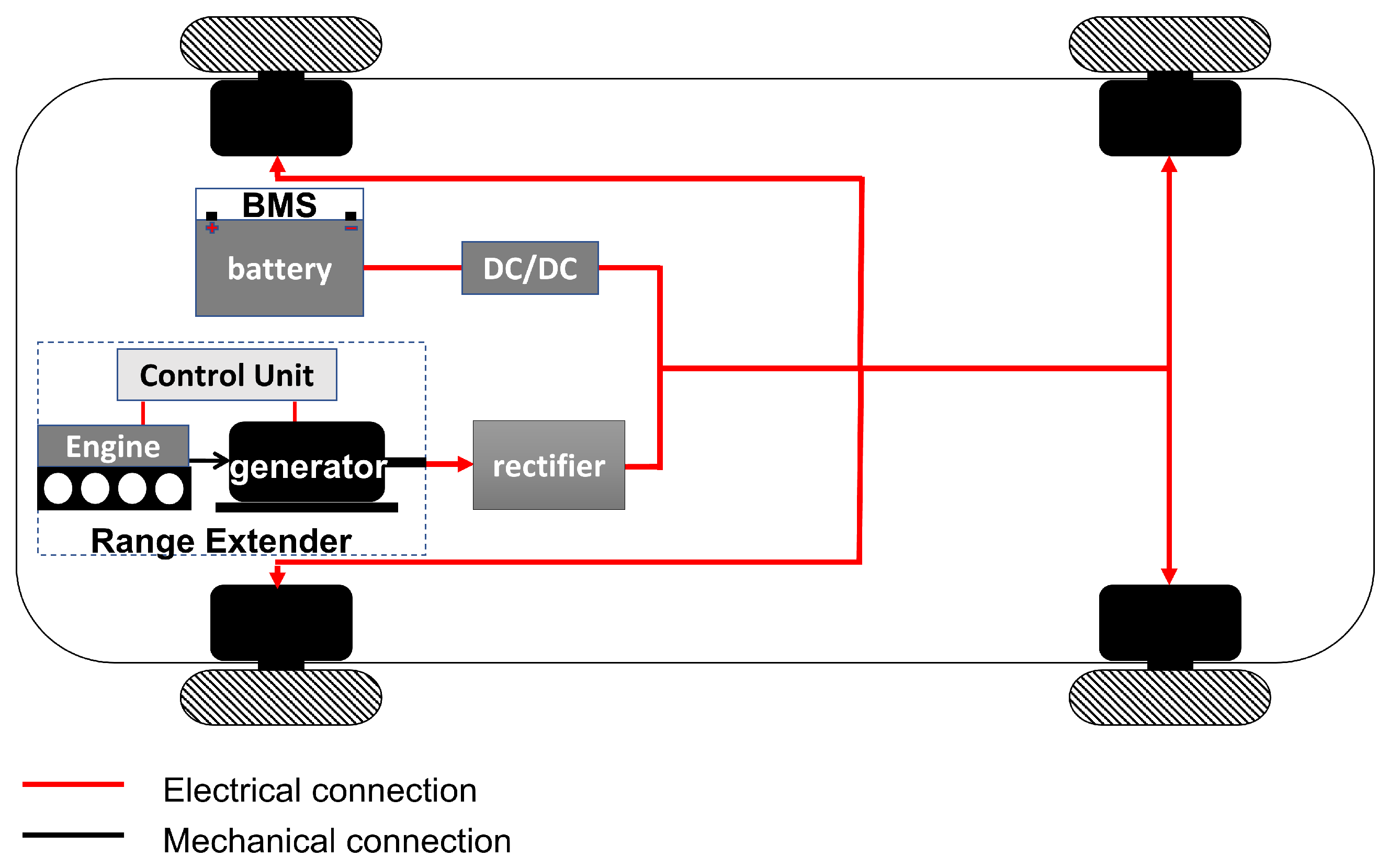
2. Powertrain Modelling
2.1. Longitudinal Dynamics Model of the Vehicle
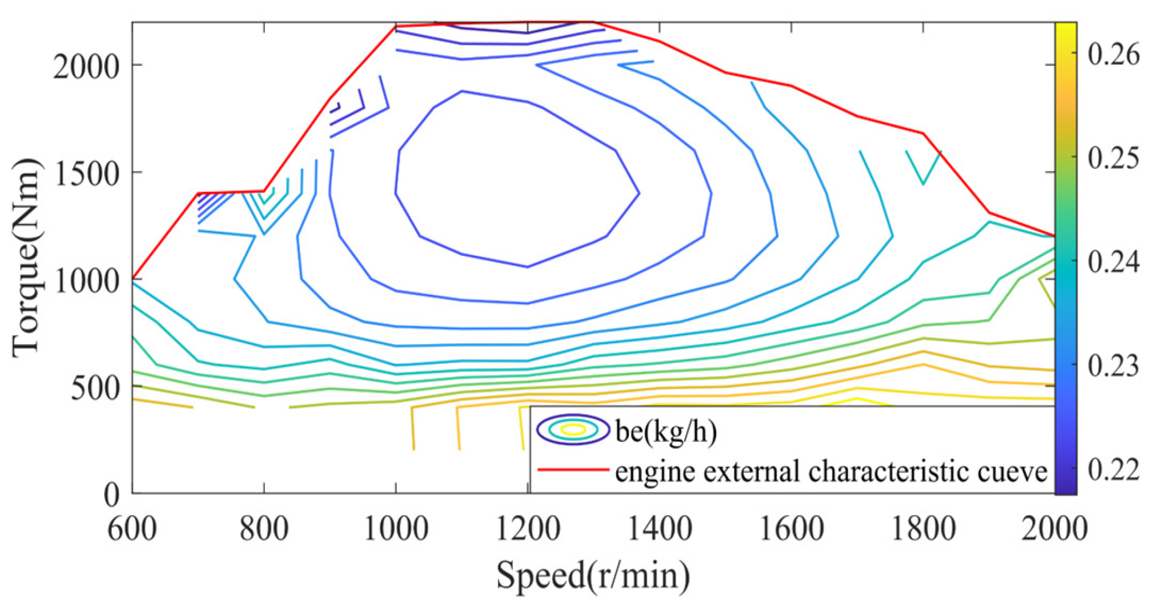
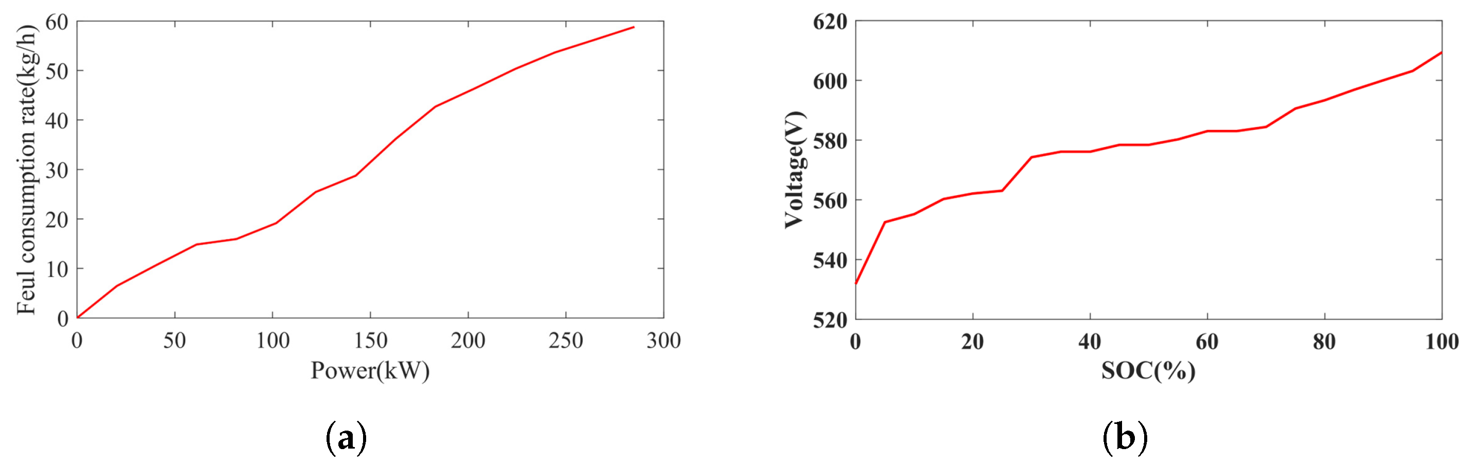
2.2. Engine Model
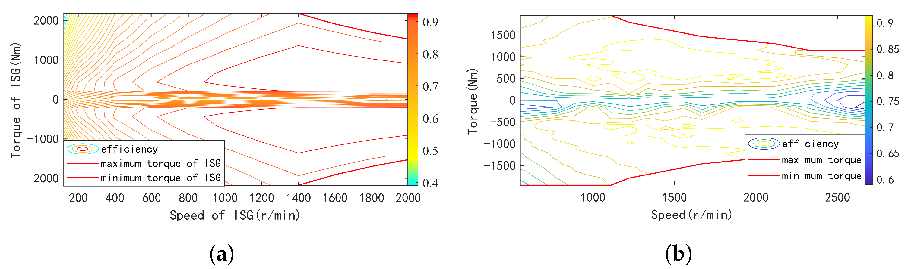
2.3. Generator and Drive Motor Models
2.4. Power Battery Model
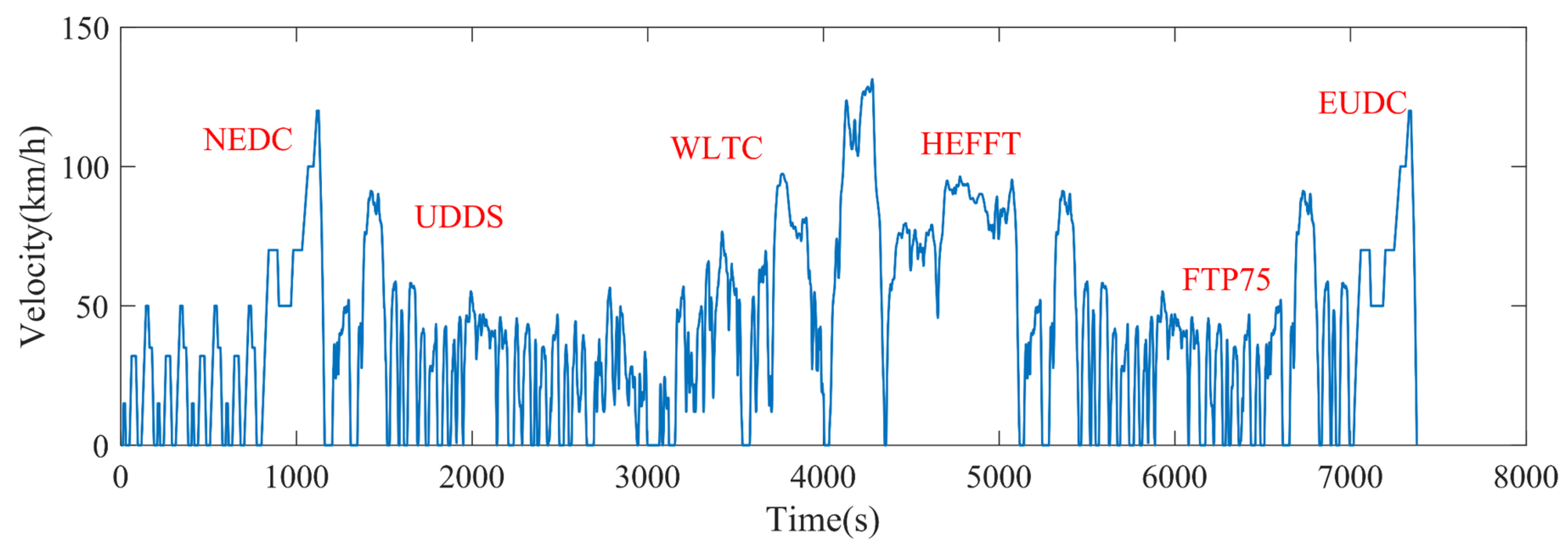
3. Speed Prediction
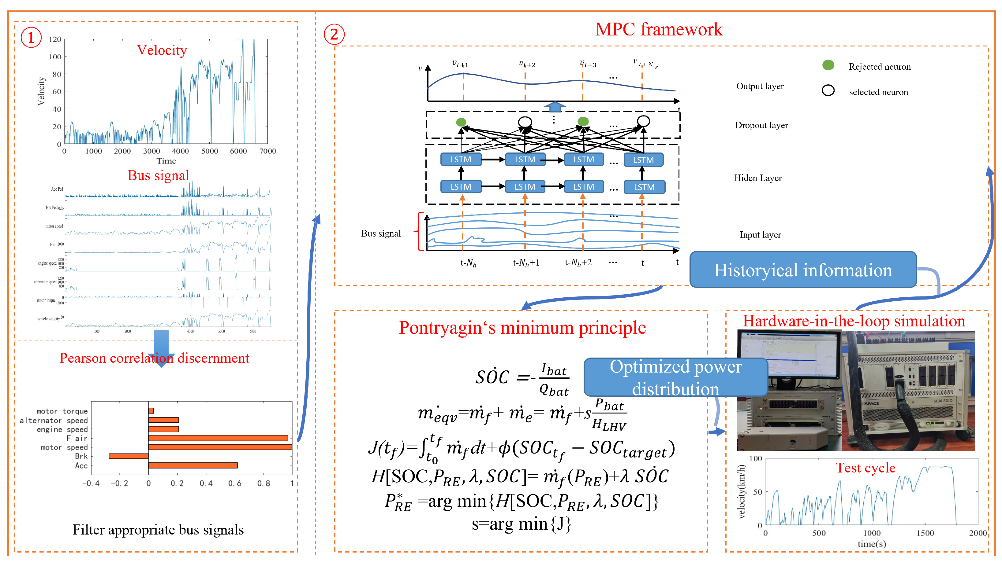
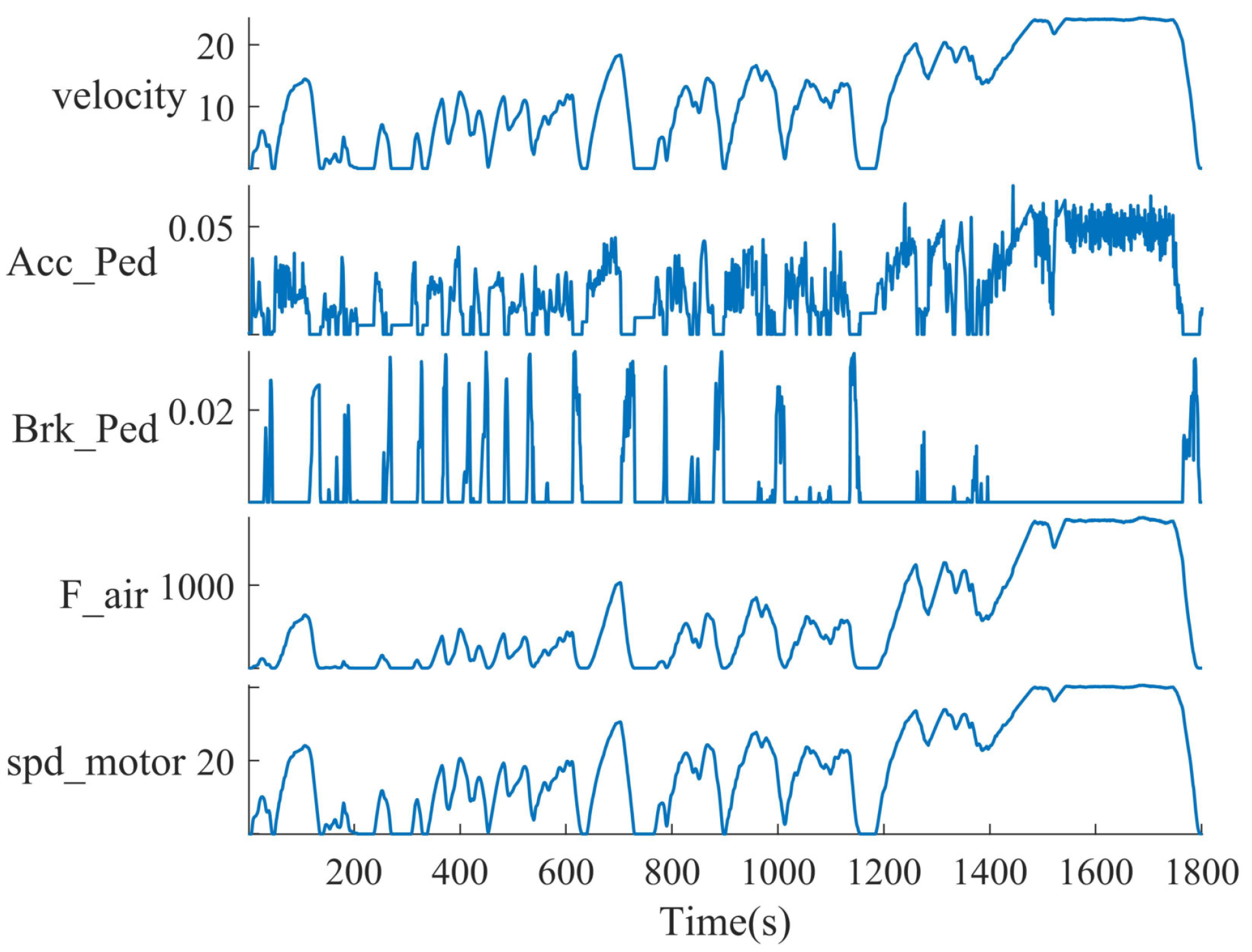
3.1. Data Processing Based on Pearson’s Correlation
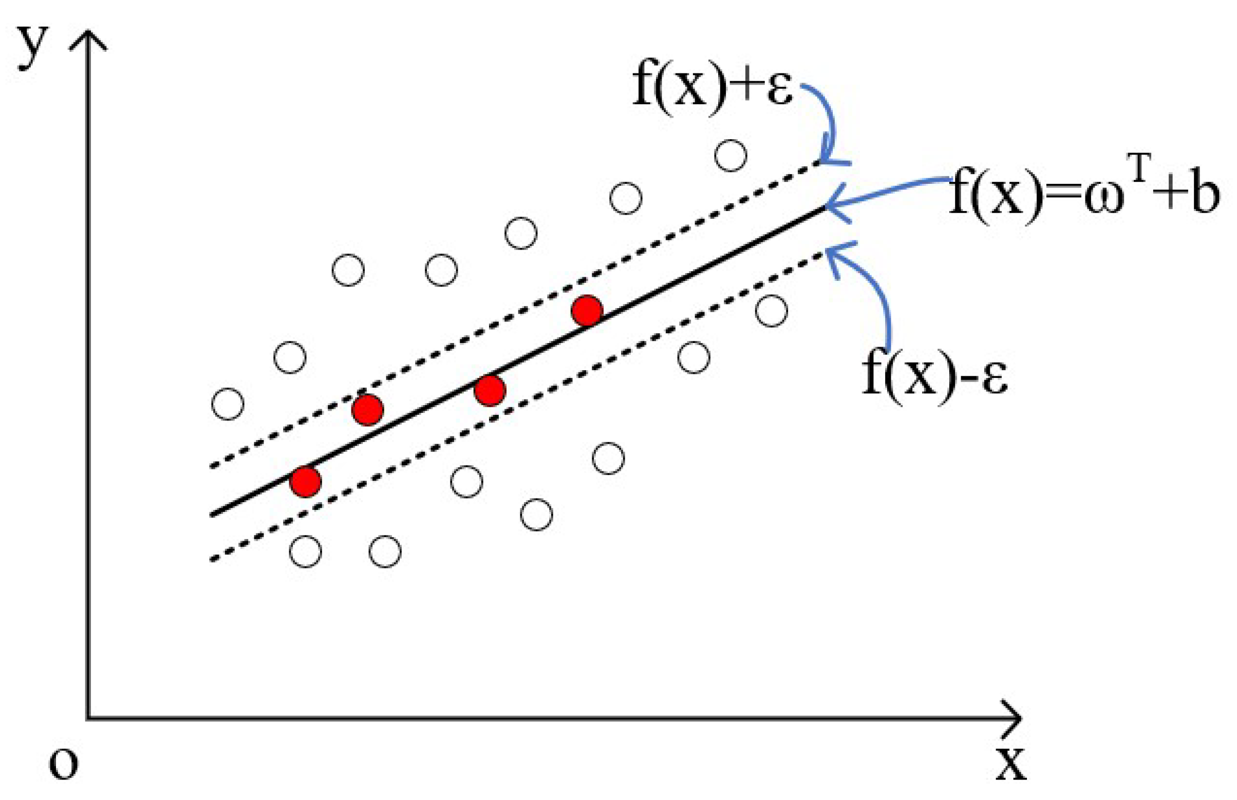
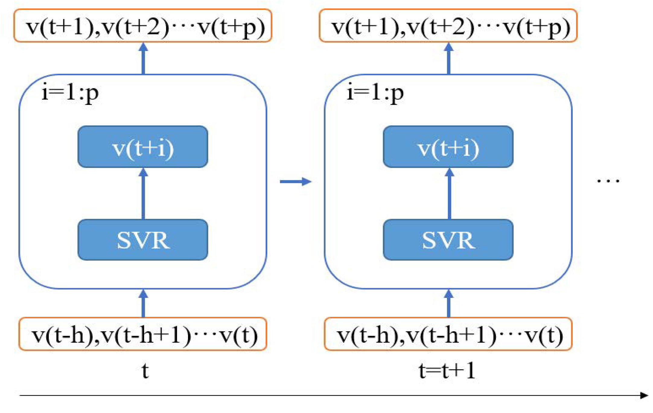
3.2. Vehicle Speed Prediction Based on SVM
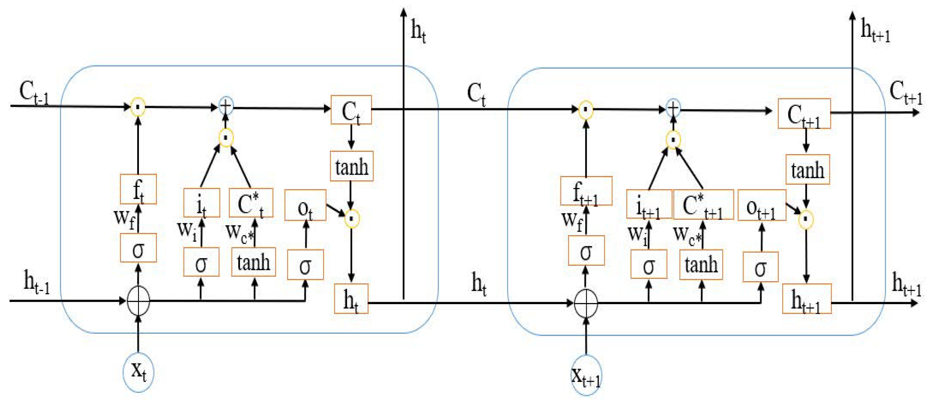
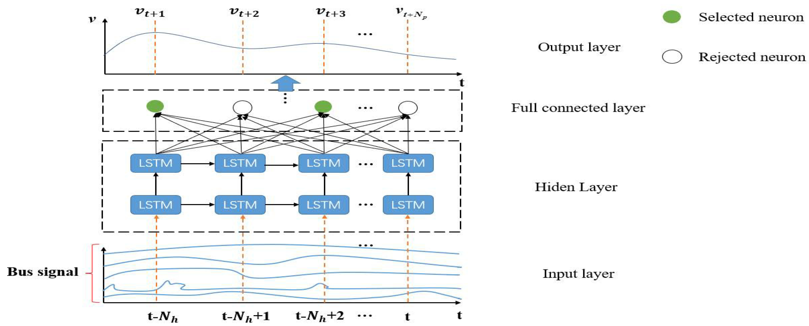
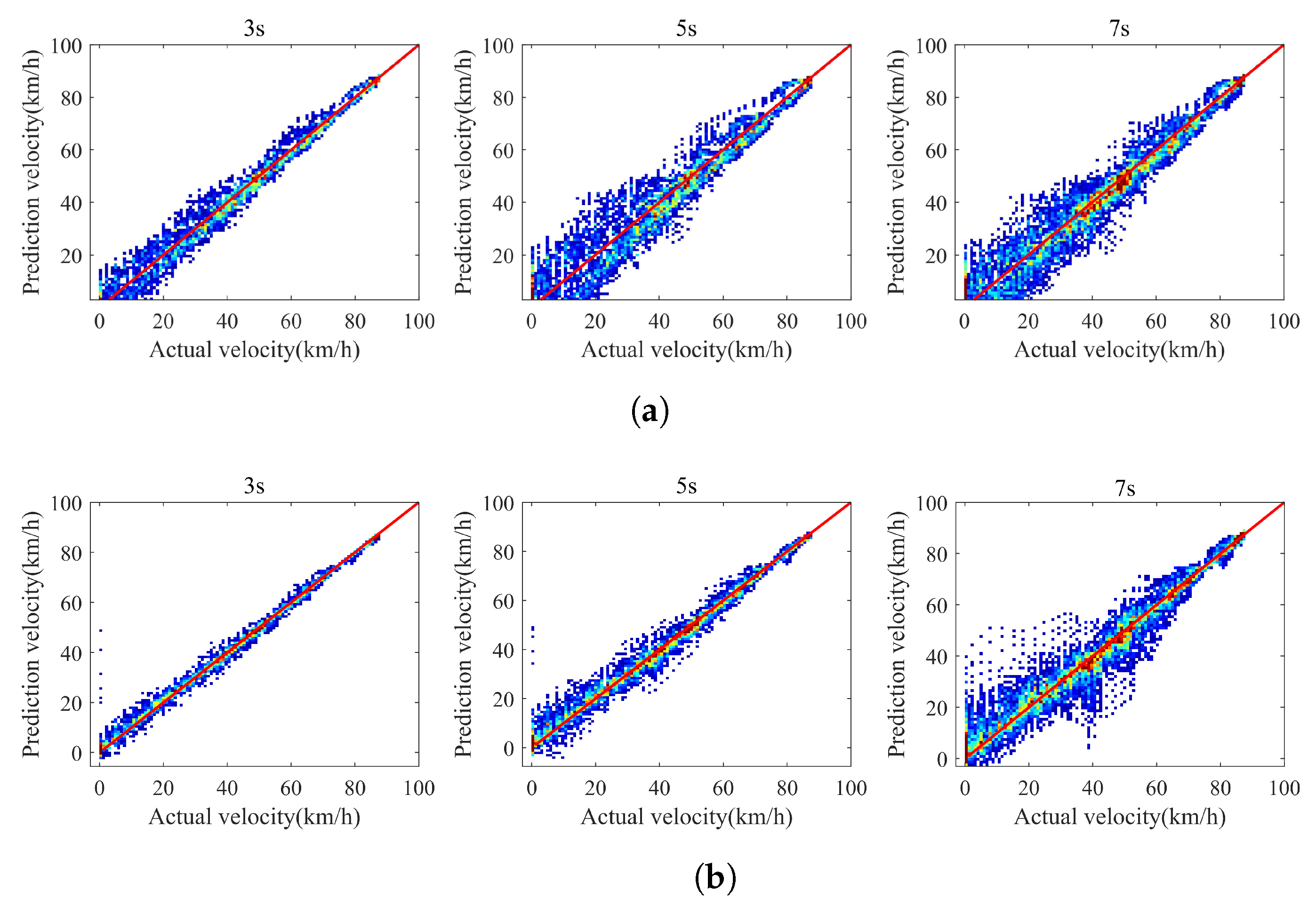
3.3. Multi-Signal Vehicle Speed Prediction Based on LSTM
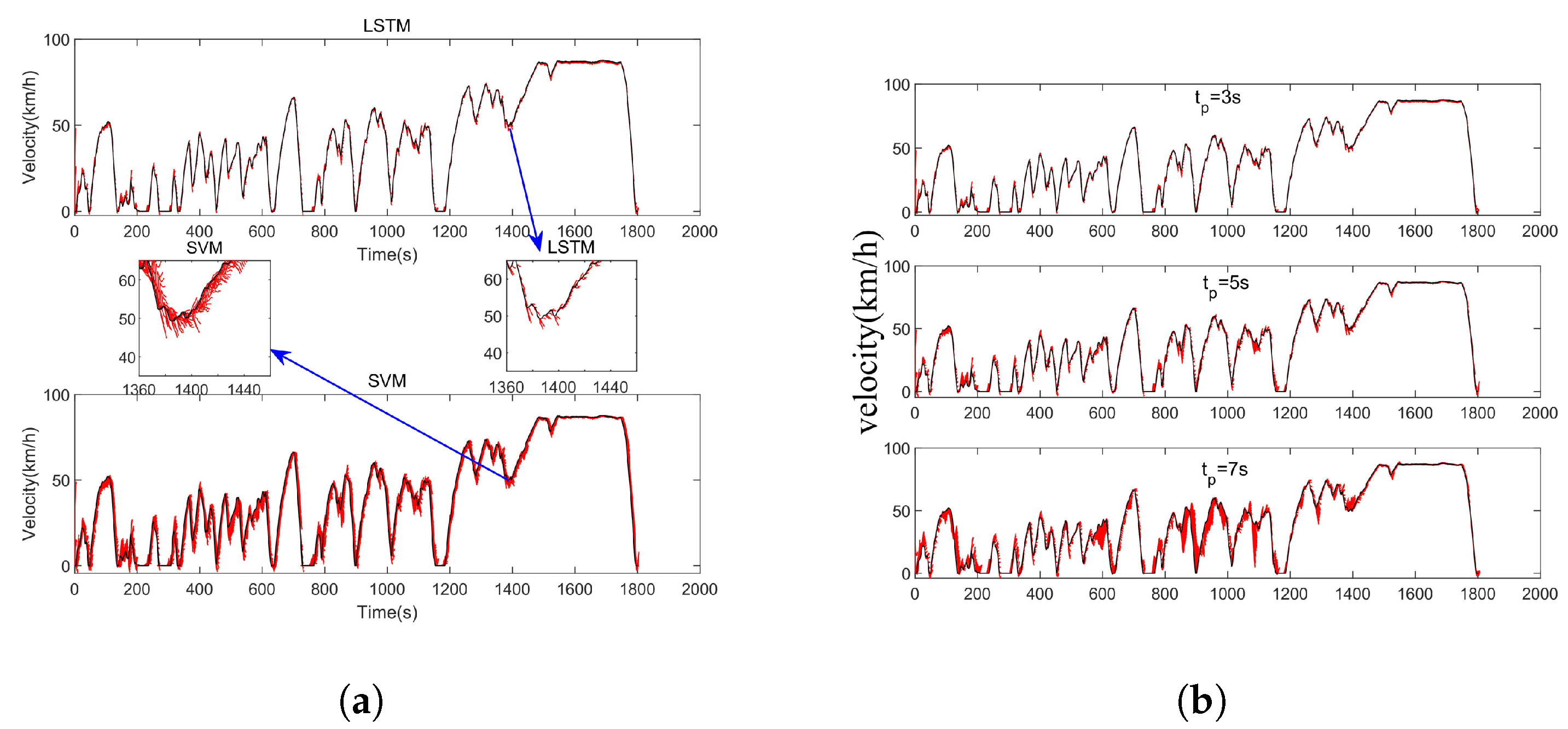
3.4. Vehicle Speed Prediction Results and Performance Comparison
4. MPC-ECMS
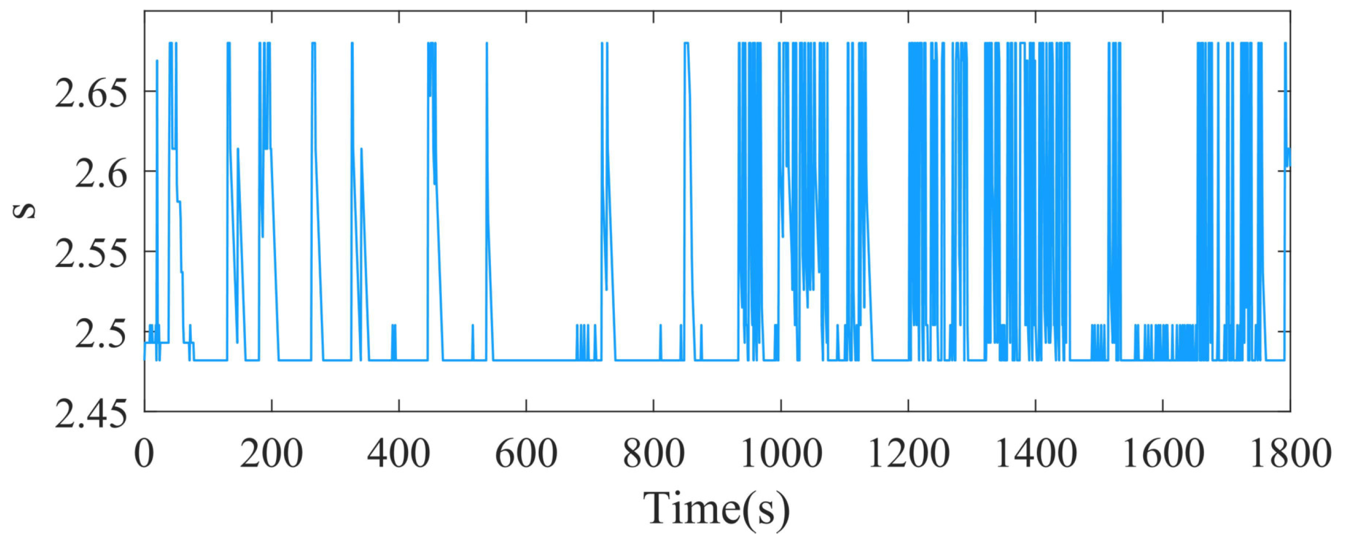
4.1. Energy Management Based on ECMS
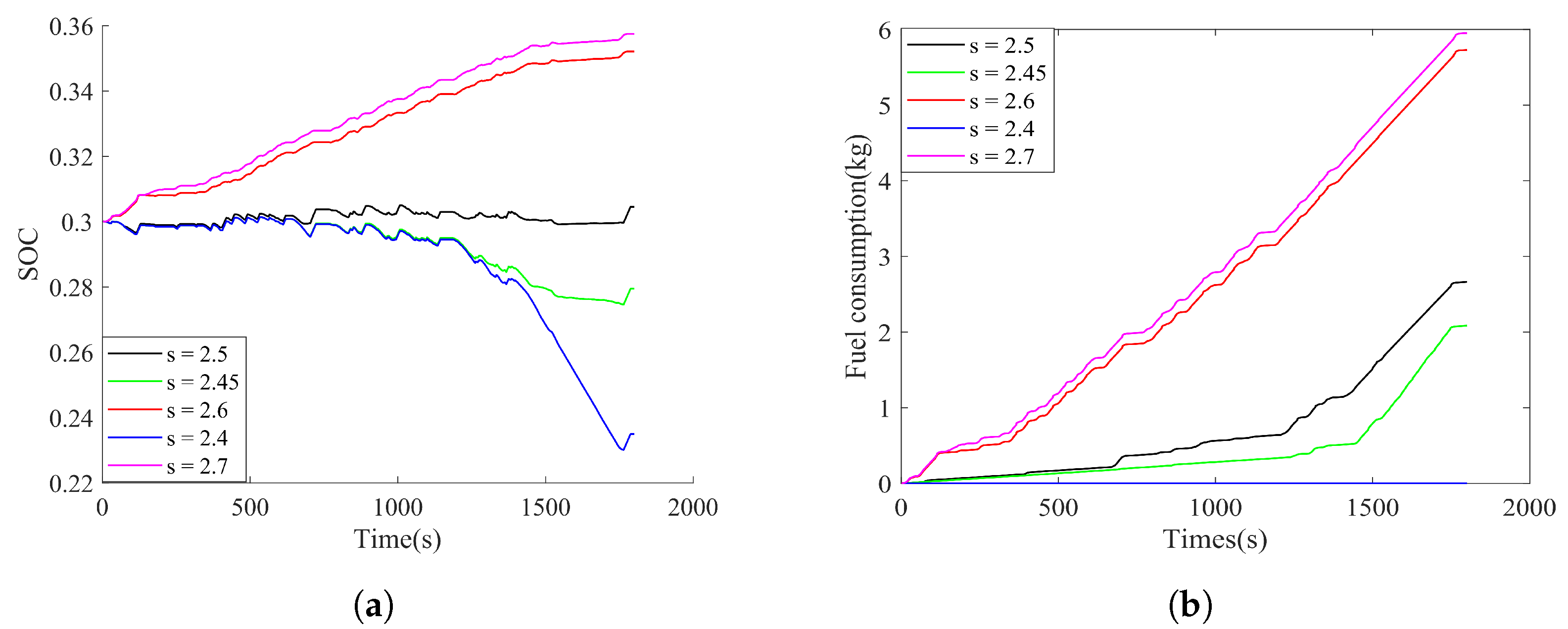
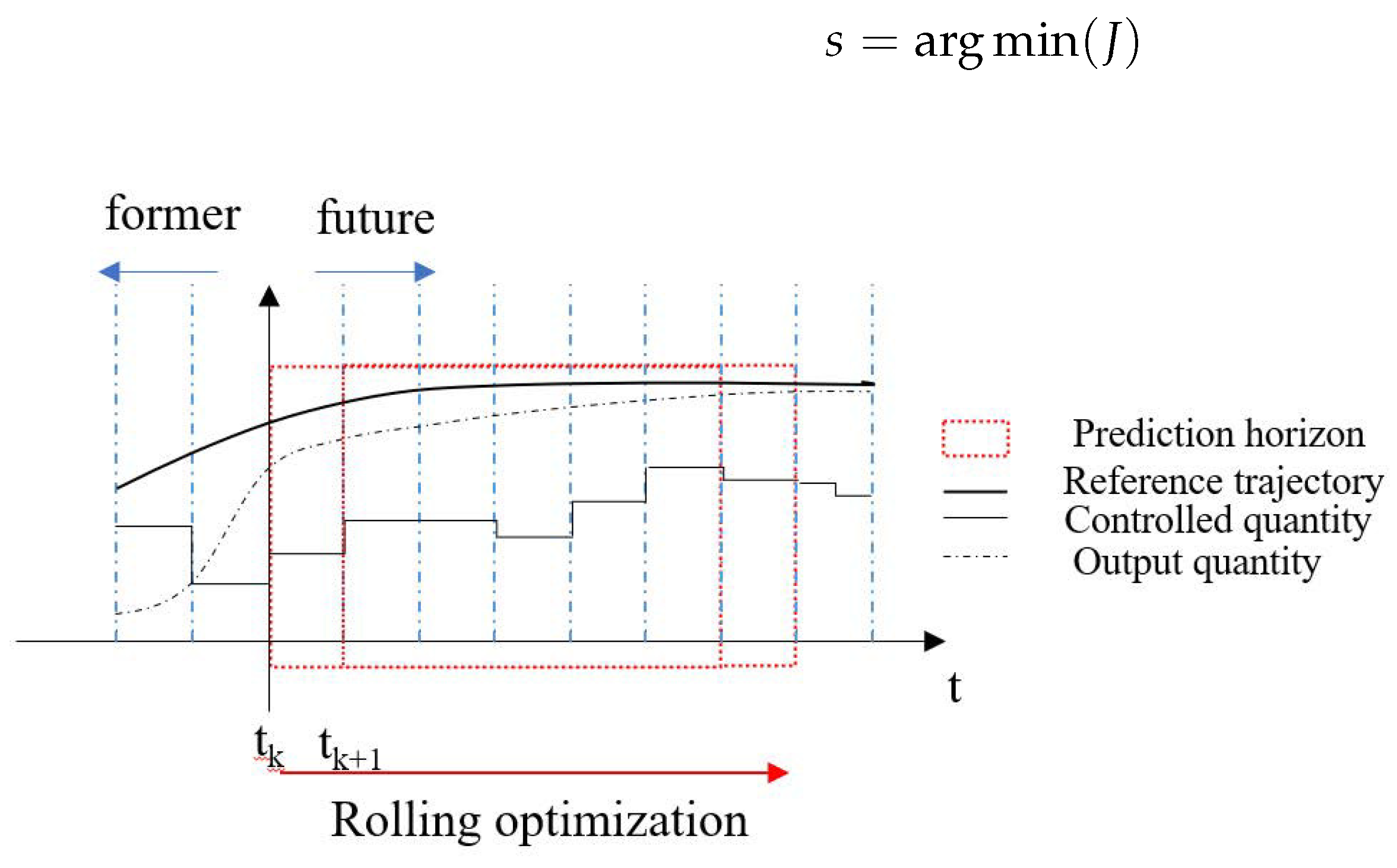
4.2. MPC-ECMS Energy Management
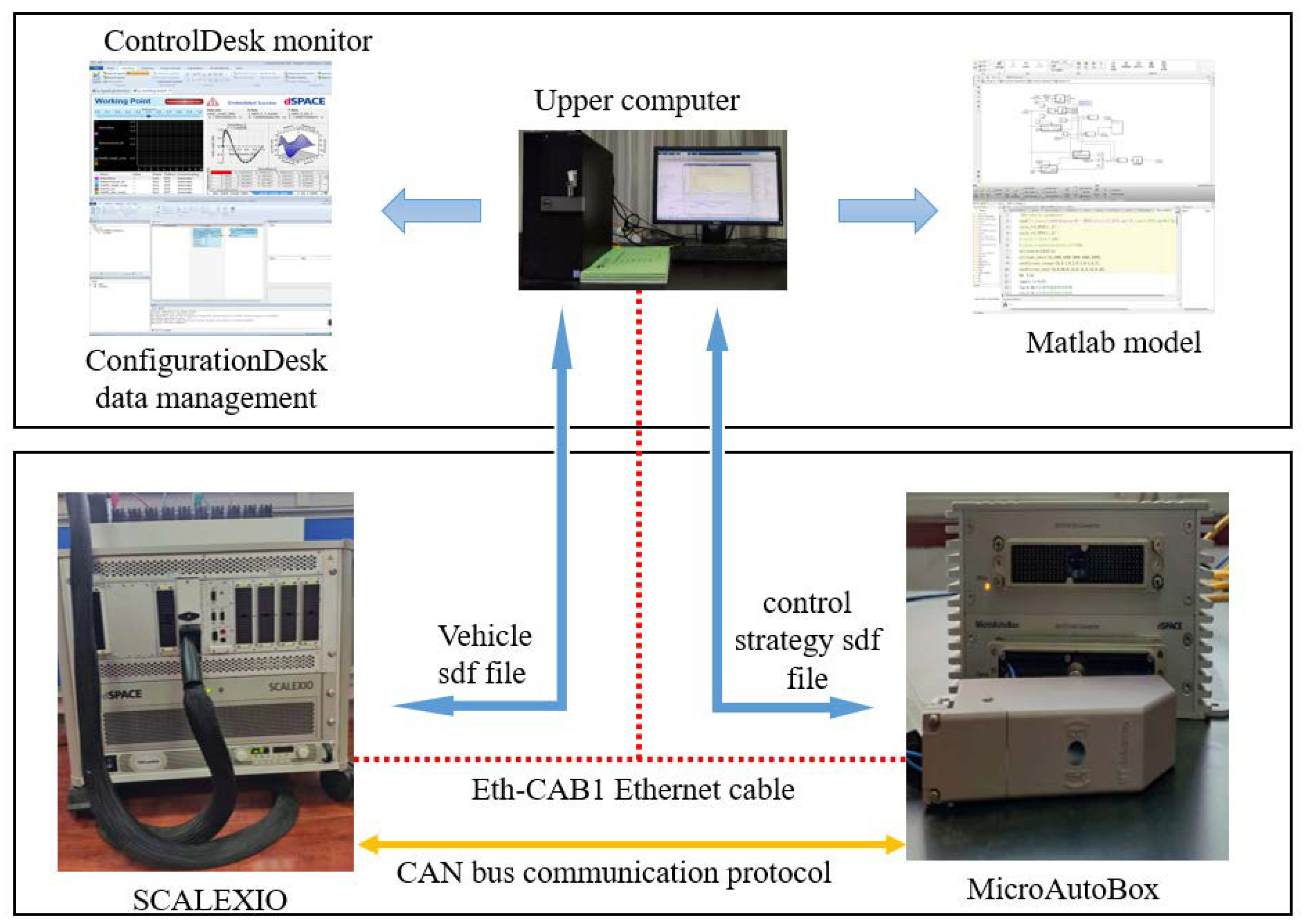
4.3. HIL Simulation Experiment
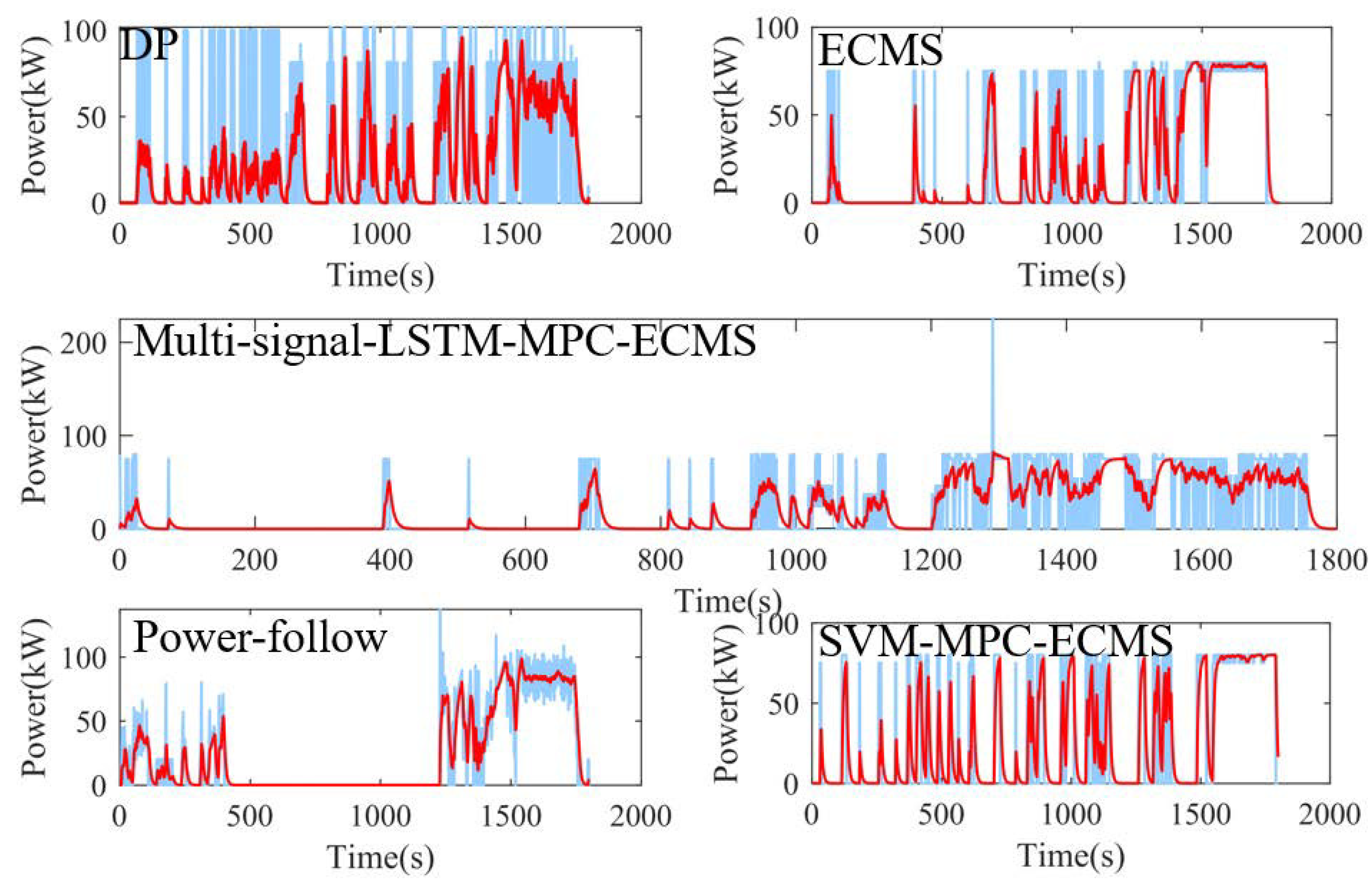
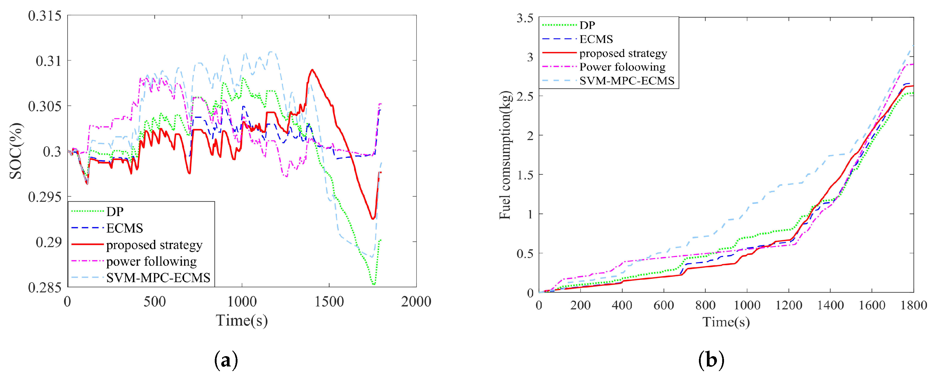
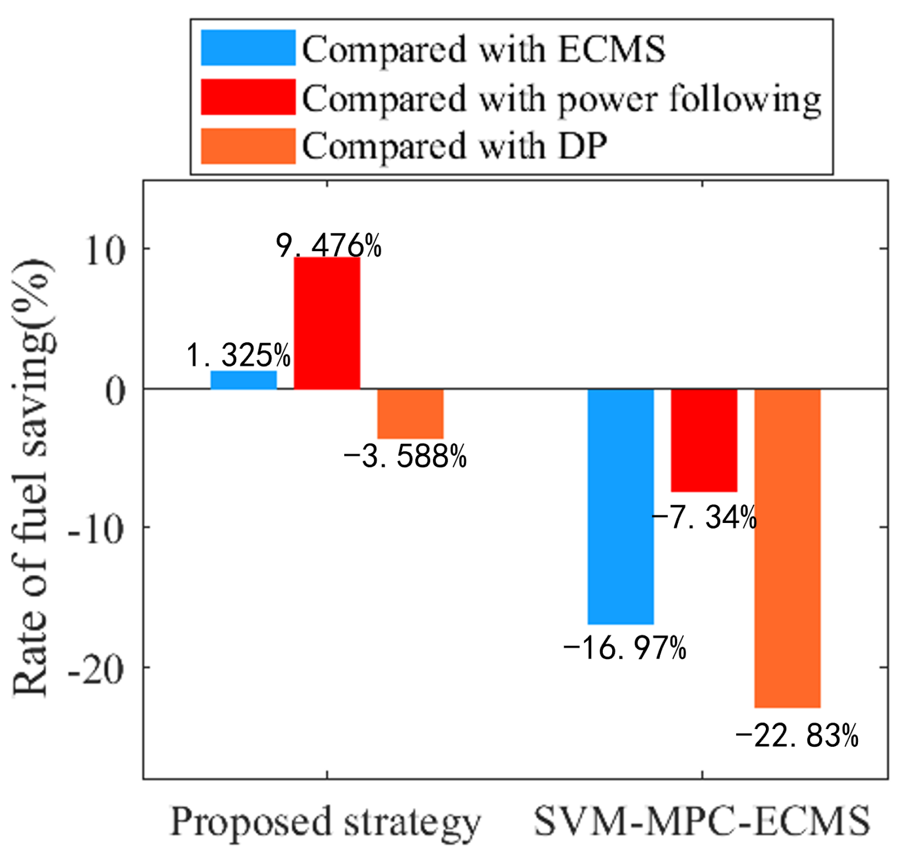
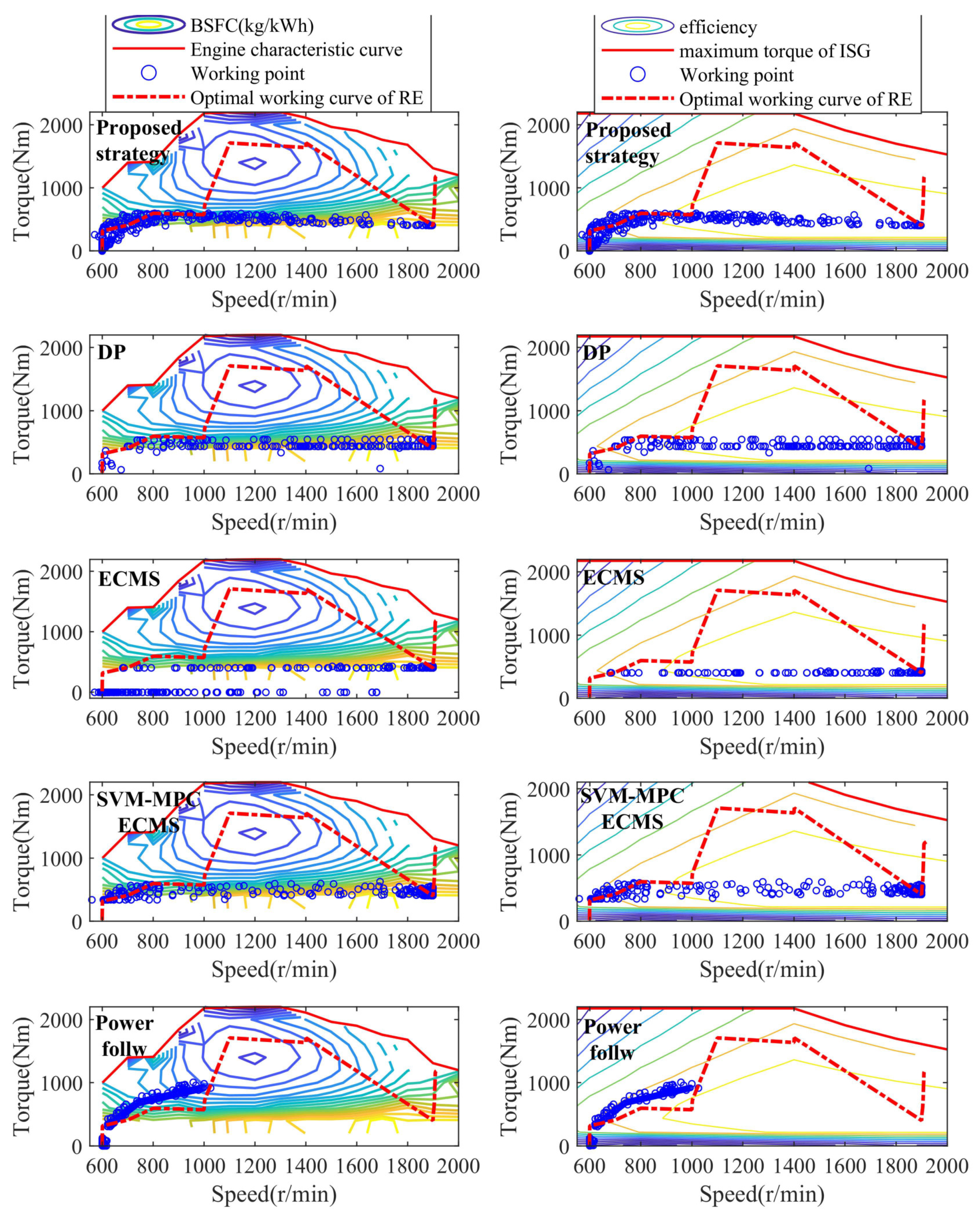
5. Results and Discussion
6. Conclusions
Author Contributions
Funding
Institutional Review Board Statement
Informed Consent Statement
Data Availability Statement
Acknowledgments
Conflicts of Interest
Abbreviations
| LSTM | Long short-term memory neural networks |
| MPC | Model predictive control |
| ECMS | Equivalent fuel consumption minimum strategy |
| SVM | Support vector machine |
| SVR | Support vector regression |
| SoC | State of charge |
| DP | Dynamic programming |
| WTVC | World transient vehicle cycle |
| HIL | Hardware-in-the-loop |
References
- Zhao, H.; Mu, L.; Li, Y.; Qiu, J.; Sun, C.; Liu, X. Unregulated Emissions from Natural Gas Taxi Based on IVE Model. Atmosphere 2021, 12, 478. [Google Scholar] [CrossRef]
- Liu, C.; Wang, Y.; Wang, L.; Chen, Z. Load-adaptive real-time energy management strategy for battery/ultracapacitor hybrid energy storage system using dynamic programming optimization. J. Power Sources 2019, 438, 227024. [Google Scholar] [CrossRef]
- Zhang, N.; Ma, X.; Jin, L. Energy management for parallel HEV based on PMP algorithm. In Proceedings of the IEEE 2017 2nd International Conference on Robotics and Automation Engineering (ICRAE), Shanghai, China, 29–31 December 2017; pp. 177–182. [Google Scholar]
- Musardo, C.; Rizzoni, G.; Guezennec, Y.; Staccia, B. A-ECMS: An adaptive algorithm for hybrid electric vehicle energy management. Eur. J. Control 2005, 11, 509–524. [Google Scholar] [CrossRef]
- Yuan, Z.; Teng, L.; Fengchun, S.; Peng, H. Comparative study of dynamic programming and Pontryagin’s minimum principle on energy management for a parallel hybrid electric vehicle. Energies 2013, 6, 2305–2318. [Google Scholar] [CrossRef]
- Zhang, H.; Fu, L.; Song, J.; Yang, Q. Power energy management and control strategy study for extended-range auxiliary power unit. Energy Procedia 2016, 104, 32–37. [Google Scholar] [CrossRef]
- Chen, B.C.; Wu, Y.Y.; Tsai, H.C. Design and analysis of power management strategy for range extended electric vehicle using dynamic programming. Appl. Energy 2014, 113, 1764–1774. [Google Scholar] [CrossRef]
- Pan, C.; Liang, Y.; Chen, L.; Chen, L. Optimal control for hybrid energy storage electric vehicle to achieve energy saving using dynamic programming approach. Energies 2019, 12, 588. [Google Scholar] [CrossRef] [Green Version]
- Rezaei, A.; Burl, J.B.; Zhou, B. Estimation of the ECMS equivalent factor bounds for hybrid electric vehicles. IEEE Trans. Control. Syst. Technol. 2017, 26, 2198–2205. [Google Scholar] [CrossRef]
- Yu, X.; Lin, C.; Tian, Y.; Zhao, M.; Liu, H.; Xie, P.; Zhang, J. Real-time and hierarchical energy management-control framework for electric vehicles with dual-motor powertrain system. Energy 2023, 272, 127112. [Google Scholar] [CrossRef]
- Shen, P.; Zhao, Z.; Zhan, X.; Li, J.; Guo, Q. Optimal energy management strategy for a plug-in hybrid electric commercial vehicle based on velocity prediction. Energy 2018, 155, 838–852. [Google Scholar] [CrossRef]
- Wang, W.; Guo, X.; Yang, C.; Zhang, Y.; Zhao, Y.; Huang, D.; Xiang, C. A multi-objective optimization energy management strategy for power split HEV based on velocity prediction. Energy 2022, 238, 121714. [Google Scholar] [CrossRef]
- Xing, J.; Chu, L.; Hou, Z.; Sun, W.; Zhang, Y. Energy Management Strategy Based on a Novel Speed Prediction Method. Sensors 2021, 21, 8273. [Google Scholar] [CrossRef]
- Chen, R.; Yang, C.; Han, L.; Wang, W.; Ma, Y.; Xiang, C. Power reserve predictive control strategy for hybrid electric vehicle using recognition-based long short-term memory network. J. Power Sources 2022, 520, 230865. [Google Scholar] [CrossRef]
- Han, J.; Shu, H.; Tang, X.; Lin, X.; Liu, C.; Hu, X. Predictive energy management for plug-in hybrid electric vehicles considering electric motor thermal dynamics. Energy Convers. Manag. 2022, 251, 115022. [Google Scholar] [CrossRef]
- Lin, X.; Wu, J.; Wei, Y. An ensemble learning velocity prediction-based energy management strategy for a plug-in hybrid electric vehicle considering driving pattern adaptive reference SOC. Energy 2021, 234, 121308. [Google Scholar] [CrossRef]
- Ritter, A.; Widmer, F.; Duhr, P.; Onder, C.H. Long-term stochastic model predictive control for the energy management of hybrid electric vehicles using Pontryagin’s minimum principle and scenario-based optimization. Appl. Energy 2022, 322, 119192. [Google Scholar] [CrossRef]
- Li, M.; He, H.; Feng, L.; Chen, Y.; Yan, M. Hierarchical predictive energy management of hybrid electric buses based on driver information. J. Clean. Prod. 2020, 269, 122374. [Google Scholar] [CrossRef]
- Wei, C.; Chen, Y.; Li, X.; Lin, X. Integrating intelligent driving pattern recognition with adaptive energy management strategy for extender range electric logistics vehicle. Energy 2022, 247, 123478. [Google Scholar] [CrossRef]
- Chen, Z.; Gu, H.; Shen, S.; Shen, J. Energy management strategy for power-split plug-in hybrid electric vehicle based on MPC and double Q-learning. Energy 2022, 245, 123182. [Google Scholar] [CrossRef]
- Lin, X.; Zhang, J.; Su, L. A trip distance adaptive real-time optimal energy management strategy for a plug-in hybrid vehicle integrated driving condition prediction. J. Energy Storage 2022, 52, 105055. [Google Scholar] [CrossRef]
- Zhao, Z.; Xun, J.; Wan, X.; Yu, R. Mpc based hybrid electric vehicles energy management strategy. IFAC-PapersOnLine 2021, 54, 370–375. [Google Scholar] [CrossRef]
- Wang, Y.; Zhang, Y.; Zhang, C.; Zhou, J.; Hu, D.; Yi, F.; Fan, Z.; Zeng, T. Genetic algorithm-based fuzzy optimization of energy management strategy for fuel cell vehicles considering driving cycles recognition. Energy 2023, 263, 126112. [Google Scholar] [CrossRef]
- Zhou, Y.; Ravey, A.; Péra, M.C. Multi-mode predictive energy management for fuel cell hybrid electric vehicles using Markov driving pattern recognizer. Appl. Energy 2020, 258, 114057. [Google Scholar] [CrossRef]
- Türker, E.; Bulut, E.; Kahraman, A.; Çakıcı, M.; Öztürk, F. Estimation of Energy Management Strategy Using Neural-Network-Based Surrogate Model for Range Extended Vehicle. Appl. Sci. 2022, 12, 12935. [Google Scholar] [CrossRef]
- Al-Saadi, Z.; Phan Van, D.; Moradi Amani, A.; Fayyazi, M.; Sadat Sajjadi, S.; Ba Pham, D.; Jazar, R.; Khayyam, H. Intelligent Driver Assistance and Energy Management Systems of Hybrid Electric Autonomous Vehicles. Sustainability 2022, 14, 9378. [Google Scholar] [CrossRef]
- Wang, H.; Huang, Y.; Khajepour, A.; Song, Q. Model predictive control-based energy management strategy for a series hybrid electric tracked vehicle. Appl. Energy 2016, 182, 105–114. [Google Scholar] [CrossRef] [Green Version]
- Mu, L.; Zhao, H.; Li, Y.; Liu, X.; Qiu, J.; Sun, C. Traffic flow statistics method based on deep learning and multi-feature fusion. CMES Comput. Model. Eng. Sci. 2021, 129, 465–483. [Google Scholar] [CrossRef]
- Hong, J.; Wang, Z.; Qu, C.; Zhou, Y.; Shan, T.; Zhang, J.; Hou, Y. Investigation on overcharge-caused thermal runaway of lithium-ion batteries in real-world electric vehicles. Appl. Energy 2022, 321, 119229. [Google Scholar] [CrossRef]
- Hong, J.; Zhang, H.; Xu, X. Thermal fault prognosis of lithium-ion batteries in real-world electric vehicles using self-attention mechanism networks. Appl. Therm. Eng. 2023, 226, 120304. [Google Scholar] [CrossRef]
- Sun, X.; Fu, J.; Yang, H.; Xie, M.; Liu, J. An energy management strategy for plug-in hybrid electric vehicles based on deep learning and improved model predictive control. Energy 2023, 269, 126772. [Google Scholar] [CrossRef]


| Name | Parameters | Value | Parameters | Value |
|---|---|---|---|---|
| Vehicle | Total mass | 7000 kg | Wheel radius | 0.60 m |
| Aerodynamic drag coefficient | 0.6 | Front area | 9 m | |
| Engine | Engine type | Diesel engine | Maximum torque | 2200 Nm |
| Maximum speed | 2000 r/min | |||
| Electric motor | Maximum torque | 1800 Nm | Maximum speed | 2650 r/min |
| Type | Permanent magnet synchronous | |||
| Generator | Maximum torque | 2200 Nm | Maximum speed | 2000 r/min |
| Battery pack | Voltage | 580 V | Capacity | 200 Ah |
| CAN Bus Signal | Pearson’s Correlation Coefficient |
|---|---|
| Accelerator pedal opening | 0.6192 |
| Brake pedal opening | −0.2737 |
| Motor speed | 1 |
| Air resistance | 0.9687 |
| Engine speed | 0.2085 |
| Alternator speed | 0.2085 |
| Motor torque | 0.0356 |
| Multi-Signal LSTM | SVM | |||
|---|---|---|---|---|
| (s) | RMSE | (s) | RMSE | |
| 3 s | 0.0044 | 1.6085 | 0.00611 | 2.3735 |
| 5 s | 0.0034 | 3.0936 | 0.009597 | 4.2482 |
| 7 s | 0.0045 | 6.6171 | 0.0234 | 6.9404 |
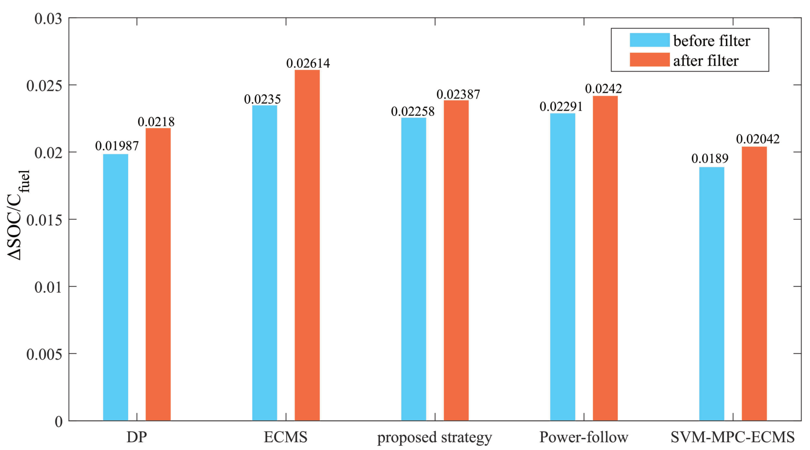
| Control Strategy | SoC | Fuel Consumption (kg) | ||
|---|---|---|---|---|
| Pre-Filter | After-Filter | Pre-Filter | After-Filter | |
| DP | 0.2938 | 0.2902 | 2.9637 | 2.536 |
| ECMS ( 2.5) | 0.308 | 0.3045 | 3.112 | 2.663 |
| Multi-signal-LSTM-MPC-ECMS | 0.3031 | 0.2976 | 3.02 | 2.627 |
| Power-follow | 0.306 | 0.3052 | 3.103 | 2.902 |
| SVM-MPC-ECMS | 0.3013 | 0.2985 | 3.505 | 3.115 |
Disclaimer/Publisher’s Note: The statements, opinions and data contained in all publications are solely those of the individual author(s) and contributor(s) and not of MDPI and/or the editor(s). MDPI and/or the editor(s) disclaim responsibility for any injury to people or property resulting from any ideas, methods, instructions or products referred to in the content. |
© 2023 by the authors. Licensee MDPI, Basel, Switzerland. This article is an open access article distributed under the terms and conditions of the Creative Commons Attribution (CC BY) license (https://creativecommons.org/licenses/by/4.0/).
Share and Cite
Lu, L.; Zhao, H.; Liu, X.; Sun, C.; Zhang, X.; Yang, H. MPC-ECMS Energy Management of Extended-Range Vehicles Based on LSTM Multi-Signal Speed Prediction. Electronics 2023, 12, 2642. https://doi.org/10.3390/electronics12122642
Lu L, Zhao H, Liu X, Sun C, Zhang X, Yang H. MPC-ECMS Energy Management of Extended-Range Vehicles Based on LSTM Multi-Signal Speed Prediction. Electronics. 2023; 12(12):2642. https://doi.org/10.3390/electronics12122642
Chicago/Turabian StyleLu, Laiwei, Hong Zhao, Xiaotong Liu, Chuanlong Sun, Xinyang Zhang, and Haixu Yang. 2023. "MPC-ECMS Energy Management of Extended-Range Vehicles Based on LSTM Multi-Signal Speed Prediction" Electronics 12, no. 12: 2642. https://doi.org/10.3390/electronics12122642