Monocular Depth Estimation for 3D Map Construction at Underground Parking Structures

Abstract

Converting the actual scenes into three-dimensional models has inevitably become one of the fundamental requirements in autonomous driving. At present, the main obstacle to large-scale deployment is the high-cost lidar for environment sensing. Monocular depth estimation aims to predict the scene depth and construct a 3D map via merely a monocular camera. In this paper, we add geometric consistency constraints to address the non-Lambertian surface problems in depth estimation. We also utilize the imaging principles and conversion rules to produce a 3D scene model from multiple images. We built a prototype and conduct extensive experiments in a corridor and an underground parking structure, and the results show the effectiveness for indoor location-based services.

1. Introduction

Autonomous vehicles [1] are required to identify roads and obstacles [2] for fine-grained path planning. Among all crucial autopilot techniques, it is quite important to predict monocular depth in front of the vehicle; thus, it becomes a hot research topic in both academy and industry.

The mature solution for depth estimation is based on radar ranging [3,4], which requires a radar ranging device at a designated location on the vehicle to sense the road information. However, radar ranging has certain drawbacks, including high equipment costs [5], inconvenient installation [6], and unfavorable deployment. Therefore, this paper adopts another cost-effective solution, i.e., using a monocular image for depth estimation. Currently, there are still several limitations in monocular depth estimation, including large errors, difficulties in data acquisition, and complex model training.

Thanks to the rapid development of deep learning, the existing monocular depth estimation techniques now consist of supervised learning and unsupervised learning [7,8,9]. Among them, although the supervised monocular depth prediction obtains higher accuracy, the training cost is extremely large due to the difficulty in acquiring the ground truth depth. In this paper, we propose an unsupervised learning method for monocular depth estimation.

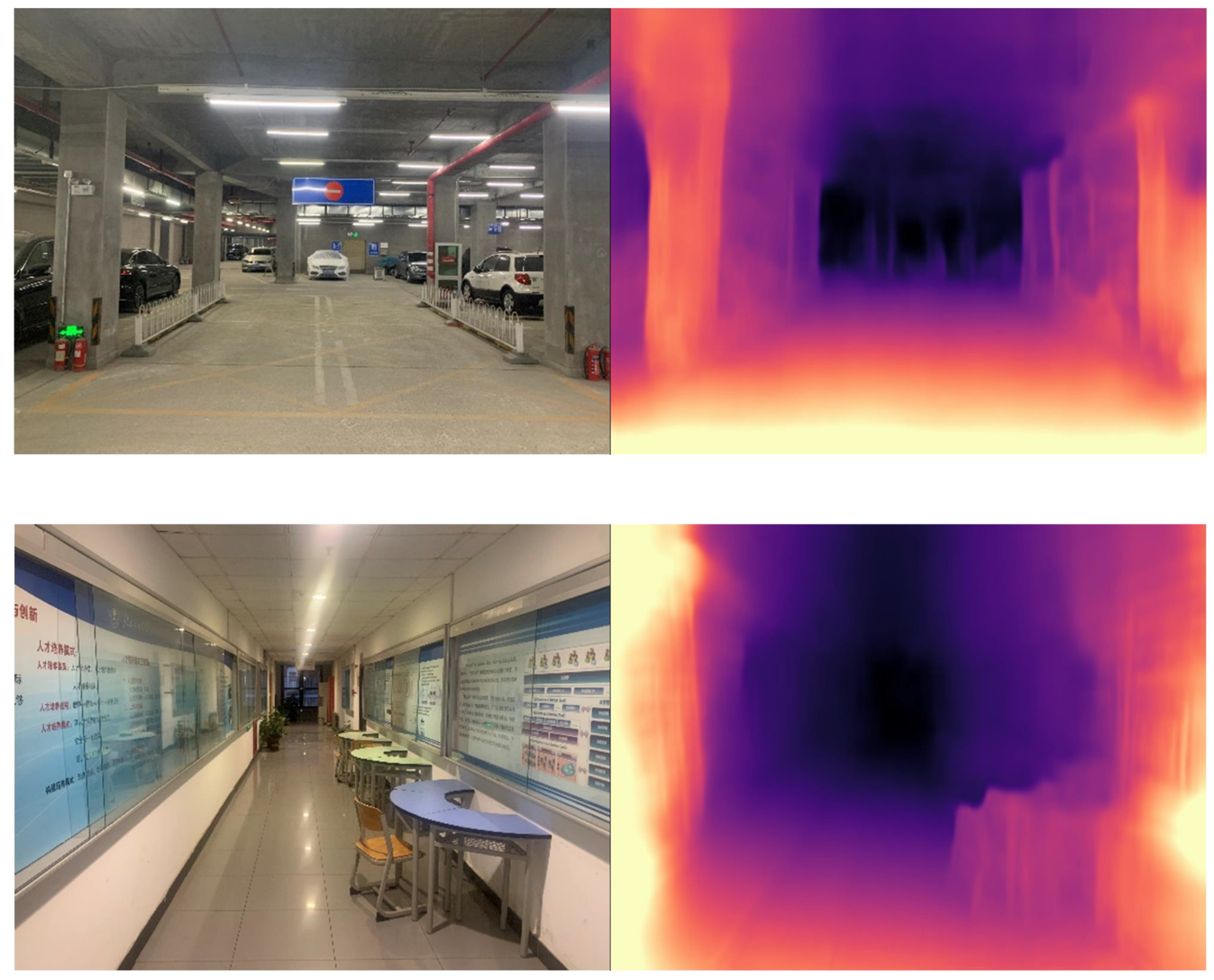
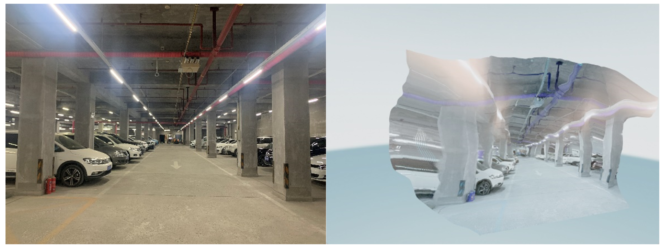
The main problem solved in this paper is to use monocular vision to extract unsupervised depth estimation model and depth map from continuous video clips, construct point clouds to obtain complete 3D modeling and configure the system to an intelligent remote control car. Although monocular depth estimation has been widely adopted in autonomous driving, it largely relies on texture features with proper illumination; thus, it is not suitable in GPS blocked environments such as tunnels and underground parking structures.

In this paper, we leverage the geometric consistency to improve the depth prediction accuracy, and propose a lightweight 3D scene construction method via only single image. Specially, based on camera imaging principles, we reconstruct the 3D scene of the depth map, and color the 3D model by the colorful pixels from the RGB image. This colored three-dimensional color image makes the depth estimation results more intuitive and facilitate further analysis.

Our contributions include:

• We propose a unsupervised deep learning method for monocular depth estimation, and design a geometric consistency loss to enhance the robustness in extreme environments (Section 3). The method avoids the tedious steps of manual calibration and reduces the cost of manpower and material for ground truth labelling.
• We devise a three-dimensional modeling approach which converts a planar image stream into a three-dimensional point cloud model, with low restrictions on the scene and few requirements for shooting (Section 4).
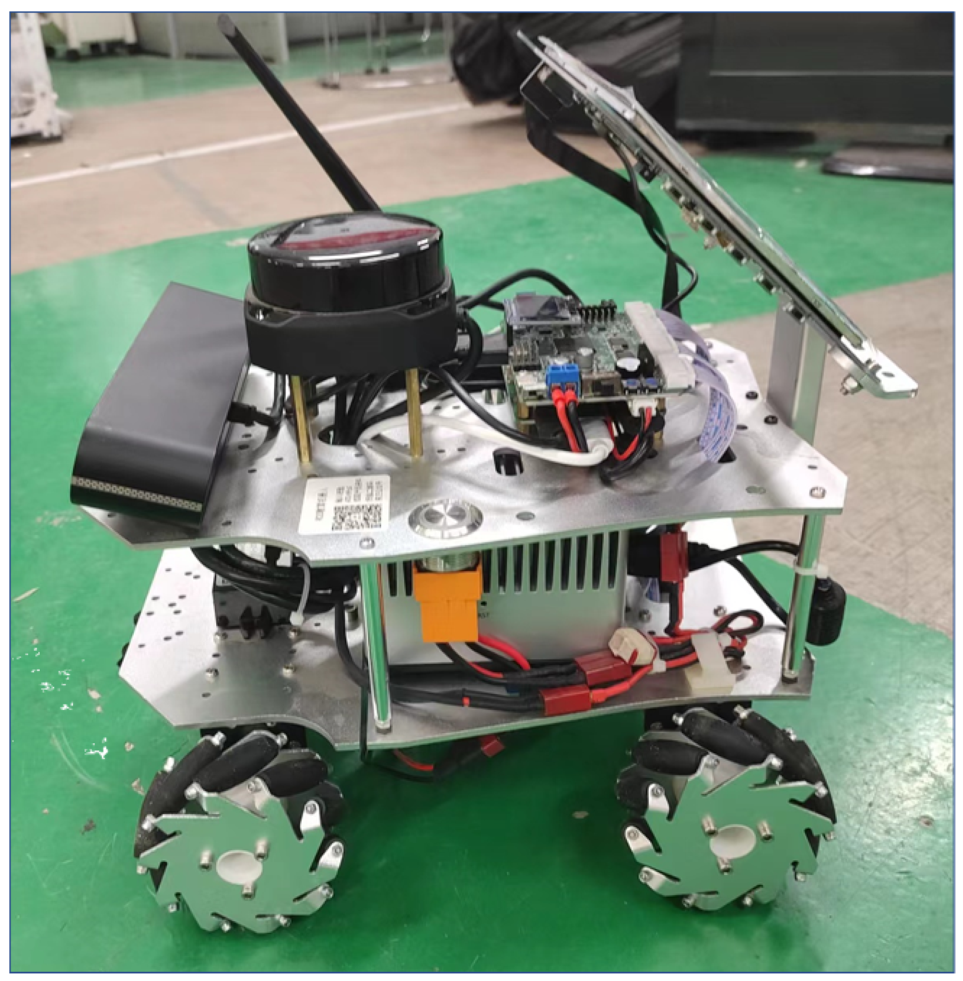
• We developed a prototype system for our autonomous vehicles, and conducted extensive experiments in real-world scenarios. The results show the effectiveness of our system (Section 5).

The remainder of this article is organized as follows. In the second section, we introduce the background and technical foundation of our work, and discuss the two parts of “monocular” and “unsupervised”, respectively. In the third section, we introduce the monocular depth estimation algorithm used in our experiment, focusing on the principles and methods of introducing depth rendering and geometric consistency loss to the system. In the fourth section, we introduced the principles and methods of point cloud model transformation used in the experiment. In the fifth section, we configure the system on the ROS smart car to carry out the experiment. In this section, we present and quantify the results of depth map transformation and point cloud model generation. We summarize the experiments in the sixth section.

2. Related Work

In this paper, the strategy of unsupervised monocular depth estimation is adopted for depth recognition, and the transformed point cloud array is used for three-dimensional modeling. Among them, the implementation methods of depth estimation can be mainly divided into radar ranging and RGB image conversion. The RGB depth estimation algorithm is combined with monocular and binocular depth estimation, and combined with deep learning when building the depth conversion model.

2.1. RGB Depth Estimation Algorithm

Using RGB solutions, binocular image depth estimation is a more classical and mature depth estimation algorithm based on the stereo matching technology that emerged in the 1980s. In 2016, Nikolaus and other scholars published classic papers, proposed three classic composite datasets [10], and developed a highly competitive convolutional network to achieve efficient depth estimation.

In contrast, monocular image depth estimation can be better integrated with existing hardware devices, so it can further reduce costs and be used on a large scale. At present, it is roughly divided into three categories: methods based on optical geometric principles, methods based on probability graph models, and methods based on deep learning. In 2015, Egien and other scholars proposed for the first time to use two depth convolution models of different scales to obtain local and global depth information [11], and refine the rough network to obtain good results. In 2018, Godard and other scholars proposed the monodepth2 algorithm [12] to solve the occlusion problem during motion, and adopted multi-scale loss values to reduce depth confusion. The latest monocular depth estimation results are also very rich. Zhou et al. proposed the CenterNet model by using a key point detection network to find images on the centroid of a target [13]. Qi et al. performed point cloud processing and proposed Frustum points and extract target features for 3D bounding box prediction [14]. So far, the methods of feature extraction have become more and more diverse, and are not limited to convolutional neural networks. Ranftl and other scholars used Transformer to replace convolutional neural networks as feature extractors [15], which obtained good deep learning effects and caused deep thinking in the industry.

2.2. Fusion of Unsupervised Learning and Deep Estimation Algorithms

At present, deep convolutional networks are widely used in various computer vision tasks and have achieved good results. We usually divide the application of deep learning algorithms into supervised, unsupervised, and semi-supervised.

Supervised depth estimation methods use true depth to train neural networks as regression models. The aforementioned scholar Eigen also proposed convolutional neural networks as one of the methods to solve this problem. He and his scholars do this by initially generating a rough prediction of deep information, and then using another neural network to refine it to produce more accurate results. Since then, a great deal of work has been done to improve the accuracy of supervised depth estimation of monocular images, including the addition of residual mechanism [16], the use of conditional random scene methods [17], the anti-Huber distance loss function method [18], the joint optimization of surface normals [19], the fusion of multiple depth maps [20], the add of an additional channel to the output layer [21] and the method of expressing it as an ordinal classification problem [22]. People even apply the method to microscopic scenes [23]. However, none of these methods can solve the problem that the truth data collected by lidar is sparse relative to the camera’s field of view, so supervised methods are difficult to produce meaningful depth estimation results.

Unsupervised depth estimation algorithms are also becoming more widely used. In recent years, this deep learning method has gradually matured and started to develop into lightweight models and embedded systems. Typical models include SqueezeNet [24], Mobilenets [25], and ShuffleNet [26].

2.3. Problem Statement

So far, a large amount of basic work on unsupervised monocular deep estimation has been completed. Although the prediction difficulty is much higher than that of binocular depth ranging and radar ranging, it has sufficient technical foundation and application scenarios. In terms of unsupervised learning, the main work still focuses on convolutional neural networks to model the pose movements.

Therefore, this paper aims to improve the monocular depth estimation in extreme environments based on unsupervised learning, and use such lightweight depth information for 3D point cloud construction.

3. Monocular Depth Estimation

This paper proposes a monocular depth estimation algorithm which is simple, cheap and easy to deploy than traditional methods such as lidar or dual cameras.

Specially, we design an unsupervised learning model based on convolutional neural networks. The supervision of deep learning networks comes from view synthesis. Its principle comes from the fact that a photo of the same scene is found from a different camera perspective for synthesis. Thus, we composite the target view with a depth per pixel in a given image, as well as pose and visibility in nearby views. The synthesis process can be implemented in a fully differentiable manner using CNNs as geometry and pose estimation modules.

In addition, since the calculated pixels in composite view are not integer points, we explore a depth map rendering model; thus, the pixel points are weighted and averaged by four nearby pixels to fill the blanks.

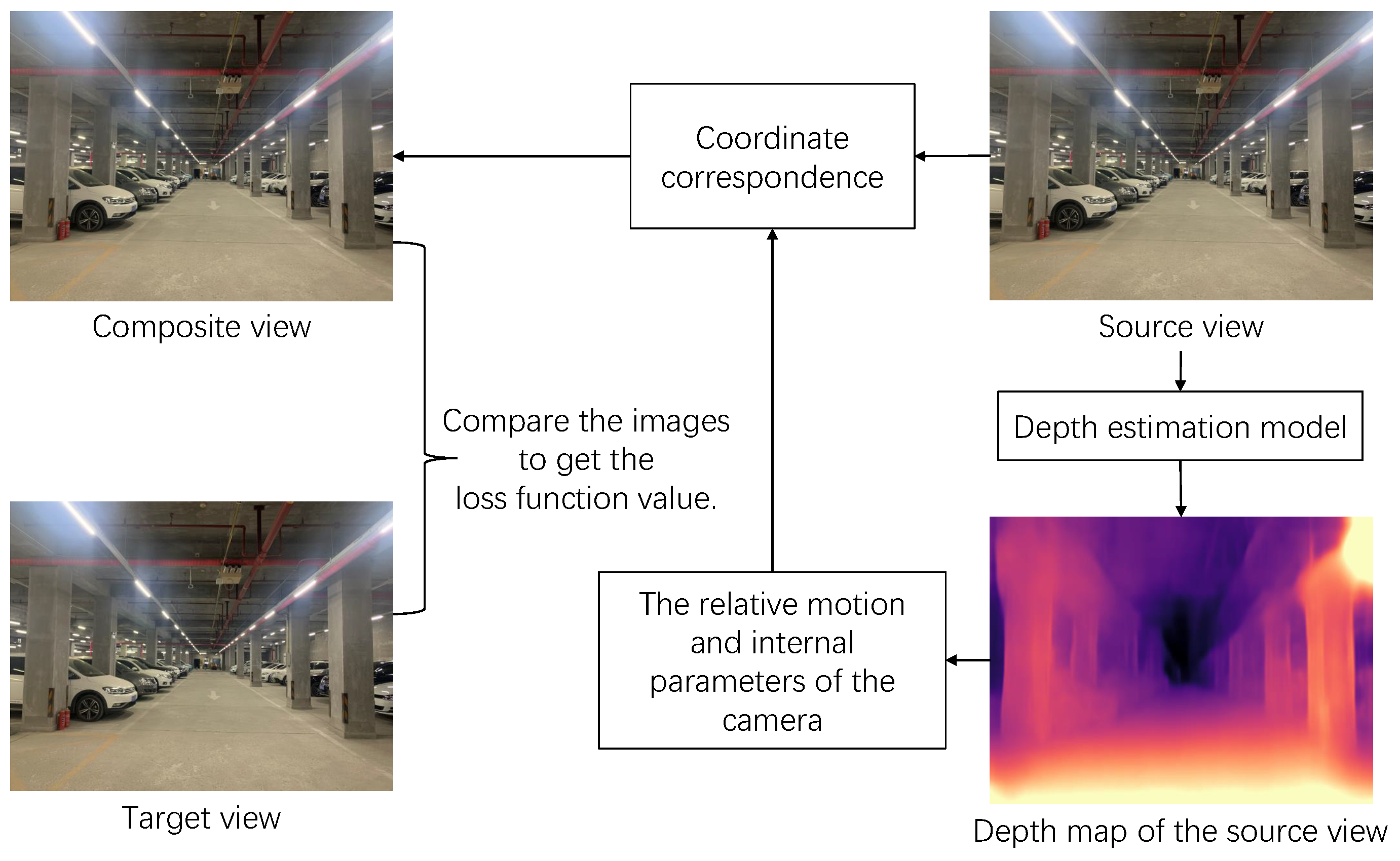
The view synthesis process is shown in Figure 1. First, we specify an image as the target view, and the other images as the source view. The depth information of the source view is obtained through the depth prediction model, and then the pixel correspondence to the target view is calculated according to the camera motion and camera internal parameters. Next, we use the source view as input to obtain the composite view of the synthesized target image. Finally, the pixel difference between the target view and the composite view is used as the loss function of the deep learning model. During our experiment, the training video is treated as a collection of RGB images $\{I_1,I_2,\dots ,I_N\}$, one of them serves as the target view $I_t$, and the rest serves as the source view $I_s(1\le s\le N,s\ne t)$.

The composite view is represented as:

$${\mathcal{L}}_{vs}=\sum _s\sum _p\left|I_t\left(p\right)-{\widehat{I}}_s\left(p\right)\right|$$

(1)

In this equation, p refers to the pixel in the image, and ${\widehat{I}}_s$ comes from the source view $I_s$. After $I_s$ passes the depth prediction model and generates the depth map, according to the camera’s internal parameters and camera motion process, it is converted to the composite view under the coordinate system of the target view. Such a transformation is based on a depth map rendering model. ${\mathcal{L}}_{vs}$ is the difference between the two views. That is, the loss function of the deep learning model.

In addition, this is a differentiable depth map-based rendering model; thus, it can reconstruct the target view $I_t$ by sampling from the source view $I_s$ based on the depth map ${\widehat{D}}_t$ and relative position pose ${\widehat{T}}_{t\to s}$.

We further calculate the coordinates corresponding to the source view through the following equation:

$$p_s\to K{\widehat{T}}_{t\to s}{\widehat{D}}_t\left(p_t\right)K^{-1}{p}_t$$

(2)

where we use $p_t$ to represent the coordinates of one pixel in the target view, and K to represent the camera reference matrix.

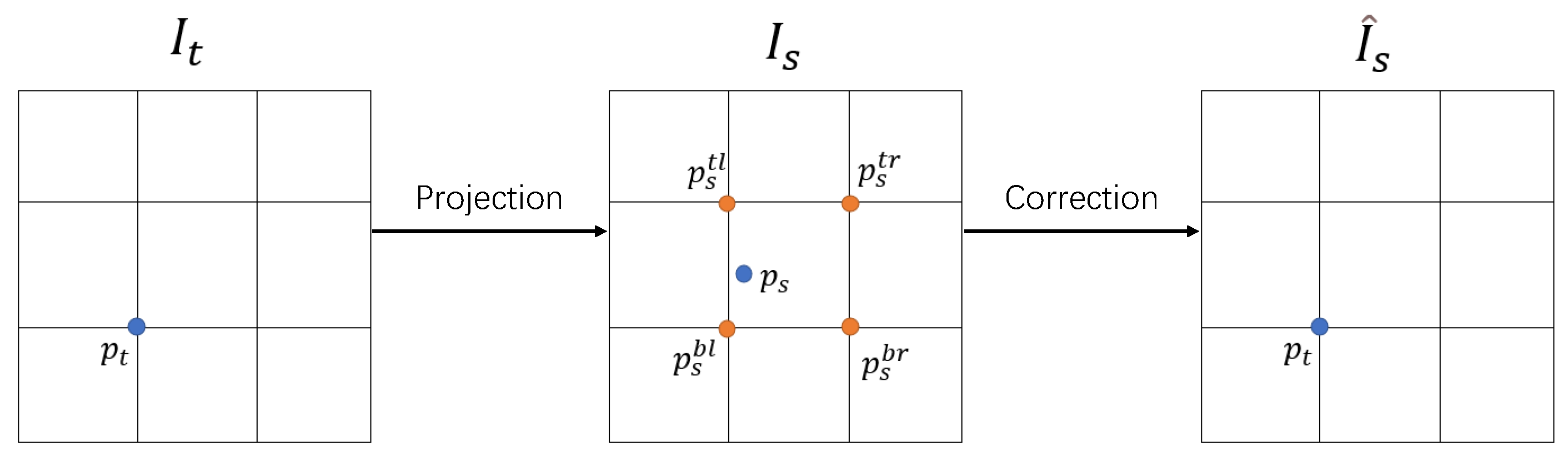
It is worth noting that the calculated $p_s$ are continuous values. Since the calculated pixel position is not necessarily an integer value and cannot be assigned directly, in order to fill the value of $I_s\left(p_s\right)$ with the value of ${\widehat{I}}_s\left(p_t\right)$ obtained, we need to adopt the following strategy. We need to obtain the RGB value of its adjacent 4 pixels (the 4 points are upper left, upper right, lower left, lower right) to approximate the pixel to be filled. The specific process is shown in Figure 2; the approximate calculation is based on the following:

$${\widehat{I}}_s\left(p_t\right)=I_s\left(p_s\right)={\Sigma }_{i\in \left\{t,b\right\},j\in \left\{l,r\right\}}{\omega }^{ij}{I}_s\left(p_s^{ij}\right)$$

(3)

In this equation, ${\omega }^{ij}$ is the linear scale of spatial proximity, and this ratio satisfies the relationship ${\sum }_{ij}{\omega }^{ij}=1$. t refers to the top, b refers to the bottom, l refers to the left, and r refers to the right.

The above deep learning model is based on three premises. First, all scenes are static and there are no moving objects. Second, in all target and source views, there is no occlusion and unblocking process. Finally, all surfaces are Lambertian surfaces. In view of the above premises, this paper proposes a supplementary term for the loss function in view composition, i.e., the geometric consistency loss. It breaks through the limitations of synthesis technology and optimize the existing model.

We use the geometric consistency of objects to constraint the depth estimated in all scenes. Precisely, we require minimal difference between $D_a$ and $D_b$ from the same object. This not only maintains geometric consistency between samples, but also the entire video sequence. With such a limitation, the depth inconsistency $D_{diff}$ is calculated for any frame of the video:

$$D_{diff}\left(p\right)=\frac{\left|D_b^a\left(p\right)-D_b^{\prime }\left(p\right)\right|}{D_b^a\left(p\right)+D_b^{\prime }\left(p\right)}$$

(4)

where $D_b^a$ is the depth map of $I_b$ calculated by using the distortion $D_a$ of the relative position pose $P_{ab}$ between A and B time slots. $D_b^{\prime }$ is a depth map interpolated from the estimated depth map $D_b$. Their differences are normalized by the sum value. This is more intuitive than using absolute distance because it treats points of different absolute depths equally in optimization. In addition, the function is symmetric and the output is naturally between 0 and 1, which contributes to numerical stability in training. With such a deep inconsistency $D_{diff}$, we define the geometric consistency loss as:

$$L_{GC}=\frac{1}{\left|V\right|}\sum _{p\in V}{D}_{diff}\left(p\right)$$

(5)

Note that our loss function with view synthesis technology is self-supervised. We take the geometric consistency loss as a supplement to the loss value calculation, and redesigns the loss computation process. In practice, minimizing the depth of predictions between each successive pair makes them geometrically consistent.

4. 3D Point Cloud Conversion

This paper proposes a method of converting a single depth map into a point cloud array and presenting it as a three-dimensional model, which have the advantage of being intuitive and figurative. We generate a point cloud array through the following three steps. First, calibrate the camera parameters to obtain the parameters of the camera. Then, we calculate 3D coordinates of each point in the point cloud map according to the camera’s internal parameters, images’ color information, and depth information. Finally, we output the point cloud with color.

Calibrate the camera parameters is a process of converting from the world coordinate system to the camera coordinate system, and ultimately to the image coordinate system. Among the above systems, the world coordinate system is of three-dimensional space, which is used to describe the specific position of objects in the real world. The camera coordinate system is established based on the camera, which is used to describe the position of the object in the camera perspective. The image coordinate system is the coordinate system of the pixel on the image, which is used to describe the position of the pixel.

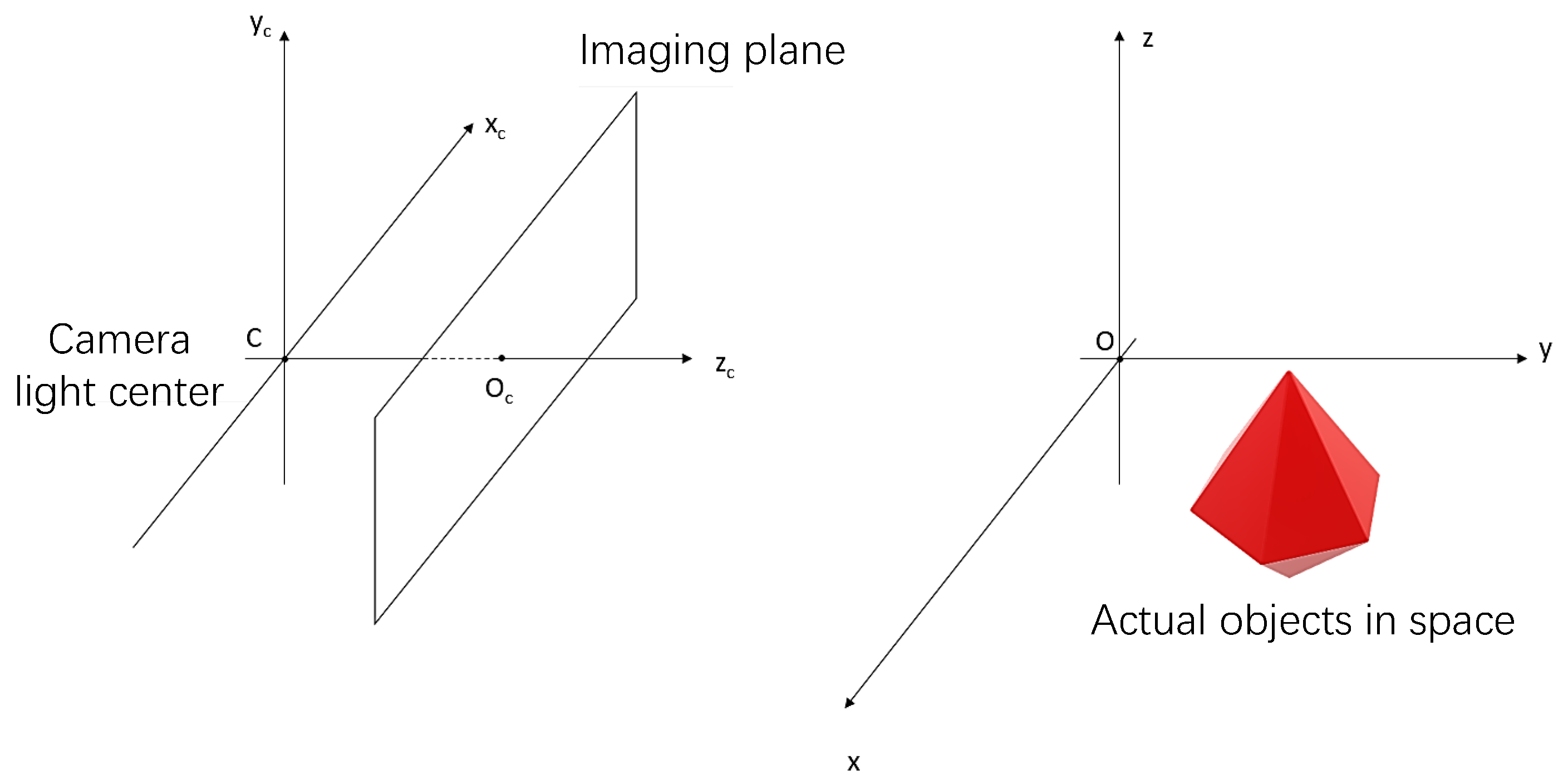
As shown in the Figure 3 below, the camera coordinate system is on the left while the world coordinate system is on the right. We first transform the three-dimensional drawing into the camera coordinate system by translation and rotation, where the rotation matrix R and the translation vector t are the external parameters of the camera. The center C of the camera coordinate system is the optical center of the camera, and the imaging plane of the camera is parallel to the $x_{c}C{y}_c$ plane and in the positive direction of the $z_c$. 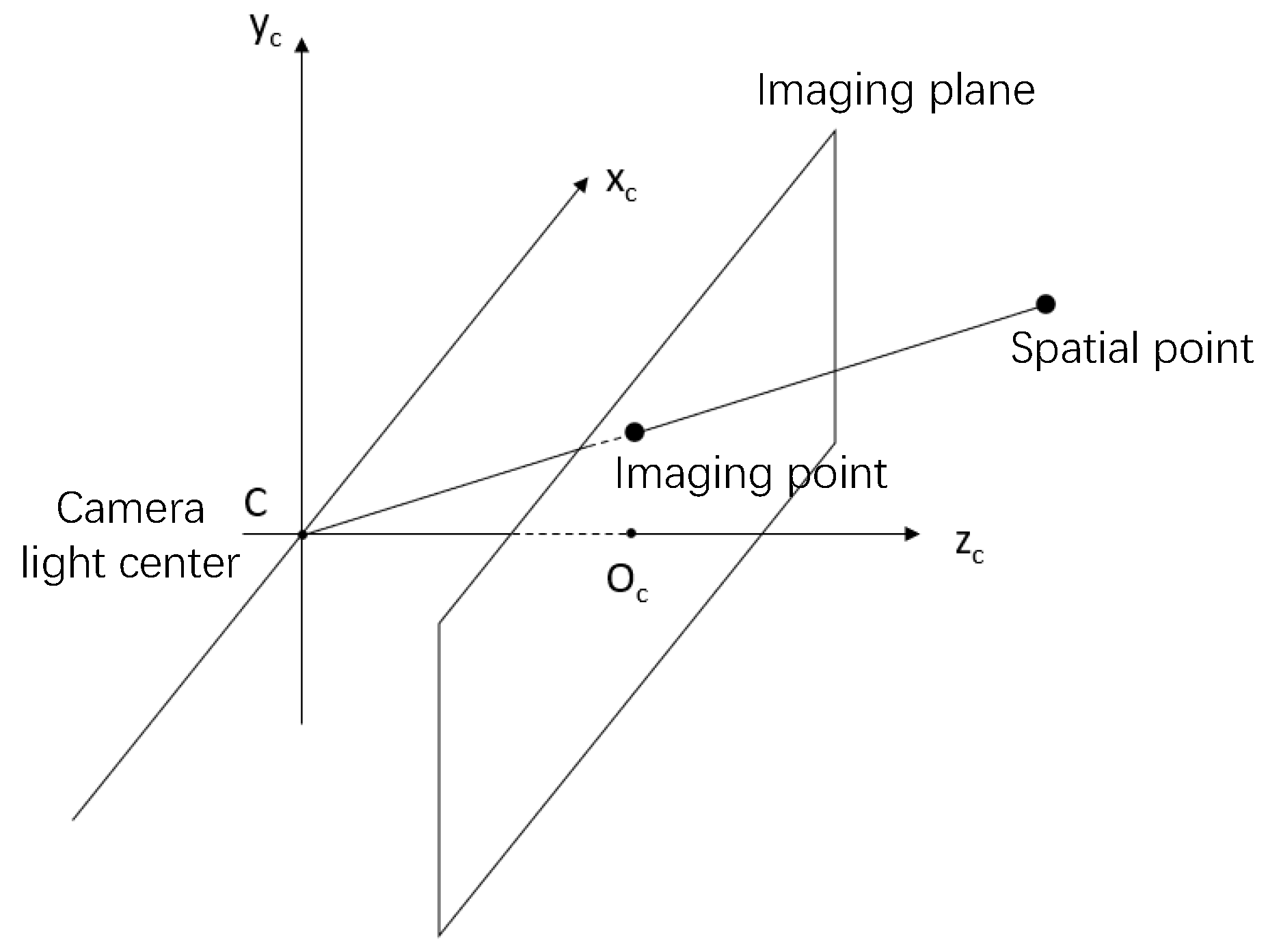The intersection point of the imaging plane and the $z_c$ is $O_c$ the main image point, and then the point in the camera coordinate system and the camera light center are connected. The intersection point of the connection and the imaging plane is the image formed by the point in the camera, as shown in the Figure 4 below.

In general, the camera’s internal parameter matrix K is as follows:

$$K=\left[\begin{array}{ccc}{f}_x& s& c_x\\ 0& f_y& c_y\\ 0& 0& 1\end{array}\right]$$

(6)

where $f_x$ and $f_y$ is the focal length of the camera in the x and y directions, $(c_x,c_y)$ is the coordinate of the main image point, and s is the tilt parameter of the coordinate axis, which is ideally 0.

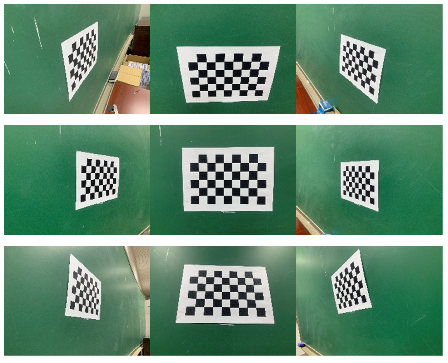
The input for camera calibration is the image coordinates of all interior corner points on the calibration image, and the three-dimensional spatial coordinates of all inside corner points on the calibration image, where the default image is on the plane of $z=0$. The output of the camera calibration is a matrix of internal and external parameters of the camera.

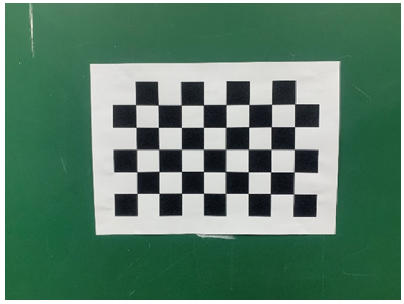
In order to complete the calibration of the internal parameters of the camera, a camera parameter calibration plate with a black and white grid needs to be prepared. The process of parameter calibration is as follows:

• Set parameters for finding sub-pixel corners.
• Build an array to store the position coordinates of each corner point, each coordinate contains $(x,y,z)$ data.
• Define that the calibration plate is located on the $z=0$ plane, so the z-coordinate of all points is 0. Assign a value to the x, y coordinates of each point in a black and white grid length, for example, the point coordinates of the first row are:

  $$(0,0,0),(1,0,0),(2,0,0),...,(8,0,0).$$
• Read all captured pictures and find all sub-pixel corners.
• Enter the data in the above steps as parameters, and call the function of OpenCV2 to calibrate the camera parameters.

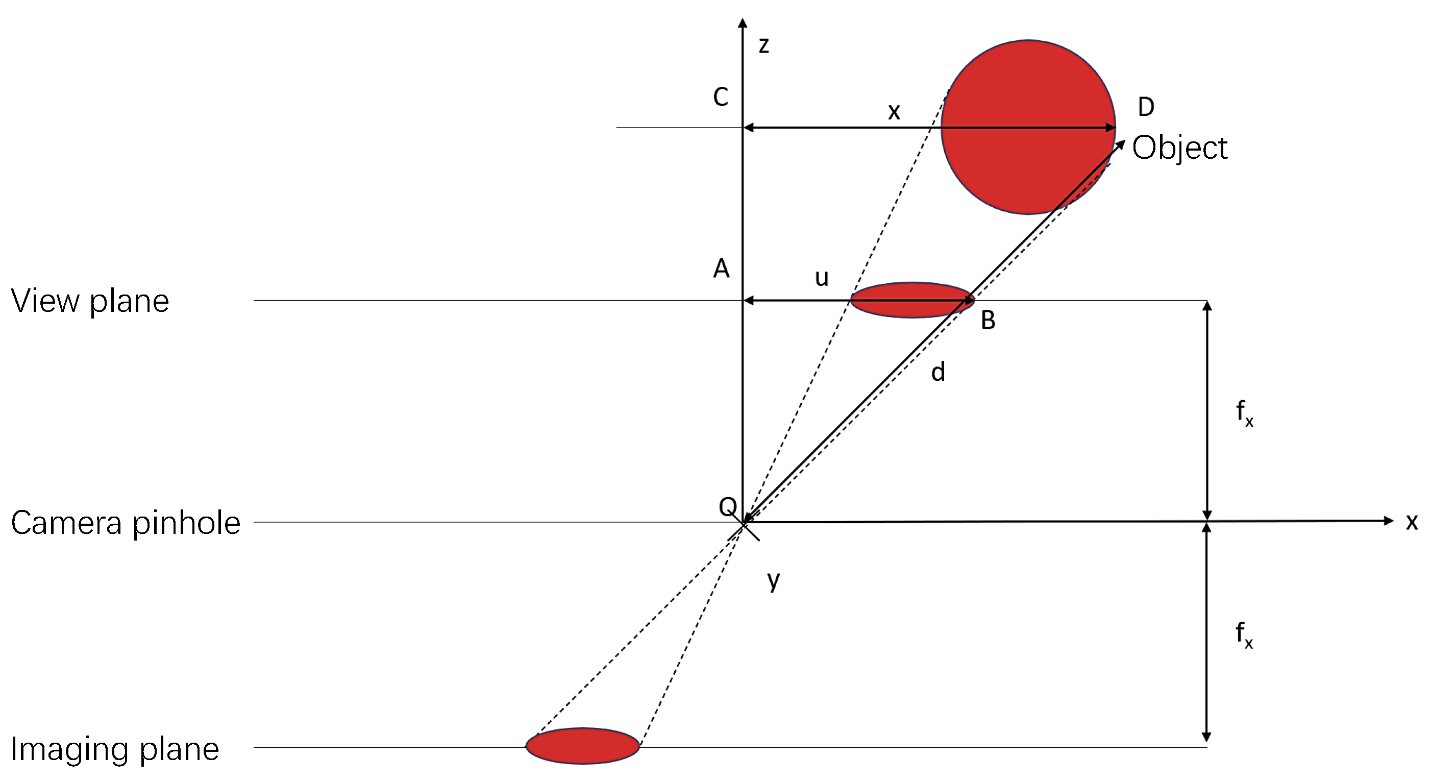
With the camera’s parameters acquired, three-dimensional modeling can be performed in combination with depth information. The core task of 3D modeling is to clarify the conversion relationship between RGB images and the 3D coordinates of the scene; thus, we need to study the camera properties. The figure below reflects the imaging principle of the camera.

As shown in the Figure 5, suppose there is an object in front of the camera, which is displayed as a projection of the $xOz$ plane in the form of a top view. On the left, there is a pinhole camera that displays the object in front of the camera on the screen. The world coordinate system is aligned with the camera, so the z axis extends to the direction the camera sees. The world coordinate system is aligned with the camera, so the z axis extends to the direction the camera sees. Point D of the object is point B in the image created by the camera. The horizontal coordinate of D is x, and the corresponding horizontal pixel coordinate of B on the image is u. The y-axis is the same, the vertical coordinate of D is y, and the corresponding vertical pixel coordinate of B on the image is v. In ordinary RGB images, there is no embodiment of the information of the z-axis coordinate of point D, so depth information d is also essential in the work of three-dimensional coordinate reconstruction. There are many references when estimating depth, the most important of which is the focal length, which marks how pixel coordinates are converted to length, which is the actual distance between the lens and the film or sensor.

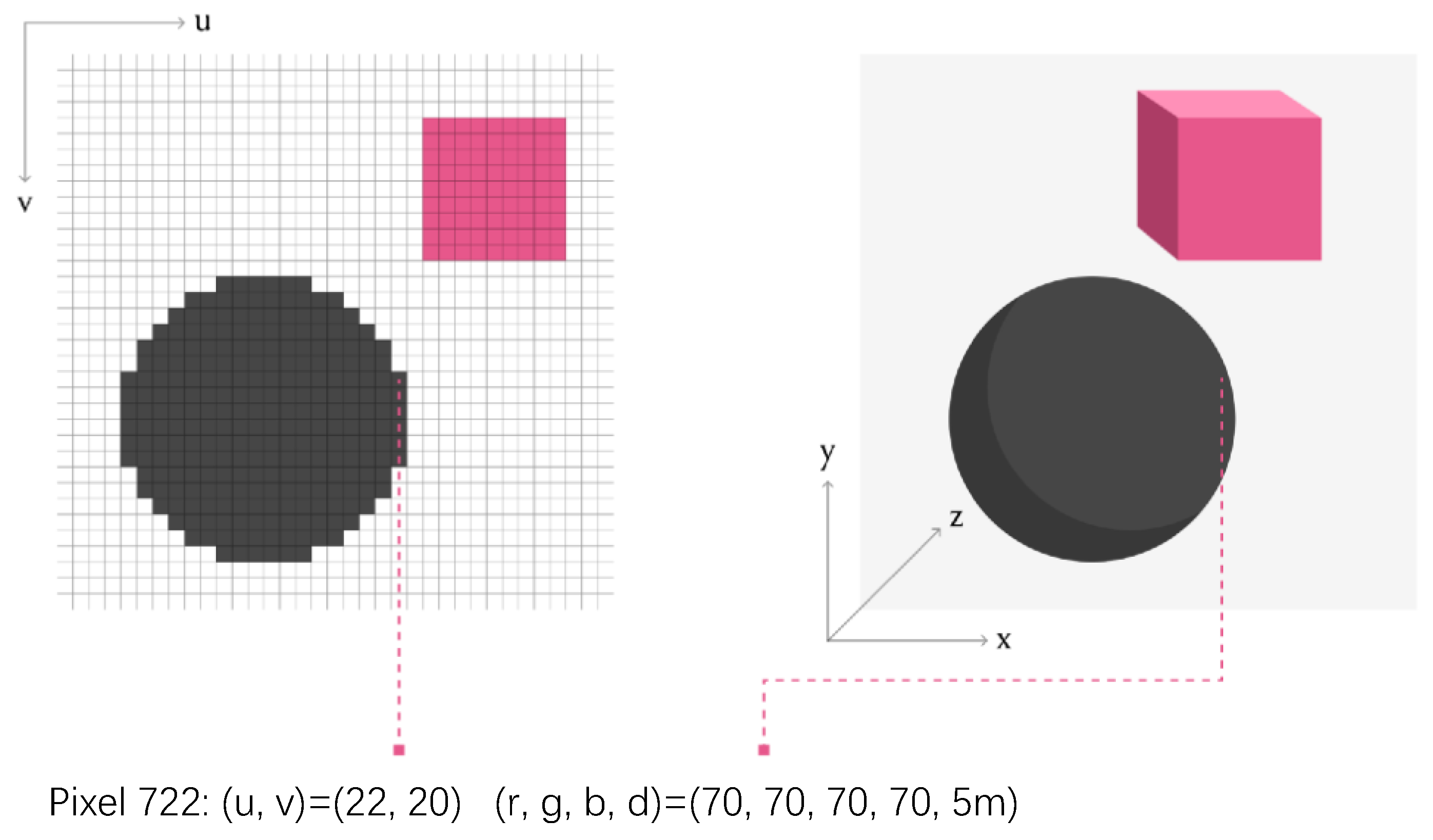
So far, we have preliminarily clarified the conversion relationship from the world coordinate system to the camera coordinate system. In order to further explore the transformation of the camera coordinate system to the world coordinate system, an RGB map and the corresponding depth map are introduced for analysis.

As shown in the Figure 6, on the left is a two-dimensional plan, take the sample point with pixel coordinates $(u,v)$, each pixel has an RGB color value and corresponding depth. On the right is a schematic of two objects in a three-dimensional coordinate system. Depending on the imaging principle of the camera, the position x can be easily derived from the lateral pixel coordinates u and depth information d of each pixel. In addition, do the same for y and v. It should be noted that for pinhole camera models, the focal length in the x and y directions is the same, but this is not always the case in reality for cameras with lenses, so the focal length in the x and y directions needs to be calibrated when parameterizing in the camera. Only then can the correct coordinate calculation be carried out. It is not difficult to calculate the corresponding relationship between pixel coordinates and three-dimensional spatial coordinates as follows:

$${(x,y,z)}^T=z{\left[R|t\right]}^{-1}{K}^{-1}{(u,v,1)}^T$$

(7)

where $K$ is the camera’s internal parameter matrix, $\left[\left.R\right|t\right]$ is the camera’s external parameter matrix, R is the rotation matrix, and $t$ is the translation vector.

The specific process of this module is as follows:

• Input RGB diagram, depth map, depth map scale factor, camera internal parameter matrix K and camera external parameter matrix.
• Create an array of floating-point numbers u, and a shape [1] of length RGB matrix.
• Create an array of floating-point numbers v, and a shape [0] of length RGB matrix.
• Default camera coordinate system as the world coordinate system. Create an array of point clouds that store the coordinates $(x,y,z)$ and color data $(R,G,B)$ for each point. The array length is shape [1] × shape [0] of the RGB matrix. That is, each pixel corresponds to a point in the point cloud.
• Iterate through each pixel.
• According to the formula above, the coordinates corresponding to each pixel are generated, and the values of $R,G$, and B are maintained for the $R,G,B$ values of the pixels.
• Save the point cloud array as a “.ply” file.

The rgb entered in the code is an RGB image, consisting of a two-dimensional matrix of elements as tuples of $(R,G,B)$. Depth map is composed of a two-dimensional matrix based on the depth information of a single point. Depth map scale factor may be different for different cameras, such as the scale factor of the camera used in the common TUM dataset is 5000. Since the depth map in this paper is not obtained by the depth camera, but by the depth prediction deep learning network, there is no camera parameter that can be referenced, and this parameter needs to be manually calibrated. This scale factor is the ratio of the values stored in the depth map to the true depth.

K is the 3 × 3 camera internal parameter matrix, and camera external parameter matrix is the transformation matrix of 4 × 4 under the Cartesian coordinate system of the camera coordinate system to the world coordinate system. If no external parameter matrix is entered, then the matrix defaults to:

$$\left[\begin{array}{cccc}1& 0& 0& 0\\ 0& 1& 0& 0\\ 0& 0& 1& 0\\ 0& 0& 0& 1\end{array}\right]$$

(8)

So far, we have obtained the array of point clouds corresponding to the RGB color image. Next, the array of point clouds is stitched together into a 3D model. In this paper, the ICP (Iterative Closest Point) algorithm is used for implementation. Considering the differences between real scenarios and ideal scenarios, the basic ideas of algorithms discussed in this article will be divided into reasoning in ideal situations and methods for applying them to real situations. First, we discuss the reasoning of ideal situation. Suppose that the two point cloud arrays entered are P and Q, where: $P=\left\{p_1,p_2,p_3,\dots ,p_N\right\}$, $Q=\left\{q_1,q_2,q_3,\dots ,q_N\right\}$.

$p_i$ and $q_i$ are the points in the point cloud, $i\in \left[1,N\right]$.

There is a set of correspondences between the points in these two point clouds: $C=\left\{\left(i,j\right)\right\}$

Such a correspondence indicates that the point cloud $p_i$ from P corresponds to the point cloud $q_i$ from Q. The output of the ICP algorithm is a translation vector t and a rotation matrix R, satisfying that the difference between the two point clouds is minimized after this translation and rotation on the point cloud P. This difference is calculated by the following formula:

$$E\left(R,t\right)=\sum _{(i,j)\in C}\left|\right|q_i-R{p}_j-t{\left|\right|}^2$$

(9)

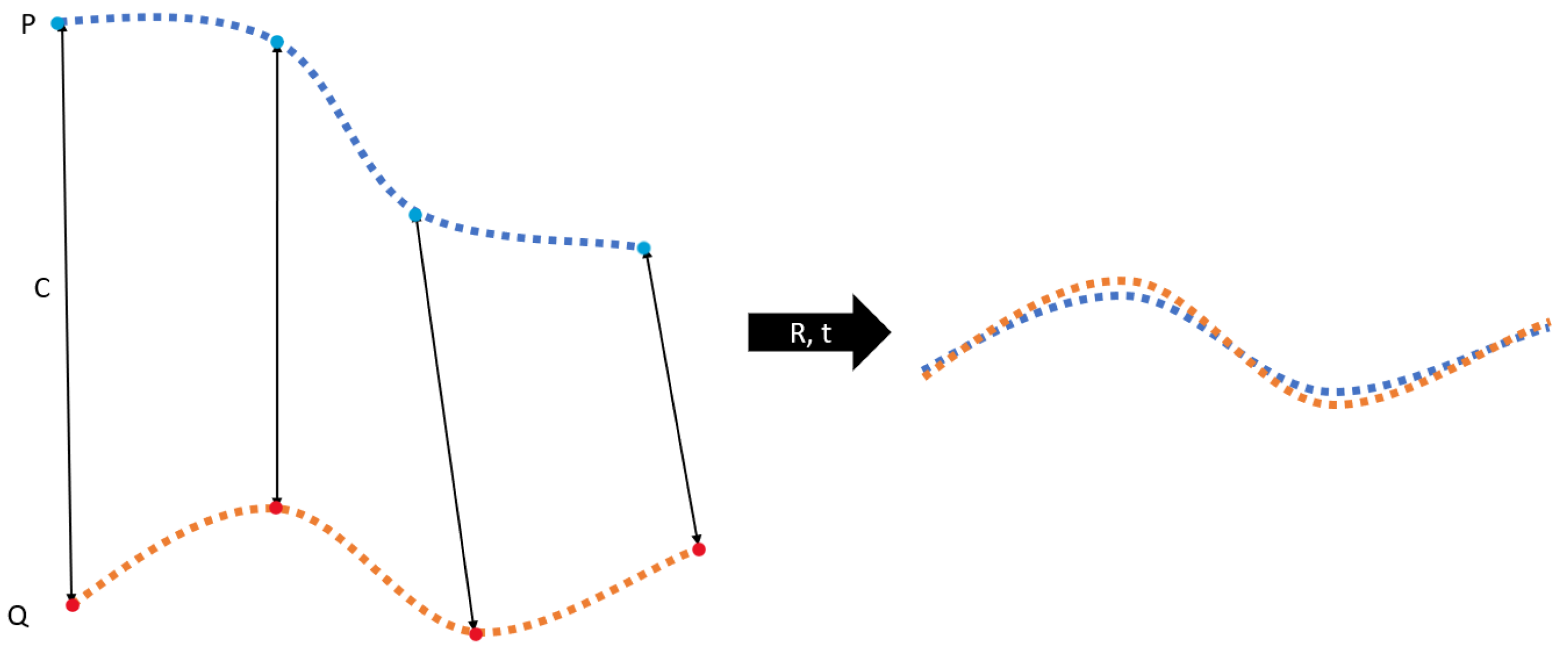
The core idea of ICP is that assuming that we know the correspondence C between point cloud P and point cloud Q, and assuming that this relationship is correct, then ICP needs to minimize the sum of distances between the corresponding points through the rotation and translation operation of the point cloud P, as shown in the following Figure 7:

The blue part on the left side of the figure is the point cloud P, the red part is the point cloud Q, and the black double-headed arrow indicates the correspondence between the points in the point cloud. After the point cloud P is translated $\left(t\right)$ and rotated $\left(R\right)$, the resultant point cloud is shown on the right side of the figure. The ICP algorithm calculates such a rotation matrix R and translation vectort based on the coordinates of the points in the point cloud P and Q, and the correspondence C.

The method is to first calculate the center of gravity of the two point clouds, and then subtract the geometric center coordinate of P from the geometric center coordinate of Q, and the resulting vector is the translation vector t, and after such a translation of P, the geometric center of the two will overlap. The calculation formula is:

$${\mu }_Q=\frac{1}{\left|C\right|}\sum _{\left(i,j\right)\in C}{q}_i$$

(10)

$${\mu }_P=\frac{1}{\left|C\right|}\sum _{\left(i,j\right)\in C}{p}_j$$

(11)

where the center of gravity of P and the center of gravity of point cloud Q are ${\mu }_P$ and ${\mu }_Q$. $\left|C\right|$ indicates the number of point pairs in the corresponding relationship.

Next, two new point clouds $P^{\prime }$ and $Q^{\prime }$ can be generated, with the same center of gravity at the same point. The resulting method is to subtract the corresponding center of gravity coordinates for each point in point cloud P and point cloud Q, and the calculation formula is:

$$Q^{\prime }=\left\{q_i-{\mu }_Q\right\}=q_i^{\prime }$$

(12)

$$P^{\prime }=\left\{p_j-{\mu }_P\right\}=p_j^{\prime }$$

(13)

Therefore, the expression of the original error function becomes the following expression, in which case the error function is only related to the rotation matrix, satisfying the following expression:

$$E^{\prime }\left(R\right)=\left|\right|\left[q_1^{\prime }\cdots q_n^{\prime }\right]-R\left[p_1^{\prime }\cdots p_n^{\prime }\right]{\left|\right|}_F^2$$

(14)

Solving such a matrix R is called an orthogonal procrustes problem, and such a problem can be solved by singular value decomposition. The solution process of matrix R is as follows:

First, calculate the cross covariance matrix:

$$W=\sum _{\left(i_{j}j\right)\in C}{q}_i^{\prime }{p}_j^{\prime T}$$

(15)

Next, the transpose of the matrix U and D matrices is obtained using singular value decomposition. In addition, obtain the transpose of the V matrix:

$$W=UD{V}^T$$

(16)

where U, V is the rotation matrix of 3 × 3. D is the diagonal matrix.

Finally, the rotation matrix R is calculated using U, V:

$$R=U{V}^T$$

(17)

$$t={\mu }_Q-R{\mu }_P$$

(18)

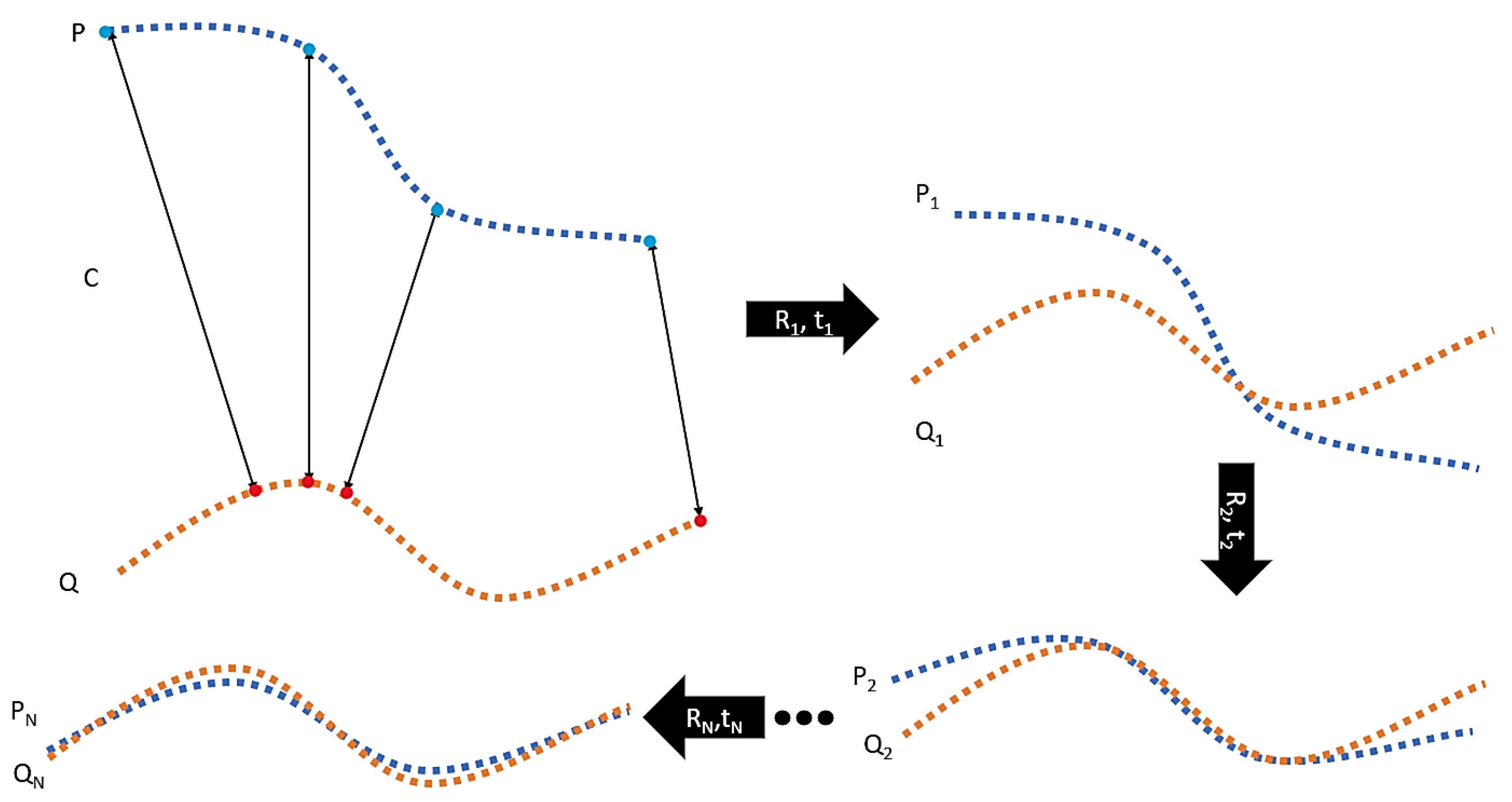
From the above calculation, we can obtain the rotation matrix R and the translation vector t. However, this is in the ideal situation of knowing the correspondence C in point cloud P and point cloud Q, but in reality there is often no such correspondence C. The ICP algorithm needs to iterate to find its correspondence. It is basically impossible to find the rotation matrix R and the translation matrix t in one step, ICP will guess such a correspondence $C_1$, and then use this correspondence to calculate the $R_1$, $t_1$ and apply it to the point cloud P to obtain the $P_1$, and then do the same for $P_1$ and Q, and so on. The more iterations, the smaller the error function.

Take the following Figure 8 as an example of two point clouds:

The blue point cloud P and the red point cloud Q have no corresponding relationship C. We assume that the point on Q corresponding to a point on P is the point on Q closest to that point. Thus, the correspondence $C_1$ is established, through $C_1$ which $R_1$ and $t_1$ can be calculated, and such translations and rotations can be applied. Obtain new point cloud $P_1$ and $Q_1$. This operation is repeated until the error function of the two is small enough to obtain a spliced point cloud.

In this paper, the coordinate system transformation relationship under different coordinate systems is combined with independent experiments on cameras to obtain the internal and external parameter information of cameras. We adopt the imaging principle of the camera and the parameters of the camera to reconstruct the 3D scene of the depth map, and extracts the color value of each pixel from the RGB map to color the 3D model, and finally converts the video stream into a 3D model, making the results of depth estimation more intuitive and facilitates analysis.

5. Evaluation

5.1. Experimental Equipment and Dataset Acquisition Process

Prototype. We developed a smart vehicle prototype with a monocular camera (an Astra Camera with 25 fps) to capture images, and produce depth maps and 3D point cloud with network/server support, as shown in the following Figure 9.

5.2. Sub-Module Evaluation

Depth estimation. This paper applies the deep learning network to the underground parking lot environment and corridor environment. In order to better observe the results of the depth map, we use the “magma” coloring scheme to color the depth map and output it as an RGB image to visualize the depth information. The depth chart effect is shown in the following Figure 10.

3D modeling. In order to calibrate the camera parameters, we print a 9 × 6 black-and-white grid diagram with an inner corner point of 8 × 5 checkerboard, and each grid size is 27 mm × 27 mm. As shown in the following Figure 11.

We put it on a flat surface and use the monocular camera to shoot it at different angles. We divide them into upper left, upper center, upper right, middle left, center, middle right, bottom left, bottom left, bottom center, and bottom right. A total of 18 pictures are taken, as shown in the Figure 12 below.

The calibrated camera internal parameter matrix is shown as:

$$\left[\begin{array}{ccc}3.1081\times {10}^3& 0& 0\\ 0& 3.1056\times {10}^3& 0\\ 2.0061\times {10}^3& 1.4759\times {10}^3& 1\end{array}\right]$$

(19)

Next, we input depth map and original map to produce the point cloud. During the conversion process, the internal parameters of the camera are used as parameters to calculate the x and y coordinate information of the pixels. We use pixel depth to determine the z-coordinate information of the pixel. The depth map provides the three-dimensional coordinate information of a certain pixel, and the original image provides the RGB color information of the point to complete the conversion. Finally, we apply Meshlab and open3D to recognition, and the transformation effect is shown in the Figure 13:

5.3. Evaluation Indicators

Since the result point cloud of 3D modeling is generated strictly according to the depth map, the test point of the mapping technique used in this paper is the accuracy of the depth map. We use the measured depth data of the meter scale as the truth value and compare it with the depth map generated in this article. The following parameters are used as evaluation criteria.

Error:

$$\frac{y_1}{y_1^{*}}·y_2-y_2^{*}$$

(20)

Average of errors:

$$m=\frac{1}{N}·\sum _{pic}(\frac{y_1}{y_1^{*}}·y_2-y_2^{*})$$

(21)

Variance of error:

$${\sigma }^2=\frac{1}{N}·\sum _{pic}{(\frac{y_1}{y_1^{*}}·y_2-y_2^{*}-m)}^2$$

(22)

Standard deviation of error:

$$\sigma =\sqrt{\frac{1}{N}·{\sum }_{pic}{(\frac{y_1}{y_1^{*}}·y_2-y_2^{*}-m)}^2}$$

(23)

where $y_1$ is the length of a distance in the scene in the image format, and $y_1^{*}$ is the length of the same distance in the real scene. $y_2$ and $y_2^{*}$ are the length of another distance of the same image in the image format and the length in the real scene. $pic$ is the test gallery and N is the total number of images in the test gallery.

5.4. Quantitative Evaluation

This article uses 17 images as samples for testing, of which 8 belong to the parking lot scene and 9 belong to the corridor scene. The test results are shown in

Table 1. Depth estimation error.

Test Environment	Image Index	Error (cm)
parking lot	1	23.63
parking lot	2	10.81
parking lot	3	27.74
parking lot	4	15.01
parking lot	5	15.67
parking lot	6	8.08
parking lot	7	7.45
corridor	1	13.14
corridor	2	4.79
corridor	3	10.00
corridor	4	0.10
corridor	5	10.77
corridor	6	9.58
corridor	7	8.19
corridor	8	7.03
corridor	9	4.99
corridor	10	2.48
Average error		10.56
Variance error ${\sigma }^{\mathbf{2}}$		46.65
Standard deviation error $\sigma$		6.83

.

6. Conclusions

In this paper, we propose a monocular depth estimation algorithm to improve the robustness and deployment of autonomous driving. We used a simple monocular camera to predict the scene depth information and generate the 3D map. This work can be carried on lightweight mobile intelligent systems, and the results prove the effectiveness of our system.