Knowledge-Based Features for Speech Analysis and Classification: Pronunciation Diagnoses

Abstract

Accurate pronunciation of speech sounds is essential in communication. As children learn their native language, they refine the movements necessary for intelligible speech. While there is variability in the order of acquisition of speech sounds, there are some sounds that are more complex and are later developing. The rhotic /r/ is a later-developing sound in English, and some children require intervention to achieve accurate production. Additionally, individuals learning English as a second language may have difficulty learning accurate /r/ production, especially if their native language does not have an /r/, or the /r/ they produce is at a different place of articulation. The goal of this research is to provide a novel approach on how a knowledge-based intelligence program can provide immediate feedback on the accuracy of productions. In the proposed approach, the audio signals will first be detected, after which features of audio signals will be extracted, and finally, knowledge-based intelligent classification will be performed. Based on the obtained knowledge and application scenarios, novel features are proposed and used to classify various speaker scenarios.

1. Introduction of English Pronunciation

1.1. Native Speakers and Second Language Speakers

Typically, native speakers of a language can quickly identify second language learners due to variations in the stress patterns and prosody of speech and the articulation of individual sounds [1]. These variations occur because the language learner must overcome interference patterns from their first language. In addition to learning which syllable must be stressed in a word, the learner must refine and create additional phonemic categories, focusing on acoustic characteristics of sounds that may not have been distinctive in their first language. Once the learner can hear the acoustic differences between the new phonemes, they must determine the articulatory placements required to pronounce them. This is not an easy task, and characteristics of the native and second language can make it even more difficult. A study indicates that it is challenging to change the accent of non-standard English speakers, even after engaging in a 10-month full-time English class [2]. Further, not all phonemes are created equally, with some being more frequent cross-linguistically, making them easier for language learners to incorporate in their speech. Other phonemes may be articulatorily complex or may be acoustically very similar to or distinct from other sounds in their native phonetic inventory, making them more challenging to incorporate in their phonemic repertoire [3].

1.2. Method to Pronounce Phonetic /r/

In English, there are two main methods to produce the /r/, and while the location of the tongue is very different between the two, the resulting sound is similar. One method of production is referred to as bunched. The back of the tongue is lifted, thereby putting the sides of the tongue in line with the back teeth. The middle of the tongue’s back is lower and the air flows to build the resonance across this groove. The tip of the tongue will point upwards or stay down. The second method is considered a retroflex. The tip of the tongue is elevated and curves backward behind the tooth ridge while the back of the tongue remains low [4].

When it comes to Asian languages, pronunciation of the English /r/ is challenging because /r/ is not common in these languages. For example, in Japanese, there are five characters in the Romanization of Japanese “ra, ri, ru, re, ro.” In Japanese, /r/ and /l/ are allophones in free variation, meaning they can be substituted with each other without changing the meaning of the words. Thus, Japanese speakers do not need to focus on the acoustic distinctions between /r/ and /l/ because they are not distinct phonemic categories; /li/ and /ri/ can both be understood as “ri.” When Japanese speakers learn English, they are challenged to reconfigure their underlying representations of sound categories and differentiate /r/ and /l/ when speaking English and ignore the distinction when speaking Japanese. The complexity of production and many phonetic contexts of the American English /r/ make accurate production challenging even after years of speaking English.

1.3. Speech and Language Disorder and Assessment

Speech disorders can affect pronunciation, which influences their everyday lives. While distortion errors may not affect the understanding of speech as severely as omission or substitution, it does not mean distortion errors should be ignored, because they can result in negative academic [5] as well as emotional and social consequences in children [6,7].

Further, while the cause of the delay is not always known, there are other diagnoses that indicate intervention is necessary before the child even starts to speak. For example, children with hearing loss are deprived from the acoustic signal. Without amplification, they will have extreme difficulty creating the phonemic categories of their language. Thus, early intervention is critical [8].

Because some children with speech sound errors also have a language impairment [9], diagnosis of a speech sound disorder typically occurs after a comprehensive speech-language evaluation. The evaluation will consist of a hearing test and an oral-peripheral test to rule out organic causes for the speech errors. A variety of standardized assessments will be utilized to test the child’s understanding and use all of the domains of language: semantics (vocabulary), syntax (word order), morphology (base words, prefixes, and suffixes), phonology (sound system) and pragmatics (social communication). A conversational speech sample will allow for voice and fluency to be screened as well as additional conversational speech-language analyses to be completed. Common articulation and phonology measures extracted from the conversational speech-language sample are phonetic and syllable inventories, as well as a calculation of percent consonants correct (PCC). An important component of all speech sound evaluations is stimulability testing, which will indicate if the individual has the capacity to produce the sound with perceptual, instructional, or tactile cueing [10].

1.4. Purpose and Proposed Work

The current project aims to evaluate the effectiveness of using signal processing and pattern recognition in remediating /r/ mispronunciation. A crucial aspect of addressing /r/ errors is training individuals to perceptually distinguish between correct and incorrect productions. Once individuals can differentiate between the two, they can start modifying their tongue movements to approximate accurate /r/ pronunciation. Speech-language pathologists play a crucial role in guiding individuals on how to move their tongue correctly and provide feedback on the accuracy of their production. They may also assign homework to facilitate practice and reinforce new motor movements. However, practice may prove counterproductive if the speaker continues to produce the sound incorrectly, thereby increasing the habitual nature of the distorted sound.

To address this challenge, a pronunciation analysis and classification system is proposed to provide individuals with immediate feedback on their productions, enabling them to identify inaccuracies and make necessary modifications. In this project, we propose using speech signal processing, analysis, and pattern recognition techniques to classify pronunciation accuracy. We plan to use /r/ as the pilot study to demonstrate the feasibility of using advanced signal processing and pattern recognition approaches to improve speech production.

Similar to automatic speech recognition (ASR), the proposed analyzing/classifying system includes speech detection, pattern or feature extraction, and classification parts. However, the objective of ASR is to figure out the contents embedded in the speech waveform, whereas the purpose of this study is to identify correct and incorrect pronunciation. Therefore, the typical features used for ASR cannot be directly used without modification. To address this issue, we propose engineering new features for this task.

The mechanism for generating speech in humans involves a complex interaction between various biological structures, including the lungs, larynx, vocal cords, and articulators. The process begins when air is exhaled from the lungs and passes through the larynx, where it causes the vocal cords to vibrate when producing voiced sounds. These vibrations produce a sound wave that travels up the throat and into the mouth (and nose for nasal sounds), where it is shaped into speech sounds by the movement of the tongue, lips, and other articulators. Different speech sounds are created by manipulating the shape of the vocal tract. The movement of the articulators create different filters that modify the sound wave. In order to capture the collaboration and the changes of those structures. We propose the Pitch and Partials Amplitude Gradient (PPAG) feature, which tracks the changes in the fundamental frequency and its harmonics in their magnitude, capturing the subtle variations in the process of speech sound production.

Achieving correct pronunciation requires the precise collaboration of all the biological systems in time and space, resulting in the production of an accurate acoustic waveform. In contrast, incorrect pronunciation arises from errors in one or more of these systems, or from incorrect collaboration among them, resulting in the production of an inaccurate waveform. Incorrect wave forms can differ from one another in terms of their position, momentum, and energy, and are characterized by different probabilities. In contrast, correct wave forms are similar to one another and are produced with greater probability when all the biological systems are properly calibrated and functioning together. These observations suggest that the production of speech may be best understood as a complex quantum mechanical process, where the correct pronunciation corresponds to the quantum state with the highest probability, resulting from the coherent interaction of multiple physical systems. To explore this hypothesis further, we propose borrowing the concept of the Schrödinger equation to model the phenomenon of speech production. We designed the second innovative feature, a speech wave function-based probability amplitude (SWPA) feature from speech signals.

This paper is organized as follows: Section 2 describes the speech sound detection methods; Section 3 reviews the typical features used for ASR; Section 4 proposes innovative features based on calculating the gradients of the pitch, its partials from speech signals, and SWPA features based on wave function; Section 5 presents the classifiers for recognizing the correctness of the speech signals. The experiments and results are shown in Section 6. Section 7 concludes this paper.

2. Speech Signal Detection

Speech signal processing has been a dynamic and constantly evolving field for a couple of decades now. It involves a range of techniques and methods for analyzing, manipulating, synthesizing, interpreting, and recognizing speech signals. Some of the main areas of speech signal processing include speech analysis, speech synthesis, speech coding and compression, speech enhancement, speech recognition and transcription, speaker identification and verification, and language modeling and understanding.

Speech processing has a wide range of real-world uses in diverse aspects of our everyday lives, including communications, consumer electronics, education, entertainment, and healthcare services. For example, speech recognition is used in virtual assistants, speech-to-text transcription is used for dictation and subtitling, speech processing is used in telecommunications and call centers, and speech therapy uses real-time feedback and guidance to help individuals with speech disorders. Additionally, speech processing is used in biometric identification, forensic analysis, and in education to teach foreign languages and improve pronunciation. In entertainment, speech processing is used in voice acting and dubbing, as well as creating synthetic voices for characters in movies and video games. Overall, speech processing has a broad range of applications and continues to play an increasingly important role in our daily lives as technology advances.

Speech signals are non-stationary, meaning that many algorithms designed for stationary signal processing cannot be directly applied to speech without modification. However, research has shown that for short time intervals of 10–30 milliseconds (ms) in length, speech signals can be viewed as stationary signals for certain applications [11]. Additionally, speech signals contain voiced, voiceless, and silent portions, each with different short time characteristics such as power and frequency. Therefore, speech detection and segmentation are widely used in speech signal processing.

Typically, the first step in speech signal processing is speech signal detection, followed by segmentation and other processing steps such as speech coding, feature extraction, and more.

2.1. Short-Time Energy

Short-time energy (STE) is one of the most popular methods for speech detection, as the voiced portion of speech typically has a higher STE, while the voiceless component has a significantly lower STE, and the silent portion has the lowest STE. Additionally, STE can be used to determine the beginning and ending points of each word.

STE is defined as the average of the squared values of a signal’s samples within a given window. The mathematical representation of a window may be defined as follows [12]:

$$STE=\frac{1}{N}\sum _{m=0}^{N-1}{\left[W\left(m\right)x(n-m)\right]}^2$$

(1)

where $w\left(m\right)$ is the window coefficient correspond, m is the sample index, and N is the length of a window.

A normalized STE > 0.07 was set as a threshold to remove the silent portion, such as whispering and breathing. The second threshold was set as $0.14$ seconds in duration in order to remove some impulsive voiced artifact such as a cough or sneeze.

2.2. Short-Time Magnitude

Additionally, the short-time magnitude is commonly used as a time-frequency representation for audio signals, and usually used to detect speech signals as well, particularly when a signal has a wide dynamic range. Short-time magnitude is described as follows [12]:

$$M_n=\sum _{m=-\infty }^{\infty }\left|x\left(m\right)\right|w(n-m)$$

(2)

with $\left|x\right(n\left)\right|$ denoting the signal’s magnitude,

3. General Feature Extraction for Speech Signals

Speech features refer to the characteristics of the speech signal that are extracted and analyzed to represent the speech signal in a more concise and meaningful way. These features are used in various speech processing applications such as speech recognition, speaker identification, and speech synthesis. Some commonly used abstract-based features in speech signal analysis include Linear Predictive Coding (LPC), Linear Predictive Cepstral Coefficients (LPCCs), the Mel-frequency Cepstrum Coefficient (MFCC), and Bark Frequency Cepstral Coefficients (BFCCs).

3.1. Linear Predictive Coding (LPC)

Linear predictive coding (LPC) is a common technique used for speech coding and speech recognition. It models the spectral envelope of speech using a linear predictive model and represents it in digital form [13].

A LPC algorithm computes a vector of coefficients which presents an all-pole filter [14].

$$H\left(z\right)=\frac{1}{1-{\sum }_{i=1}^M{a}_i{z}^{-i}}$$

(3)

where $a_i$ are the LPC coefficients, and M is the order of the filter.

A speech sample can be predicated by using a linear combination of the past M speech samples

$$\widehat{x}\left(n\right)=a_{1}x(n-1)+a_{2}x(n-2)+\dots +a_{M}x(n-M)=\sum _{i=1}^M{a}_{i}x(n-i)$$

(4)

An autocorrelation method is used to calculate the LPC coefficients $a_i$ because it is capable of minimizing the prediction error. The autocorrelation for a speech signal is

$$R\left(k\right)=\frac{1}{N}\sum _{n=0}^{N-1}x\left(n\right)x(n-k)$$

(5)

where k is the sample delay interval, and N is the number of speech samples used for evaluating. Then, the LPC coefficients can be calculated by solving equation

$$\sum _{i=1}^M{a}_{i}R(k-i)=R\left(k\right)$$

(6)

3.2. Linear Predictive Cepstral Coefficients (LPCCs)

The cepstrum is a series of numbers that can be used to describe a single frame of an audio signal. The cepstrum can be used in pitch monitoring and speech recognition.

Linear predictive cepstral coefficients (LPCCs) are the modified version of LPC coefficients in the cepstral domain. The cepstral sequence function is an estimate of the “envelope” of the signal [15].

3.3. Mel-Frequency Cepstrum Coefficient

The Mel-frequency Cepstrum Coefficient (MFCC) is a widely used cepstral feature in speech processing and interpretation. It represents the short-term power spectrum of a sound by applying a linear cosine transform to a log power spectrum on a nonlinear Mel-scale of frequency [15].

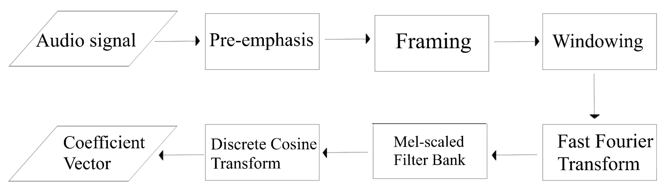
The calculation of the MFCC typically involves the following steps: pre-emphasis of the high frequency portion, segmentation of the signal into short-duration frames, multiplication of the frames with a desired window, calculation of fast Fourier transform, application of a Mel filter bank, and calculation of discrete cosine transform, as shown in Figure 1 [16]. This procedure is similar to the human auditory system’s perception, which is more sensitive to low-frequency components.

The transfer function that maps the frequency to the Mel-scale frequency can be expressed as follows [17]:

$$Mel\left(f\right)=2595lo{g}_{10}(1+\frac{f}{700})$$

(7)

Figure 2 shows the nonlinear Mel-frequency curve.

Generally, high frequency components in speech signals get attenuated during propagation and transmission. To compensate for this loss, a high pass Finite Impulse Response (FIR) filter is typically used. The rational transfer function for this filter is shown as (8)

$$y\left(n\right)=x\left(n\right)-\alpha x(n-1)$$

(8)

where $\alpha =0.9$ to $1.0$.

After pre-emphasis, the signal is divided into many short frames during the framing process by applying different windows that can reduce frequency leakage [18].

Fast Fourier Transform(FFT): discrete-time Fourier transform converts a speech signal from the time domain to its frequency domain [19]. It is shown as (9).

$$Y\left(k\right)=\sum _{j=1}^{n}x\left(j\right)W_n(j-1)(k-1)$$

(9)

where,

$$W_n=e^{(-2\pi i)/n}$$

In the Mel-frequency analysis, a bank of triangular filters is used to compute the power spectrum. Each filter is a triangle-shaped band pass filter with decreasing magnitude towards its edges. The central frequency of each filter is distributed according to the Mel-scale. After passing the signal through the filter bank, the output values are converted to a logarithmic scale to obtain the logarithmic power spectrum [20]. The logarithm formula used for this purpose is

$$L_m=log(\sum _{k=0}^{N-1}{\left|Y\left(k\right)\right|}^2{H}_m\left(k\right)),0\le m\le M$$

(10)

where N is the number of discrete Fourier transform points, and M is the MFCC order.

The last step is using discrete cosine transform (DCT) to transfer the logarithmic power spectrum from a Mel-scaled frequency domain back into its time domain [21]. Equation (11) represents the procedure.

$$C_m\left(k\right)=\sqrt{\frac{2}{N}}\sum _{n=1}^N{L}_m\left(n\right)\frac{1}{\sqrt{1+{\delta }_{k1}}}cos(\frac{\pi }{2N}(2n-1)(k-1))$$

(11)

For a signal x of length N, and with $\delta$ the Kronecker delta, k is the order of the coefficient [22].

3.4. Bark Frequency Cepstral Coefficients (BFCCs)

This technique employs the concept of Bark Frequency Cepstral Coefficients (BFCCs), which is a pitch-perception-based feature extraction process used to classify voice features [23]. The Bark-scale has a scaling factor that is modified by multiplying the initial frequency scale. The formula for converting the frequency to Bark is:

$$Bark\left(f\right)=13arctan\left(0.00076f\right)+3.5arctan({(\frac{f}{7500})}^2)$$

(12)

In BFCCs, filter banks are used in the Bark-scale, and the overall procedure is similar to that used in MFCCs, except for the filter bank transition from the Mel-scale to the Bark-scale.

4. Innovative Features

4.1. Pitch and Partials Amplitude Gradient Feature

We have proposed an innovative feature that enables the tracking of amplitude changes in the fundamental frequencies of speech signals. This algorithm calculates the first-order temporal derivatives of the fundamental frequency and its harmonics, creating a new feature.

4.1.1. Fundamental Frequency and Its Harmonics for Speech Signal

To prepare the speech signal for analysis, we first conduct pre-emphasis and framing. Next, we applied a Hamming window to reduce frequency leakage [24].

$$w\left(n\right)=0.54-0.46cos(2\pi \frac{n}{N})$$

(13)

Following the fast Fourier transform of the signal, the amplitude of the pitch and partials can be obtained by analyzing the spectrum of the signal in one frame. We selected the 10 most significant frequencies, sorted them from low to high, and generated a two-dimensional amplitude-frequency matrix, as shown in matrix (14). The matrix contains the amplitudes $a_1\cdots a_{10}$ and their corresponding frequencies $f_1\cdots f_{10}$, which are sorted from small to large.

$$\left[\begin{array}{cc}{a}_1& f_1\\ a_2& f_2\\ ⋮& ⋮\\ a_{10}& f_{10}\end{array}\right]$$

(14)

4.1.2. Derivation

During articulation, muscles supporting the articulators (e.g., the lips, tongue, and vocal cords) move, resulting in the production of speech sounds, and the amplitude of each frequency in the speech signal changes accordingly. Therefore, the pronunciation procedure can be monitored by inspecting the amplitude changes. Based on this, we propose a hypothesis that when people pronounce the same phoneme, the amplitude in each frequency has the same trend of change.

To track and quantify this trend, we reshape the amplitude-frequency matrix into a one-dimensional vector and combine all the vectors generated in different frames together. Then, we take the derivative of the amplitude to obtain the derivation matrix. As shown in matrix (15), every column (superscript) represents the elements in the same frame, and every row (subscript) represents elements in the same pitch frequency. Here, n is the number of frames, and $dt$ is the step size used in the framing process, which is relatively short in our case.

$$\begin{array}{c}\frac{d}{dt}{\left[\begin{array}{cccc}{a}_1^{\left(1\right)}& a_1^{\left(2\right)}& \cdots & a_1^{\left(n\right)}\\ a_2^{\left(1\right)}& a_2^{\left(2\right)}& \cdots & a_2^{\left(n\right)}\\ ⋮& & \ddots & ⋮\\ a_{10}^{\left(1\right)}& a_{10}^{\left(2\right)}& \cdots & a_{10}^{\left(n\right)}\end{array}\right]}_{10\times n}=\end{array}$$

(15)

$$\begin{array}{c}{\left[\begin{array}{cccc}{d}_1^{\left(1\right)\left(2\right)}& d_1^{\left(2\right)\left(3\right)}& \cdots & d_1^{(n-1)\left(n\right)}\\ d_2^{\left(1\right)\left(2\right)}& d_2^{\left(2\right)\left(3\right)}& \cdots & d_2^{(n-1)\left(n\right)}\\ ⋮& & \ddots & ⋮\\ d_{10}^{\left(1\right)\left(2\right)}& d_{10}^{\left(2\right)\left(3\right)}& \cdots & d_{10}^{(n-1)\left(n\right)}\end{array}\right]}_{10\times n-1}\end{array}$$

We start by normalizing the derivation matrix and the amplitude-frequency matrix separately. We then combine the derivation matrix with the second column of the amplitude-frequency matrix, representing the frequency, into a one-dimensional feature vector. We refer to this feature as the Pitch and Partials Amplitude Gradient Feature.

$$\begin{array}{ccccccc}[d_1^{\left(1\right)\left(2\right)}& \cdots & d_1^{(n-1)\left(n\right)}& f_1^{\left(1\right)}& \cdots & f_1^{\left(n\right)}& \cdots \\ d_{10}^{\left(1\right)\left(2\right)}& \cdots & d_{10}^{(n-1)\left(n\right)}& f_{10}^{\left(1\right)}& \cdots & f_{10}^{\left(n\right)}]\end{array}$$

(16)

4.2. Speech Wave Function Probability Amplitude Feature

4.2.1. Model Speech Signal by Using Concept of Schrödinger Equation

This section is a brief introduction to the Schrödinger equation. The Schrödinger equation is a fundamental equation in quantum mechanics that describes the time evolution of a quantum state.

The Schrödinger equation is a partial differential equation, and its solution gives the probability amplitude of finding the quantum system in a particular state at a given time. The wave function $\psi$ can be used to calculate various physical quantities, such as the probability density of finding a particle in a particular location, or the expectation value of an observable physical-like energy or momentum.

The Schrödinger equation has revolutionized our understanding of the behavior of particles at the quantum level and is essential in many areas of physics, chemistry, and engineering.

Quantum mechanics describes the properties of systems by using a wave function, $\Psi (x,t)$ and we get it by solving the Schrödinger equation [25]:

$$i\hslash \frac{\partial \Psi }{\partial t}=-\frac{{\hslash }^2}{2m}\left(\frac{{\partial }^2\Psi }{\partial x^2}\right)+V\Psi$$

(17)

Here, i is the square root of −1, and ℏ is Planck’s constant, which is the original constant h divided by 2$\pi$:

$$\hslash =\frac{h}{2\pi }=1.054573\times {10}^{-34}Js.$$

Centered on Porn’s mathematical analysis of the wave function, ${|\Psi (x,t)|}^2$ is the probability of discovering a particle x and the time t [25]. When we look at exponential activity in the time coordinate for the first time, we guess $\Psi (x,t)=e^{-i\omega t}f\left(x\right)$ and use the method of separation of variables to solve the Schrödinger equation:

$$\Psi (x,t)=\psi \left(x\right)f\left(t\right)$$

(18)

$$\frac{\partial \Psi }{\partial t}=\psi \frac{df}{dt},\frac{{\partial }^2\Psi }{\partial x^2}=\frac{d^2\psi }{d{x}^2}f$$

(19)

So, the Schrödinger equation changes the form to:

$$i\hslash \psi \frac{df}{dt}=-\frac{{\hslash }^2}{2m}\frac{d^2\psi }{d{x}^2}f+V\psi f$$

(20)

Dividing by $\psi f$:

$$i\hslash \frac{1}{f}\frac{df}{dt}=-\frac{{\hslash }^2}{2m}\frac{1}{\psi }\frac{d^2\psi }{d{x}^2}+V$$

(21)

The left side is the time function t, and the right side is the location function x. It only occurs when all sides are constant and when the divergence constant is labeled E in quantum mechanics.

$$i\hslash \psi \frac{df}{dt}=E,$$

(22)

or

$$\frac{df}{dt}=-\frac{iE}{\hslash }f$$

(23)

and

$$-\frac{{\hslash }^2}{2m}\frac{1}{\psi }\frac{d^2\psi }{d{x}^2}+V=E$$

(24)

or

$$-\frac{{\hslash }^2}{2m}\frac{d^2\psi }{d{x}^2}+V\psi =E\psi$$

(25)

The equation describing a particle with a definite energy, known as the time-independent Schrödinger equation, is more stringent than the initial Schrödinger time-dependent equation. This is because the time-independent equation culminates in two ordinary differential equations instead of one partial differential equation, with the constant E representing the particle’s total energy (kinetic plus potential) [25]. The general solution of the time-dependent Schrödinger equation, represented by Equation (23), is given by $Cexp(-iEt/\hslash )$, where C is a constant that is absorbed into $\psi$. Then, we apply

$$f\left(t\right)=e^{-iEt/\hslash }.$$

(26)

4.2.2. Infinite Square Well Model

To solve the time-dependent Schrödinger equation, we can make use of the infinite square well model. This model system in quantum mechanics consists of a particle that is confined to a one-dimensional box with infinite potential energy at the boundaries. It is used to study the behavior of a particle in a potential well with fixed boundaries, which can be an idealization of certain real-world systems, such as electrons in a solid or a gas trapped in a container.

The wave function of the particle in the infinite square well can be found analytically, and it exhibits some interesting properties, such as the quantization of energy levels and the absence of probability density outside of the box. By studying this simple model, we can gain insight into more complex quantum systems, such as atoms and molecules.

$$V\left(x\right)=\left\{\begin{array}{cc}0,\hfill & \mathrm{if}0\le x\le a,\hfill \\ \infty ,\hfill & \mathrm{otherwise}.\hfill \end{array}\right.$$

(27)

In quantum mechanics, this type of configuration is often referred to as a “particle in a box” (a 1D box) or “square”. The particle is free to move within the specified region, but has zero probability of escaping, much like a particle trapped inside a box. Therefore, the wave function $\psi \left(x\right)$ is equal to zero outside of the region.

The potential energy is infinite outside of the two boundaries that prevent particles from escaping. This is similar to an elastic ball being placed inside a square well, where it can move freely within the well but cannot escape due to the infinitely high walls of the well [25].

In fact, the particle has zero probability of being detected beyond the range of $\mathit{x}$ values that vary from 0 to $\mathit{L}$. This is because the particle would need to overcome the exponentially tall and infinitely high theoretical wall at the edge of the box. When the particle is outside of the specified range, $\psi \left(x\right)$ is equal to zero. Within the range, where $V\left(x\right)=0$, the time-independent Schrödinger Equation (25) takes the form:

$$-\frac{{\hslash }^2}{2m}\frac{d^2\psi }{d{x}^2}=E\psi$$

(28)

or

$$\frac{d^2\psi }{d{x}^2}=-k^2\psi ,\mathrm{where}k=\frac{\sqrt{2mE}}{\hslash }$$

(29)

We assume that $E>0$ because the reciprocal of $E<0$ is not physically meaningful. Thus, we can approach the problem dynamically, interpreting it as an oscillatory function that can be described using trigonometric functions. The general solution of Equation (29) is given by:

$$\psi \left(x\right)=Asin\left(kx\right)+Bcos\left(kx\right)$$

(30)

However, in the context of quantum mechanics, it is not immediately clear what this solution means physically. If the probability distribution were discontinuous, it would be highly problematic to say that there was something fundamentally wrong with the distribution. However, in this case (and in most other cases that are not pathological), it is reasonable to assume that the probability distribution is continuous. Therefore, we can proceed under the assumption that the solution is valid.

Applying the boundary conditions $\psi \left(0\right)=\psi \left(a\right)=0$, the equation can be rewritten as:

$$\psi \left(0\right)=Asin0+Bcos0=B$$

(31)

So $B=0$, and

$$\psi \left(x\right)=Asinkx.$$

(32)

Then $\psi \left(a\right)=Asinka$, this only happens when

$$ka=0,\pm \pi ,\pm 2\pi ,\pm 3\pi ,\dots$$

(33)

$$k_n=\frac{n\pi }{a},\mathrm{with}n=1,2,3,\dots$$

(34)

We can use Equation (29) to determine that $k=\frac{\sqrt{2mE}}{\hslash }$. Since we assume $E>0$, we can write the possible values of E as:

$$E_n=\frac{{\hslash }^2{k}_n^2}{2m}=\frac{n^2{\pi }^2{\hslash }^2}{2m{a}^2}$$

(35)

where n is a positive integer representing the energy level of the particle.

To ensure that the total probability of finding the particle in the range $0\le x\le a$ is 1, we must normalize the wave function $\psi$ by fixing the constant $\psi$ as follows:

$${\Psi }_n(x,t)=\sqrt{\frac{2}{a}}sin\left(\frac{n\pi }{a}x\right)e^{-i(n^2{\pi }^2\hslash /2m{a}^2)t}$$

(36)

4.3. Speech Wave Function-Based Probability Amplitude Feature

During the process of speech production, the vibrations generated by the vocal cords pass through the vocal tract to create specific sounds. Although every individual is unique, the changes over time and space of these vibrations should be similar when making the same sound. Therefore, the shape and movement of the interaction among all involved biological structures generate an acoustic waveform. This means that all the information is embedded in the time-domain and frequency-domain characteristics with different probabilities. However, the commonly used features for speech signals, such as Mel-frequency cepstral coefficients, do not explicitly capture the probability information of the signal.

To address this issue, we introduce the concept of a frame probability feature in speech signal processing. Frames with a high probability receive a greater coefficient, resulting in a higher degree of discrimination in the feature vector.

To improve the Mel-frequency cepstrum coefficient, we apply the infinite square well model in feature extraction. We can use the concept of probability from the wave function. Just as the infinite square well restricts the particle, the speed of sound limits the audio to a particular range if we determine the length of time. The stationary states Equation (36) is used to calculate the probability in each frame. To calculate this equation, we need to know every frame’s time, position in space, and energy. 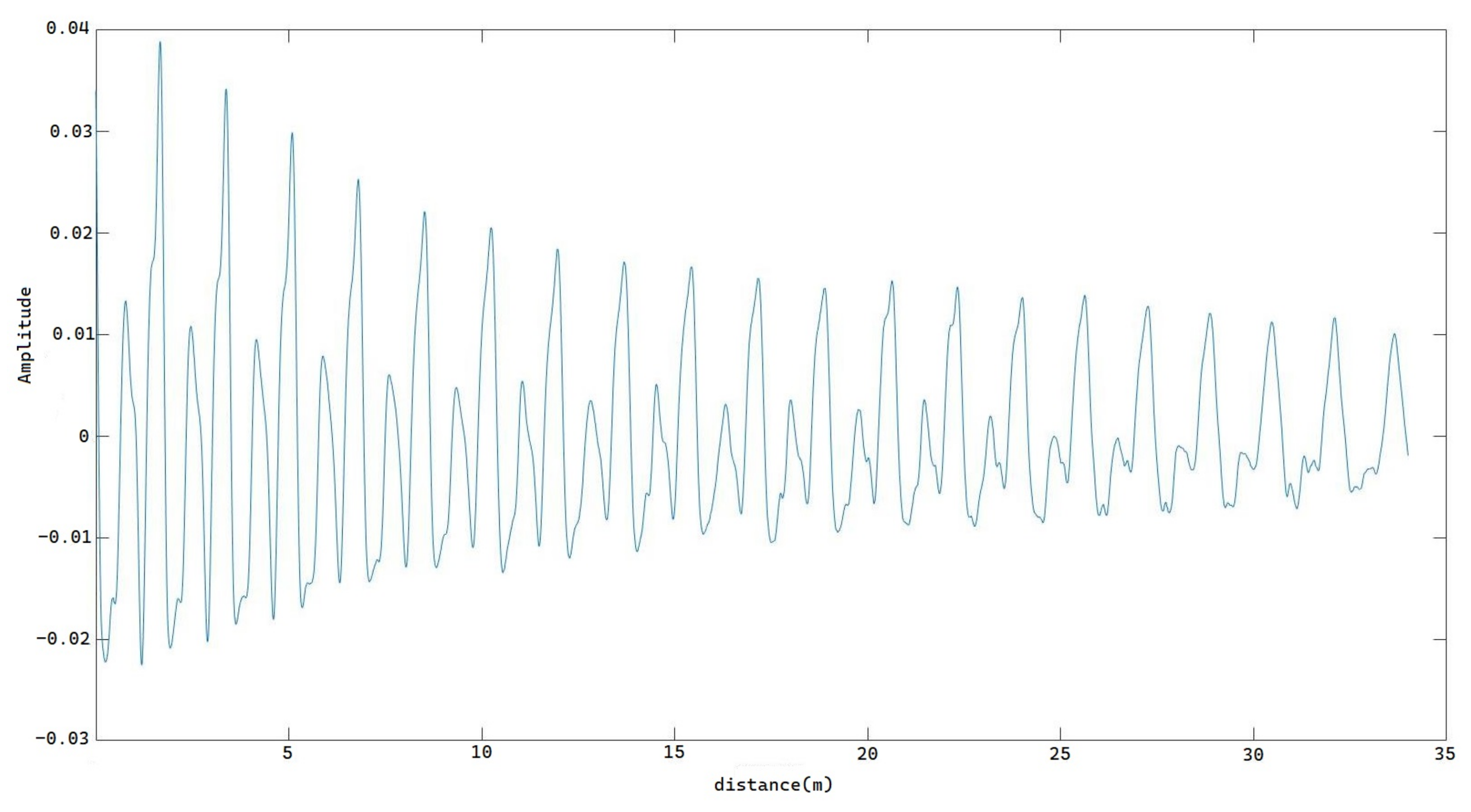Figure 3 shows an audio sample of the phoneme /r/ in the time domain, which we recorded near the speaker’s mouth. The characteristics of the audio signal contain all the information embedded in the time domain and frequency domain with different probabilities.

We also need to consider how the audio is distributed in space. Assuming the speed of sound is 340 m/s, we can calculate that the sound wave can travel a distance of 34 m during the 0.1-second duration. Therefore, the sound wave originating from the speaker’s mouth will be located 34 m away at the beginning of the recording. Similarly, the sound wave at the end of the recording will be located at the microphone’s position, which we can assume is at position zero. Figure 4 shows the audio distribution of the same sample in space.

This new feature can be interpreted as a probability-based feature, which is calculated based on the time, position, and energy of each sampling point in a complex manner and provides a way to incorporate the probability information of each frame into the Mel-frequency cepstrum coefficient (MFCC) feature. The procedure consists of pre-emphasis and framing, calculating the wave function $\Psi (x,t)$, and obtaining the probability ${|\Psi (x,t)|}^2$. We then add up all probabilities of samples within one frame to obtain the total probability of that frame. We continue with the MFCC procedure, which includes windowing, applying Fast Fourier Transform, applying a Mel-scaled filter bank, and applying Discrete Cosine Transform to obtain the original MFCC features of that frame. Finally, we multiply the MFCC features by the probability of that frame to obtain the new feature.

5. Classification Methods

In this paper, we use a hypothesis $H=1$ to represent the classification result of standard English pronunciation of /r/, and use hypothesis $H=0$ to represent the classification result of a non-standard English /r/. We use $L=1$ to represent speech labeled as standard English speakers, and $L=0$ to represent speech labeled as non-standard English speakers.

5.1. K-Nearest Neighbor (KNN)

One of the most basic and straightforward classification techniques is K-nearest neighbor classification. The KNN algorithm works based on the principle that if the majority of the most similar samples in the feature space (i.e., the sample’s closest neighbor in the feature space) belong to the same group, then the sample does as well [26]. The Euclidean distance between a reference sample and the training samples is typically used as the basis for the K-nearest neighbor classifier.

Data in the training set L, are classified by this algorithm into several separate categories, $C_1,\dots ,C_M$, with M as the number of categories. In the jth category, there are samples $\{(x_1^{\left(j\right)}),\cdots ,(x_n^{\left(j\right)})\}$, where n is the number of samples and features are N dimension vectors. The expectation of each category will be

$${\mu }^{\left(j\right)}=\frac{1}{n}\sum _{i=1}^n{x}_i^{\left(j\right)}$$

(37)

Then, we can calculate the distance of each sample in the testing dataset, $X_1,\cdots ,X_n$, to each category expectation, ${\mu }^{\left(j\right)}$, using Equation (38).

$$d_j=\sqrt{{(X_i-{\mu }^{\left(j\right)})}^2}$$

(38)

Because this is a binary classification, the value of the threshold affects the classification rate. We can investigate the performance of the classifier by changing the threshold and using a receiver operating characteristic curve. The classification logic for a given threshold $V_i$ is shown in (39).

$$\begin{array}{c}H=\left\{\begin{array}{cc}1,\hfill & \mathrm{if}\frac{d_1}{d_2}\le V_i\hfill \\ 0,\hfill & \mathrm{if}\frac{d_1}{d_2}>V_i\hfill \end{array}\right.\end{array}$$

(39)

5.2. Gaussian Multivariate Model (GMM)

A Gaussian Mixture Model (GMM) is a statistical model that assumes that the probability distribution of the observed data points comes from a mixture of several Gaussian distributions, each with its own mean and covariance. The model is trained to learn the parameters of these Gaussian distributions and the probabilities of each data point belonging to each of the Gaussian distributions. Once trained, the GMM can be used for a variety of tasks such as clustering, density estimation, and classification (40).

The mean and the covariance matrix of the GMM can be obtained from the training dataset [27].

$$\mu =\frac{1}{n}\sum _{i=1}^n{x}_i$$

(40)

$$\mathbf{\Sigma }=E\left[(x-\mu ){(x-\mu )}^T\right]$$

(41)

In order to calculate fast, we extract the diagonal elements of $\mathbf{\Sigma }$ and generate a diagonal matrix to replace the original covariance matrix. To expedite calculations, we can extract the diagonal elements of the covariance matrix, denoted by $\mathbf{D}$, and create a diagonal matrix by placing these elements along the main diagonal. This diagonal matrix can then be used to replace the original covariance matrix in computations, leading to faster processing times.

$$\mathbf{D}=\left[\begin{array}{cccc}{\sigma }_1^2& & & \\ & {\sigma }_2^2& & \\ & & \ddots & \\ & & & {\sigma }_N^2\end{array}\right]$$

(42)

The probability density function (PDF) of the Gaussian Multivariate Model is shown by the following Equation (43):

$$p_i(x;\mu ,\Sigma )=\frac{1}{{\left(2\pi \right)}^{\frac{N}{2}}{\left|\mathbf{\Sigma }\right|}^{\frac{1}{2}}}{e}^{(-\frac{1}{2}{(X_i-\mu )}^T{\mathbf{\Sigma }}^{-1}(X_i-\mu ))}$$

(43)

After calculating the PDF of a testing sample using Gaussian Mixture Models (GMMs), the testing sample can be classified as belonging to the Gaussian component with the highest posterior probability. In other words, for each Gaussian component in the GMM, we can compute the posterior probability that the testing sample belongs to that component given its observed features. The testing sample is then classified as belonging to the component with the highest posterior probability.

5.3. Artificial Neural Network

An Artificial Neural Network (ANN) is a popular classifier used in various fields such as image recognition, natural language processing, speech recognition, and many others. An ANN is a type of machine learning model that is designed to simulate the behavior of the human brain’s neural networks.

The basic structure of an ANN consists of an input layer, one or more hidden layers, and an output layer. The nodes in the input layer receive the input data, which are then processed by the nodes in the hidden layers to extract important features. The output layer then produces the final output based on the learned features.

The learning process of an ANN involves training the network on a labeled dataset, where the network adjusts its weights and biases to minimize the difference between the predicted output and the true output. This process is typically performed using an optimization algorithm such as backpropagation.

One of the strengths of an ANN is its ability to learn complex patterns and relationships in data, making it suitable for a wide range of classification tasks. Additionally, an ANN can handle noisy or incomplete data, and can generalize unseen data well, making it a powerful tool for machine learning. The activation function in an ANN is (44),

$$S\left(x\right)=\frac{1}{1+e^{-x}}$$

(44)

The ability to learn from training data and generalize results using active function is one of the main characteristics of an artificial neural network; it stores the knowledge gained during the training process in the synaptic weights of the neurons [28].

The synaptic weight of a connection between two nodes is a value that represents the connection between the two nodes. The way nodes are connected, connection weight values, and the activation function all affect the output of a neural network model.

For an ANN, the input layer is the input signal, and the hidden layer and output layer are assembled by cells [29].

For m samples {$x^{\left(1\right)}{y}^{\left(1\right)}\cdots x^{\left(m\right)}{y}^{\left(m\right)}$}, the cost function of applying a neural network is Equation (45).

$$\begin{array}{cc}\hfill J\left(\theta \right)=& -\frac{1}{m}[\sum _{i=1}^m\sum _{k=1}^k{y}_k^{\left(i\right)}{log(h_{\theta }(x^{\left(i\right)}))}_k\hfill \\ \hfill & +(1-y_k^{\left(i\right)}){log(1-h_{\theta }(x^{\left(i\right)}))}_k\left)\right]\hfill \\ \hfill & +\frac{\lambda }{2m}\sum _{l=1}^{L-1}\sum _{i=1}^{S_L}\sum _{j=1}^{S_L+1}{({\theta }_{ji}^{\left(l\right)})}^2\hfill \end{array}$$

(45)

where the input data x are represented as features, the output data y represent the label of the training sample, and the weight matrix between the network’s cells is denoted by $\theta$. To prevent overfitting, a regularization parameter $\lambda$ is introduced. The network typically consists of L layers, with $S_l$ representing the number of units in layer l. The objective of the ANN is to find the weight matrix $\theta$ that minimizes the cost function.

The backpropagation algorithm is a supervised learning algorithm used to train Artificial Neural Networks (ANNs) to make accurate predictions for a given input. The name “backpropagation” refers to the fact that the algorithm works by propagating the error from the output layer back through the network, adjusting the weights of the connections between neurons as it goes. During the training process, the backpropagation algorithm calculates the error between the network’s output and the desired output, and then adjusts the weights of the connections between neurons in the network to minimize this error. This is typically performed using a gradient descent optimization algorithm, which calculates the gradients of the error with respect to each weight in the network, and then adjusts the weights in the direction of the steepest descent.

6. Experiment and Result

6.1. Data Collection and Labeling

In this project, we recruited 31 human subjects, including 19 native English speakers and 12 nonnative English speakers. All participants were asked to read a file containing 40 words with the phoneme ‘r’ sound in word initial position followed by a variety of vowels. Their speech signals were recorded using a SONY PCM-D50 two-channel linear digital recorder. The sample of a part of the file was shown in the

Table 1. Sample of word list.

r and Adjacent Vowel	Words
/ru/	rude
/ru/	room
/ru/	ruse
/ru/	root
/ri/	reach
/ri/	reef
/ri/	reason
/ri/	read

. The recordings were conducted either in the communication lab at the School of Allied Health and Communicative Disorders, or at the Digital Signal Processing lab, Northern Illinois University. To ensure a quiet recording environment, we aimed to maintain an average ambient noise level of less than 45 dB during the recording procedure. The sampling rate was set at 48 kHz, and a data file with two channels was obtained for each participant.

The duration of the phoneme /r/ in a word is approximately 0.085 s, so we extracted the first 0.1 s of the speech segment from each word as a data sample.

In this research, which is a binary classification problem, we defined two categories for each data instance: ’correct 1’ and ’incorrect 0’. The initial labeling process for the data instances was conducted by a professional speech-language pathologist, who determined whether each instance represented the correct or incorrect pronunciation of the phoneme /r/. Then, we divided the labeled data into training and testing sets. The training set is used to train the machine learning model, while the testing set is used to evaluate the model’s performance.

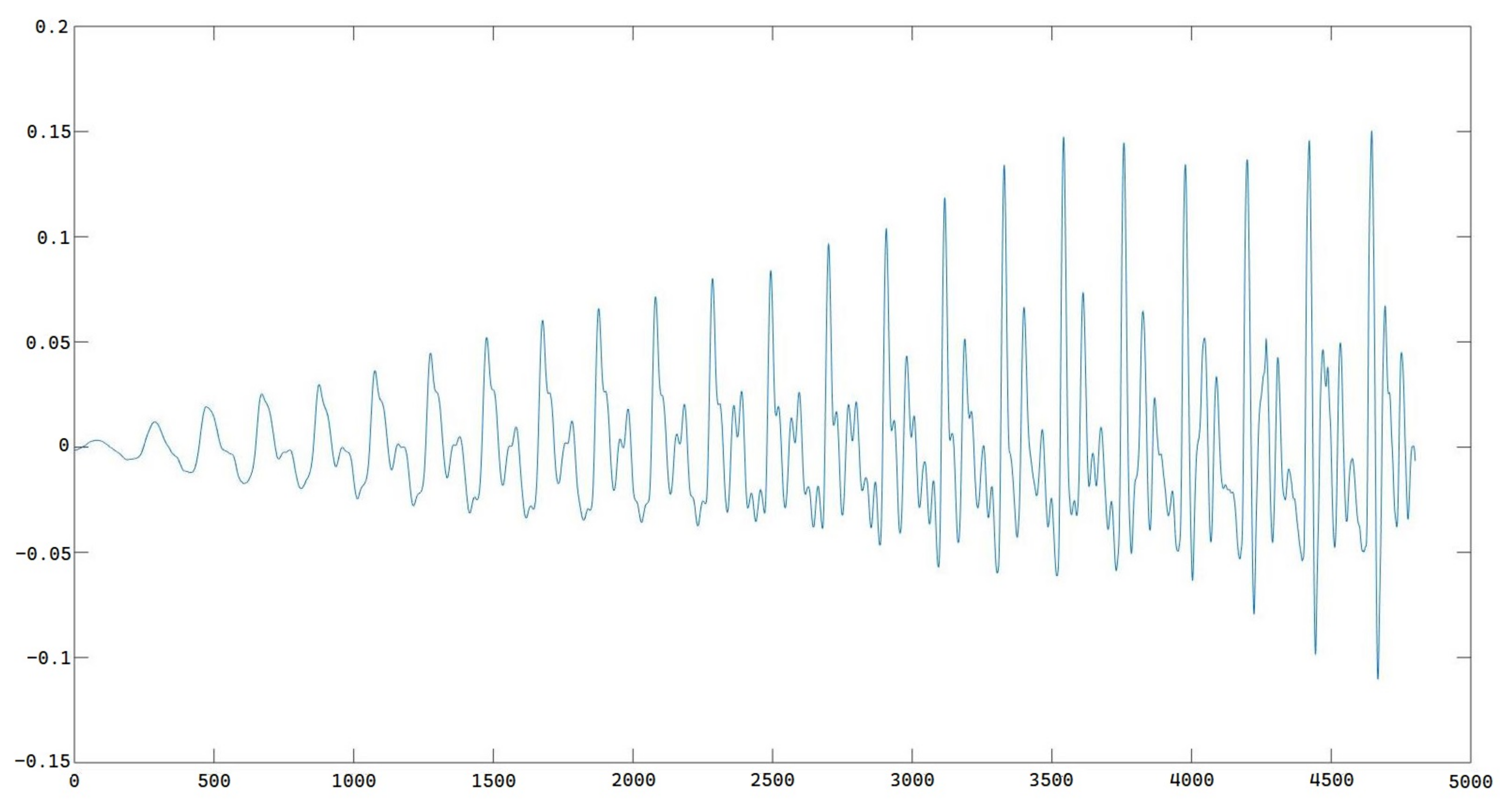
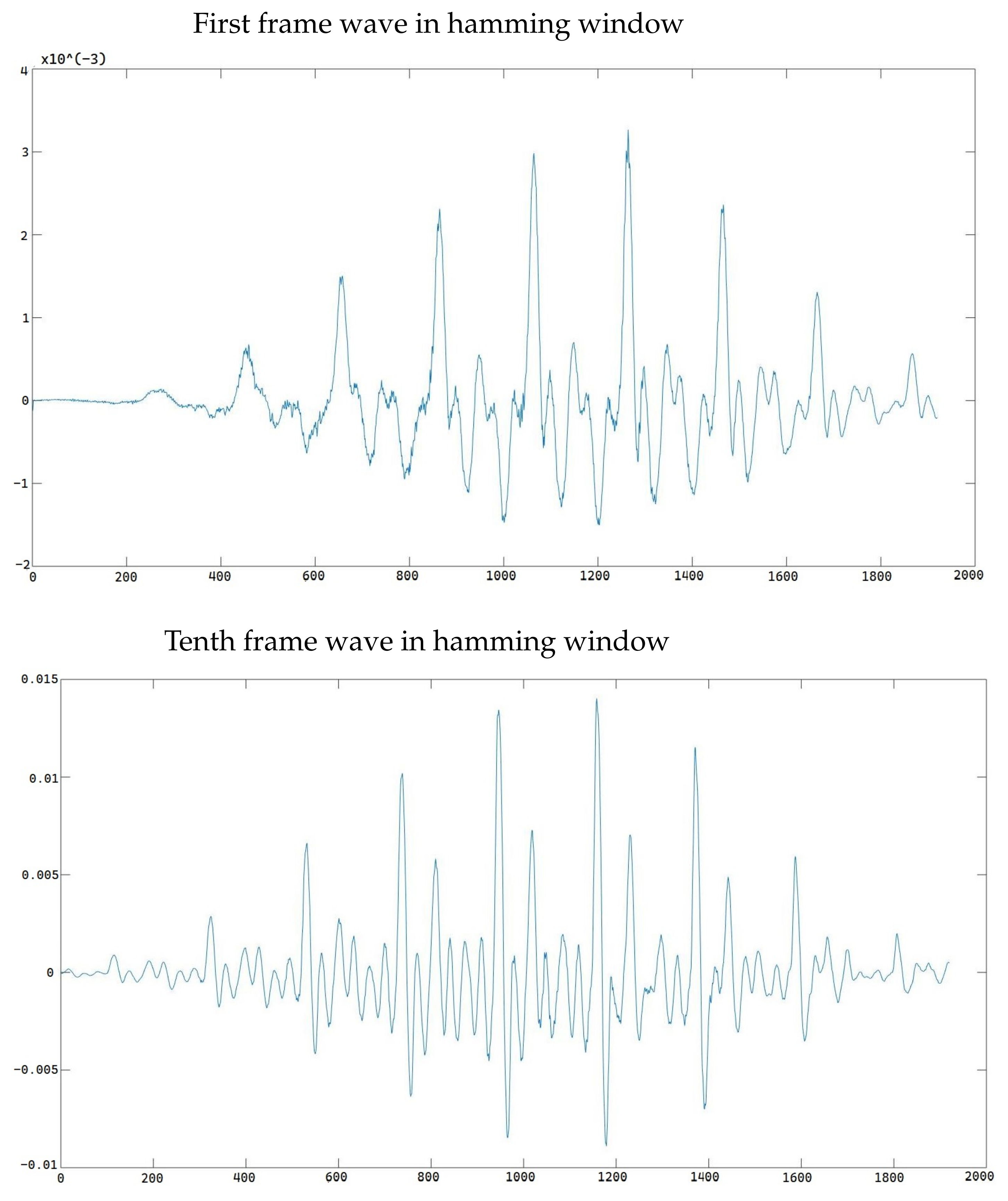
The first 0.1 s part from an original waveform from a native English speaker is shown in Figure 5.

6.2. Pre-Processing

The pre-emphasizing high pass FIR filter we used is $y\left(n\right)=x\left(n\right)-0.98x(n-1)$. The audio wave after passing the filter is shown as Figure 6.

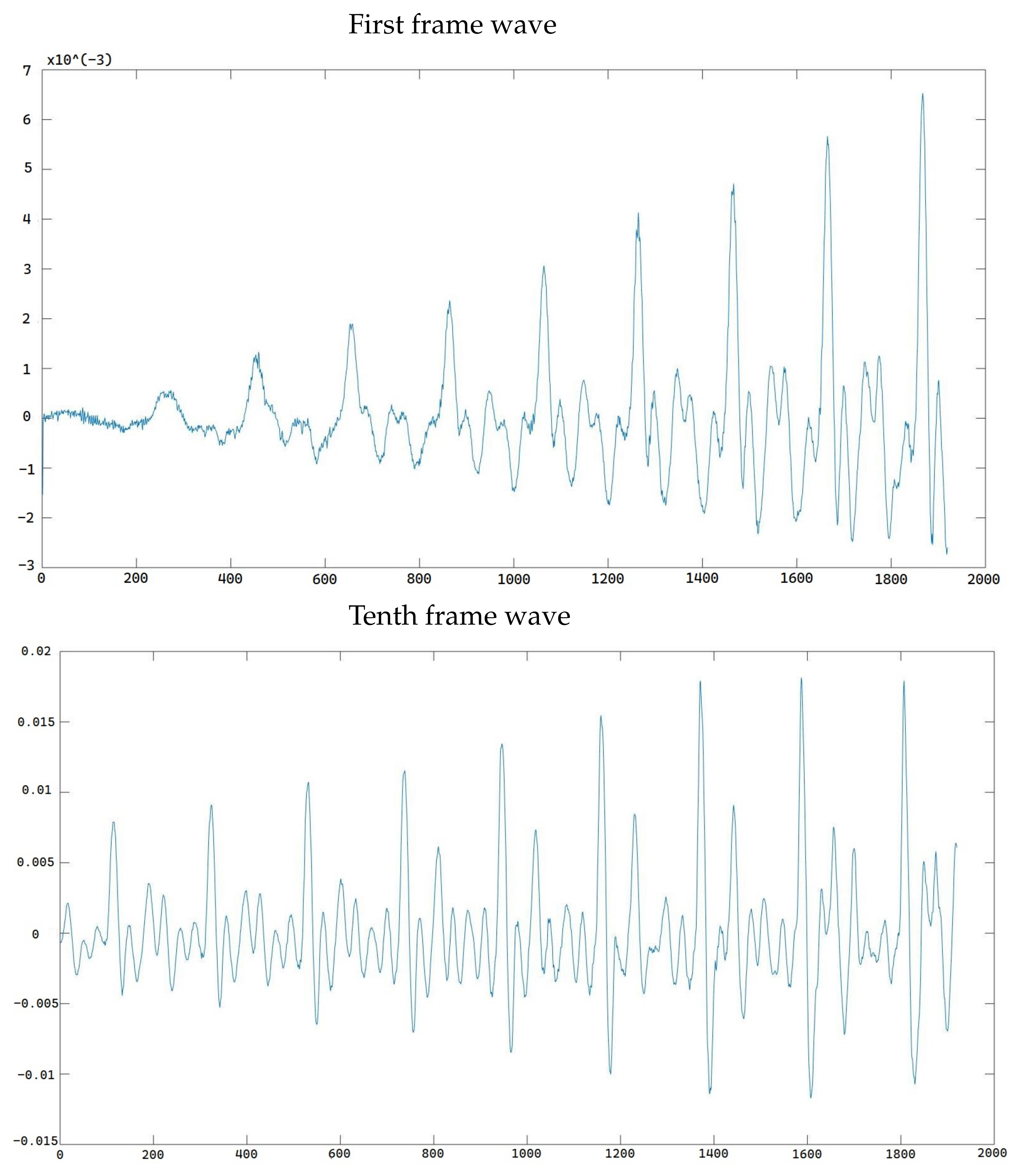
We chose the frame length as 40 ms with an overlap rate of 6.3% and we obtained 10 frames from each data sample for analysis. Figure 7 shows the difference in signal between the first frame and tenth frame.

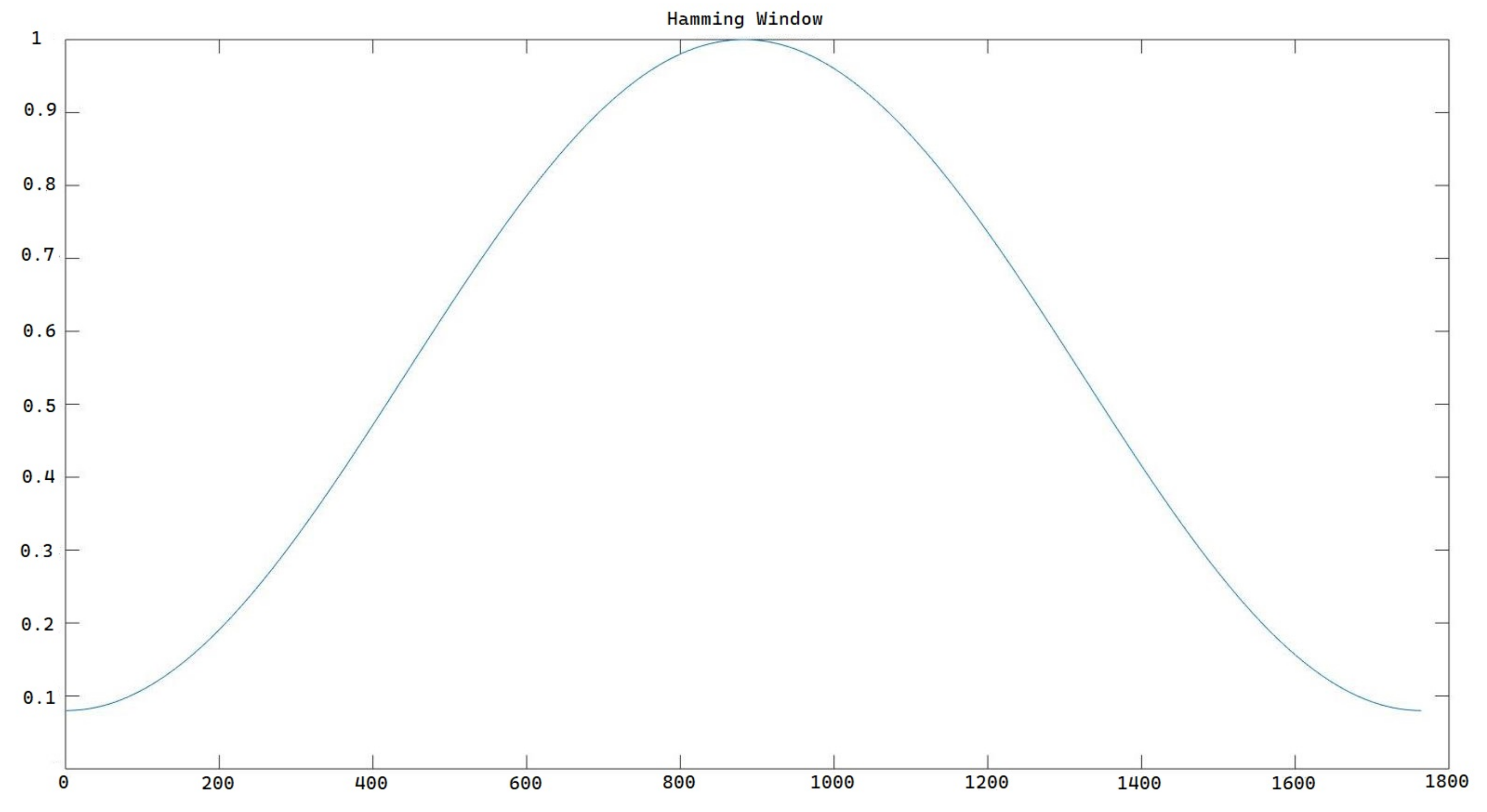
Then, we used a hamming window, shown in Figure 8, to multiply each frame, as shown in Figure 9.

6.3. Feature Extraction

6.3.1. MFCC Features

We extract the MFCC feature, which is one of the the most popular features used for speech recognition, as a comparison baseline. The frame length is 0.025 s, the frame step is 0.01 s and the overlap rate is 60%. For each /r/ production, we get a total of 8 frames and we select 13 coefficients as features in 1 frame. Finally, the feature vector is a vector of 104 elements.

6.3.2. Pitch and Partials Amplitude Gradient Feature

We applied the fast Fourier transform to each frame of the speech signal, and then we searched for the peak amplitude in the frequency domain. As shown in Figure 10, when we compare the FFT figures obtained from the 1st and 10th frames, we can see that the pitch frequency does not change significantly, but the amplitude in each frequency changes dramatically.

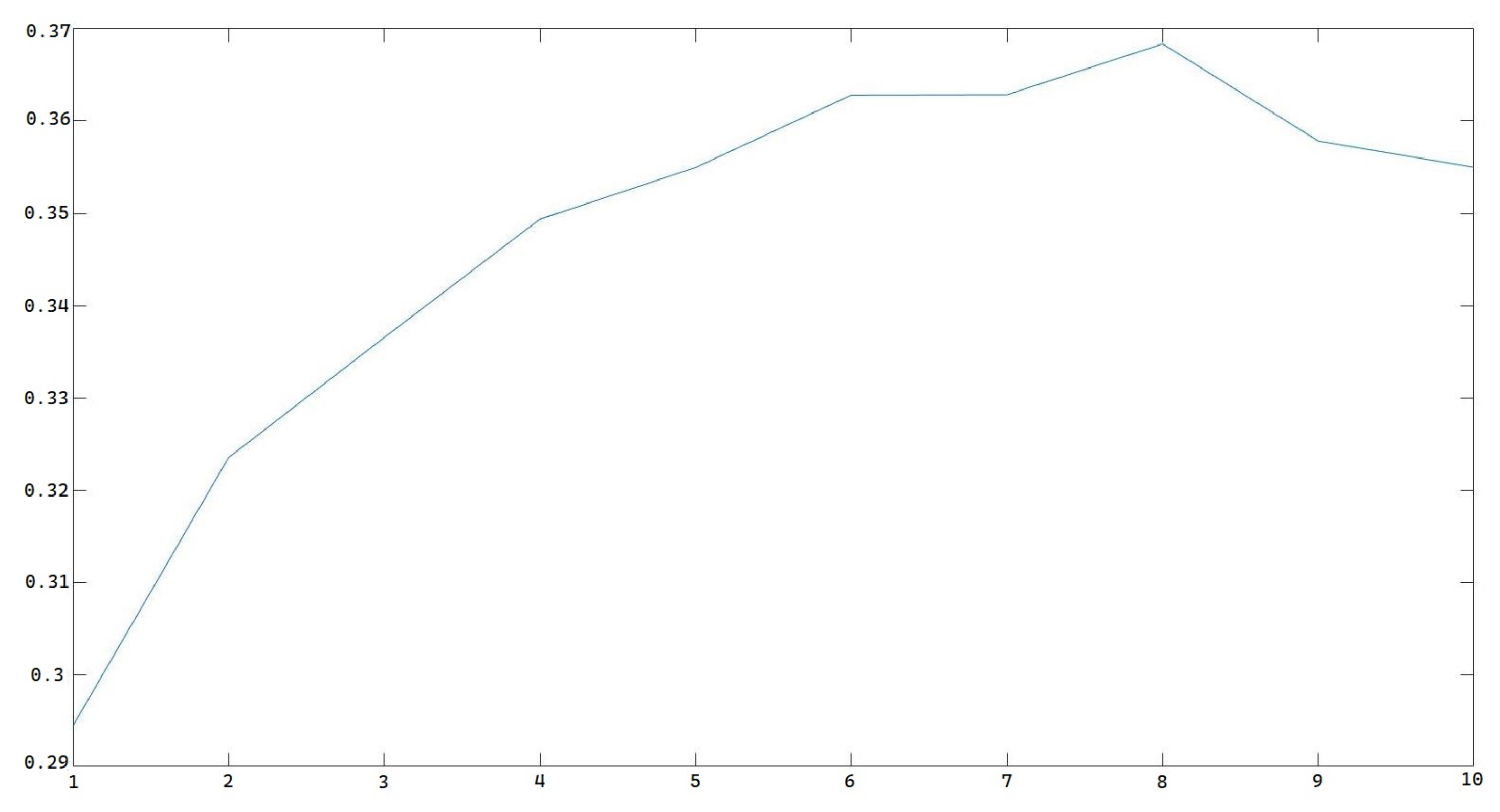
We then obtained the amplitude-frequency matrix shown in Equation (14), which is a $10\times 2$ matrix. For a particular frequency, we can analyze the trend of amplitude changes across different frames. Figure 11 shows the amplitude changing trend for the pitch frequency of 225 Hz.

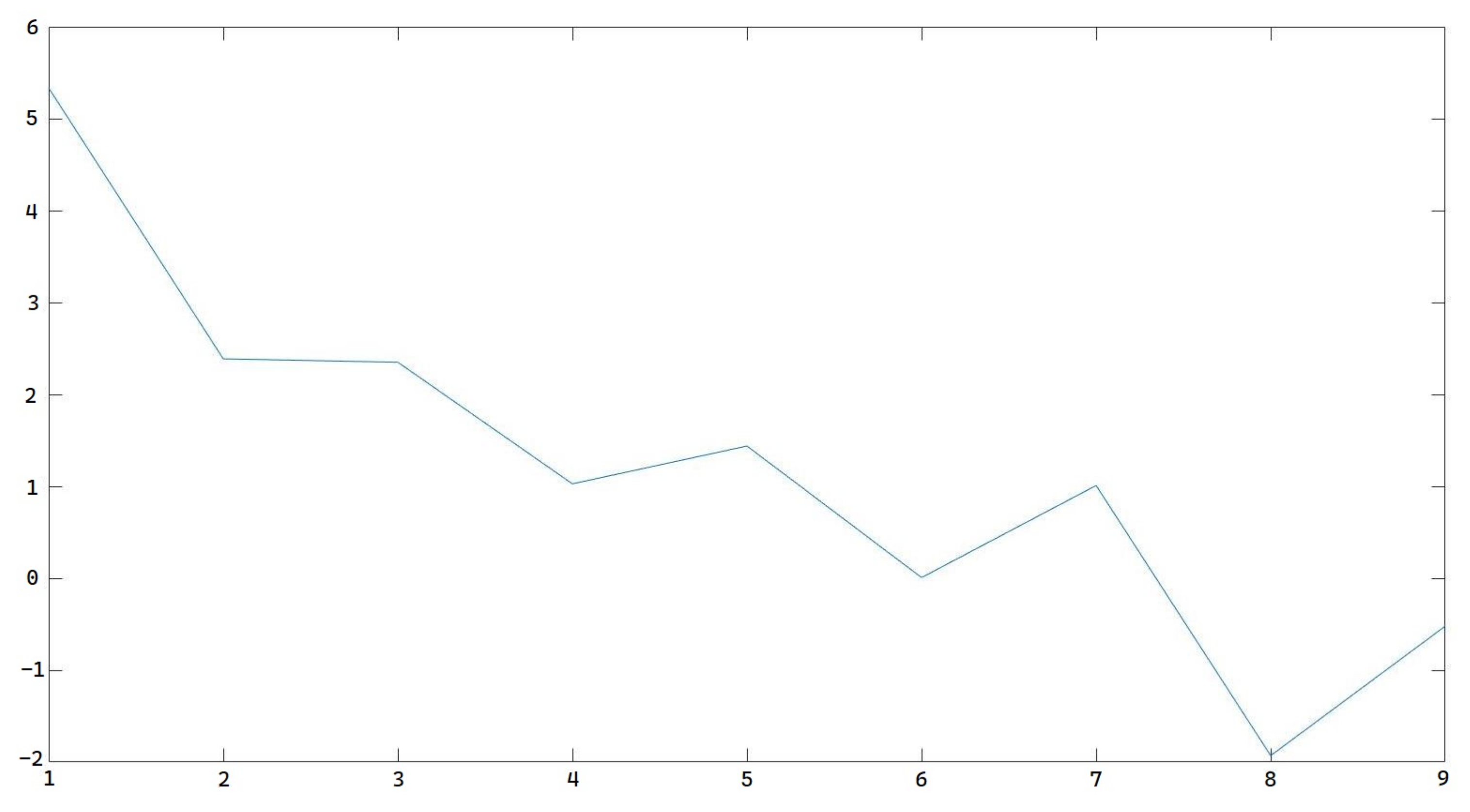
Next we calculated the derivation of the amplitude part from each frame with the same pitch frequency as matrix (15). In this case, we have 10 frames, so the derivation matrix will be a $10\times 9$ matrix. The derivation matrix quantifies the amplitude changes with the time changes. Figure 12 shows the derivation representing the amplitude changing trend in the 225 Hz pitch frequency.

Finally we calculated the derivation matrix and obtained the pitch and partials amplitude gradient features which include 190 elements.

6.3.3. Speech Wave Function Probability Features

In this experiment, we have 2480 audio samples of the phonetic /r/ pronunciation, each with a duration of 0.1 s. These samples include 1520 labeled ‘1’ and 960 labeled ‘0’. The recorder’s sampling rate is 48,000 Hz. The rational transfer function index $\alpha$ is 0.93. We use a frame length of 0.025 s and a frame step of 0.01 s, resulting in an overlap rate of 60% and the generation of eight frames. Each frame contains 1200 sampling points, with each sampling point having a value of amplitude, whose square value represents the energy, time, and corresponding spatial location. We can then use the stationary state wave function (37) for analysis.

$${\Psi }_n(x,t)=\sqrt{\frac{2}{a}}sin\left(\frac{n\pi }{a}x\right)e^{-i(n^2{\pi }^2\hslash /2m{a}^2)t}$$

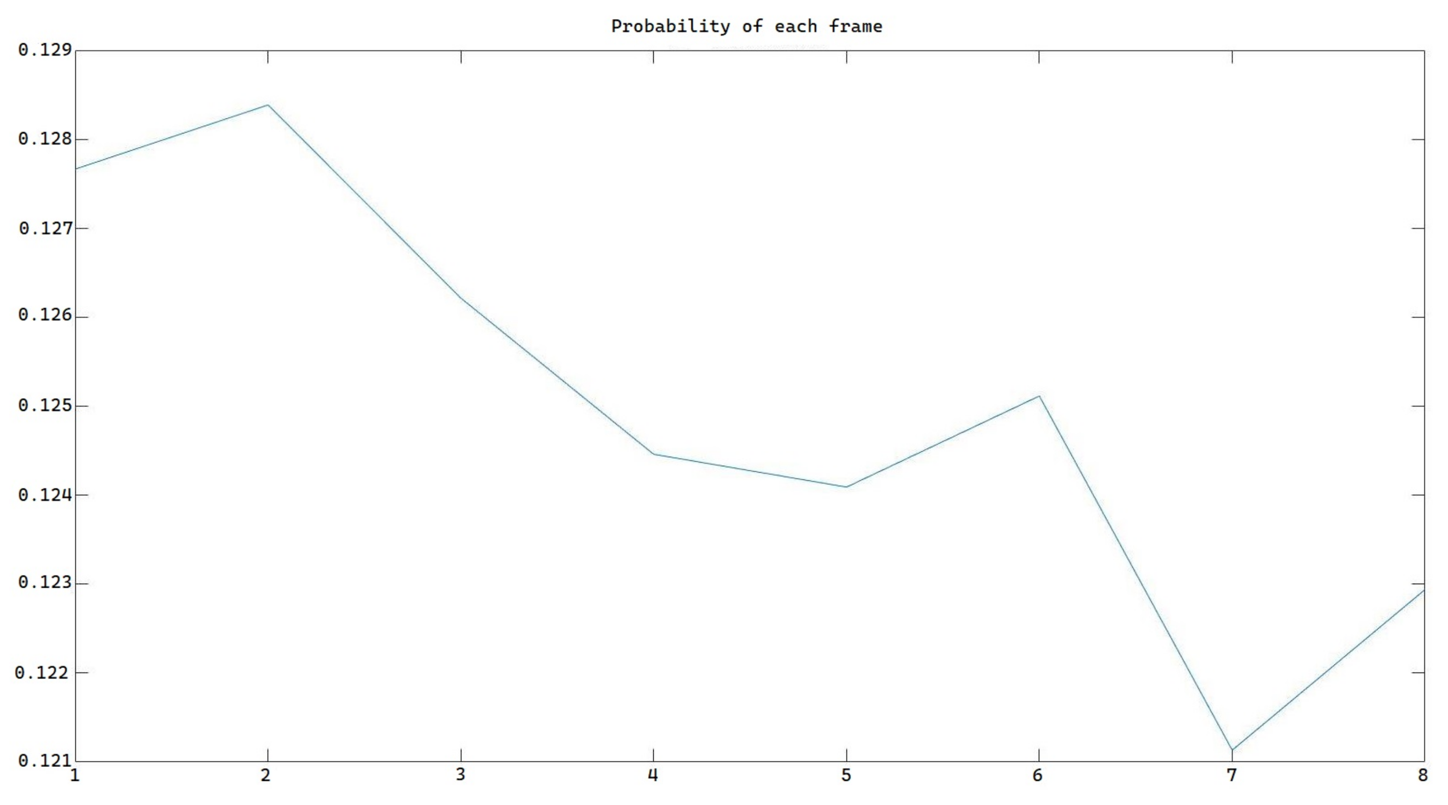
In this experiment, x represents the sampling point position in the spatial domain, while t represents time. The length of the total 0.1 s signal, denoted as a, is 34 m. We can calculate n, where $E_n$ is the square value of amplitude. The constant m is assumed to be 1 in order to reduce computational complexity. Then, we can calculate the total probability of this frame and continue with the calculation of the MFCC. A triangle window is applied afterwards. We then perform FFT and pass the resulting signal through a Mel-scaled filter bank, which is a 13-order filter bank, to obtain 13 coefficients from 1 frame. After applying Discrete Cosine Transform, we can obtain the original MFCC, which we then multiply by the probability. The probability of each frame from one standard English speaker’s pronunciation is shown in Figure 13.

The new feature is a $8\times 13$ matrix that represent the message of one production. Reshape the matrix to a vector of 104 elements.

6.4. Classification Results

In the classification part, the first algorithm used is KNN. We randomly select an audio feature for a correct and an incorrect pronunciation as the reference. Using Equation (37), we calculate the Euclidean distance for both reference features in the feature space, called ${\mu }_1$ and ${\mu }_2$. Then, we use all other data samples as the testing sample and calculate the distances ($d_1$ and $d_2$). To optimize the classification performance, we modify the original KNN algorithm by using the classification logic for a given threshold $V_i$:

$$\begin{array}{c}H=\left\{\begin{array}{cc}1,\hfill & \mathrm{if}\frac{d_1}{d_2}\le V_i\hfill \\ 0,\hfill & \mathrm{if}\frac{d_1}{d_2}>V_i\hfill \end{array}\right.\end{array}$$

(46)

the second classification algorithm is the Gaussian model. We select four native English speakers’ feature samples to calculate the expectation ( $\mu$ ) by using Equation (40) and then Equation (41) to get the covariance matrix $\mathbf{\Sigma }$ and then its diagonal matrix $\mathbf{D}$. To scale the output value we only calculate the $p=e^{(-\frac{1}{2}{(X_i-\mu )}^T{\Sigma }^{-1}(X_i-\mu ))}$ part of Equation (43). The classification logic for a given threshold $V_i$ is shown as Equation (47).

$$\begin{array}{c}H=\left\{\begin{array}{cc}1,\hfill & \mathrm{if}p>V_i\hfill \\ 0,\hfill & \mathrm{if}p\le V_i\hfill \end{array}\right.\end{array}$$

(47)

The last classifier used was an ANN, where features obtained from the previous subsection were fed into the input layer of the Artificial Neural Network. We then constructed one hidden layer with six cells and one bias cell and one output layer with two output nodes.

The comparison of the performance among different features and methods can be found in the

Table 2. Classification results for different features and methods.

	KNN CR (%)	KNN Threshold	GMM CR (%)	GMM Threshold	ANN CR (%)
MFCC	82.72	0.9053	81.77	0.4484	87.217
PPAG	79.15	0.6156	82.38	0.2148	96.97
SWPA	84.72	1.1196	80.77	0.4562	93.911

.

We obtained the maximum recognition rate for KNN and GMM classifiers by using a specific threshold value. For the ANN, we evaluated the recognition rate for all three types of features. Our results showed that the proposed speech wave function probability features achieved the highest classification rate when using the KNN classifier. For the GMM classifier, the pitch and partials amplitude features outperformed the other two features. Finally, for the ANN model, the pitch and partials amplitude features provided the highest classification rate.

7. Conclusions

In this study, we aimed to evaluate the feasibility of using a knowledge-based intelligence program to differentiate pronunciation, specifically focusing on one of the most challenging aspects of pronunciation remediation—the rhotic /r/. Our approach involved using signal analysis and classification methods. We detected speech signals containing /r/ by implementing short-time processing, extracting relevant features, and utilizing classifiers for pronunciation diagnosis. Our experiment demonstrated that the proposed knowledge-based intelligence program is a promising solution to this problem. Without the loss of generality, this approach can be extended to other rhotics.

While algorithms commonly used for speech recognition have been extensively researched, they may not be suitable for differentiating correct and incorrect rhotic pronunciation based on detailed acoustic features. Therefore, we proposed two innovative features to address this issue.

The first proposed feature focused on dynamic changes in the fundamental frequency and its harmonics, called a pitch and particle gradient feature. To capture subtle differences among correct and various incorrect pronunciations, we borrowed the concept of Schrodinger’s equation from quantum physics and developed a wave function-based probability feature from speech signals. We collected data from 31 human participants and found that these two features performed well in our experiments.

The pitch and particle gradient feature outperformed the commonly used Mel-frequency cepstral coefficients (MFCCs) feature when the Gaussian Mixture Model (GMM) and Artificial Neural Network (ANN) classifiers were employed. In addition, the wave function-based amplitude probability feature achieved the best performance when using the ANN classifier.

In future work, we plan to explore the potential of our proposed features and classifiers in other aspects of speech recognition and pronunciation assessment. Additionally, we intend to investigate the generalization of our model to larger datasets and diverse populations.

Finally, we aim to investigate the use of additional signal processing techniques and advanced machine learning models such as deep learning to further improve the performance of our proposed features and classifiers.

References

- Thompson, I. Foreign accents revisited: The English pronunciation of Russian immigrants. Lang. Learn. 1991, 41, 177–204. [Google Scholar] [CrossRef]
- Derwing, T.M.; Thomson, R.I.; Munro, M.J. English pronunciation and fluency development in Mandarin and Slavic speakers. System 2006, 34, 183–193. [Google Scholar] [CrossRef]
- Murphy, J.M. Intelligible, comprehensible, non-native models in ESL/EFL pronunciation teaching. System 2014, 42, 258–269. [Google Scholar] [CrossRef]
- Pronounce r Sound Pronuncian: American English Pronunciation. Pronuncian: American English Pronunciation. 2020. Available online: https://pronuncian.com/pronounce-r-sound (accessed on 16 March 2020).
- Wren, Y.; Pagnamenta, E.; Peters, T.J.; Emond, A.; Northstone, K.; Miller, L.L.; Roulstone, S. Educational Outcomes Associated with Persistent Speech Disorder. Int. J. Lang. Commun. Disord. 2021, 56, 299–312. [Google Scholar] [CrossRef] [PubMed]
- Hitchcock, E.R.; Harel, D.; Byun, T.M. Social, emotional, and academic impact of residual speech errors in school-aged children: A survey study. Semin. Speech Lang. 2015, 36, 283–294. [Google Scholar] [CrossRef] [PubMed]
- Silverman, F.H.; Paulus, P.G. Peer reactions to teen- agers who substitute /w/ for /r/. Lang. Speech Hear. Serv. Sch. 1989, 20, 219–221. [Google Scholar] [CrossRef]
- May-Mederake, B. Early intervention and assessment of speech and language development in young children with cochlear implants. Int. J. Pediatr. Otorhinolaryngol. 2012, 76, 939–946. [Google Scholar] [CrossRef] [PubMed]
- Shriberg, L.D.; Tomblin, J.B.; McSweeney, J.L. Prevalence of Speech Delay in 6-Year-Old Children and Comorbidity with Language Impairment. J. Speech Lang. Hear. Res. 1999, 42, 1461–1481. [Google Scholar] [CrossRef] [PubMed]
- Bleile, K.M. Speech Evaluation. In Speech Sound Disorders: For Class and Clinic; Plural Publishing: San Diego, CA, USA, 2020; pp. 149–164. [Google Scholar]
- Owens, F.J. Signal Processing of Speech; Macmillan Press Ltd.: London, UK, 1993. [Google Scholar]
- Kondoz, A.M. Digital Speech; John Wiley and Sons Ltd.: West Sussex, UK, 2004. [Google Scholar]
- Deng, L. Speech Processing: A Dynamic and Optimization-Oriented Approach; O’Shaughnessy, D., Ed.; Marcel Dekker: New York, NY, USA, 2003; pp. 41–48. [Google Scholar]
- Al-Sarayreh, K.T.; Al-Qutaish, R.E.; Al-Kasasbeh, B.M. Using the Sound Recognition Techniques to Reduce the Electricity Consumptions in Highways. J. Am. Sci. 2009, 5, 1–12. [Google Scholar]
- Yuan, Y.J.; Zhao, P.H.; Zhou, Q. Research of speaker recognition based on combination of LPCC and MFCC. In Proceedings of the 2010 IEEE International Conference on Intelligent Computing and Intelligent Systems, Xiamen, China, 29–31 October 2010; Volume 3, pp. 765–767. [Google Scholar]
- Rabiner, L.; Juang, B.-H. Fundamentals of Speech Recognition; Prentice-Hall: Englewood Cliffs, NJ, USA, 1993. [Google Scholar]
- Young, S.; Odell, J.; Ollason, D.; Valtchev, V.; Woodland, P. The HTK Book; Cambridge University: Cambridge, UK, 1997; Version 2.1, Chapter 5.4. [Google Scholar]
- Weisstein, E.W. Leakage. From MathWorld-A Wolfram Web Resource. Available online: http://mathworld.wolfram.com/Leakage.html (accessed on 11 March 2020).
- Mathworks.com. Fast Fourier Transform—MATLAB FFT. 2020. Available online: https://www.mathworks.com/help/matlab/ref/fft.html (accessed on 11 March 2020).
- Nakagawa, S.; Wang, L.; Ohtsuka, S. Speaker Identification and Verification by Combining MFCC and Phase Information. IEEE Trans. Audio Speech Lang. Process. 2012, 20, 1085–1095. [Google Scholar] [CrossRef]
- Gaurav, G.; Deiv, D.S.; Sharma, G.K.; Bhattacharya, M. Development of Application Specific Continuous Speech Recognition System in Hindi. J. Signal Inf. Process. 2012, 3, 394–401. [Google Scholar] [CrossRef]
- Mathwork.com. Discrete Cosine Transform—MATLAB DCT. 2020. Available online: http://www.mathworks.com/help/signal/ref/dct.html?s_tid=srchtitle (accessed on 12 August 2020).
- Sumithra, M.G.; Devika, A.K. A study on feature extraction techniques for text independent speaker identification. In Proceedings of the 2012 International Conference on Computer Communication and Informatics, Coimbatore, India, 10–12 January 2012; pp. 1–5. [Google Scholar]
- Mathworks.com. Hamming Window—MATLAB Hamming. 2020. Available online: https://www.mathworks.com/help/matlab/ref/fft.html (accessed on 11 March 2020).
- Griffiths, D. Introduction to Quantum Mechanics; Pearson: London, UK, 2014. [Google Scholar]
- Du, S.; Li, J. Parallel Processing of Improved KNN Text Classification Algorithm Based on Hadoop. In Proceedings of the 2019 7th International Conference on Information, Communication and Networks (ICICN), Macao, China, 24–26 April 2019; pp. 167–170. [Google Scholar]
- Bishop, C.M. Pattern Recognition and Machine Learning; Springer: Berlin/Heidelberg, Germany, 2006; Volume 4. [Google Scholar]
- Ham, F.M.; Kostanic, I. Principles of Neurocomputing for Science and Engineering; McGraw-Hill, Inc.: New York, NY, USA, 2001. [Google Scholar]
- Kudoh, E.; Karino, K. Location Estimation Applying Machine Learning Using Multiple Items of Sensed Information in Indoor Environments. In Proceedings of the 2019 Eleventh International Conference on Ubiquitous and Future Networks (ICUFN), Zagreb, Croatia, 2–5 July 2019; pp. 366–369. [Google Scholar] [CrossRef]