
Output Feedback Control of Sine-Gordon Chain over the Limited Capacity Digital Communication Channel

Abstract
:1. Introduction
2. Plant Model and Problem Statement
3. Continuous-Time Algorithms for State Estimation and Energy Control
3.1. Energy Control Synthesis Using State Feedack
3.1.1. Basics of SG Design Method
3.1.2. SG Energy Control Law in Proportional Form
3.2. Sine-Gordon Chain State Estimation
3.2.1. Sampled-in-Space Sensing
3.2.2. Luenberger-Type Observer
3.2.3. Output Feedback Control of Sine-Gordon Chain Energy
4. State Estimation over the Digital Communication Channel
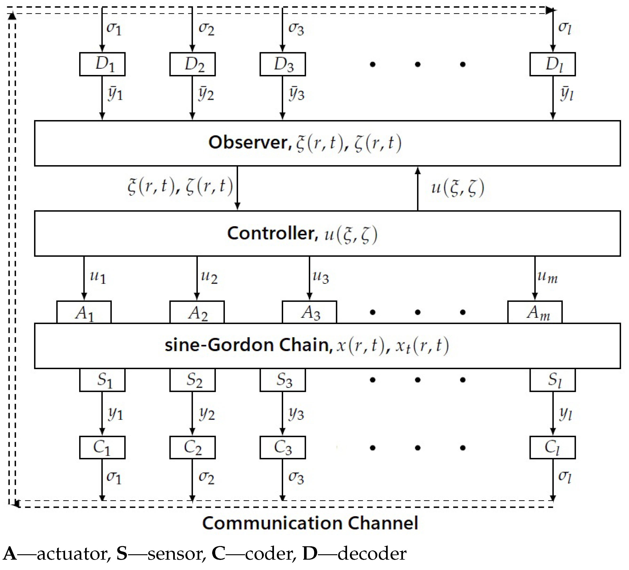
4.1. Observation Scheme with Transferring Data over the Communication Channel
4.2. Coding-Decoding Procedures
4.2.1. Time-Invariant Coder of First Order
4.2.2. Time-Invariant Coder of Full Order
4.2.3. Adaptive Coding
5. Numerical Examination Results
5.1. Quality Indices
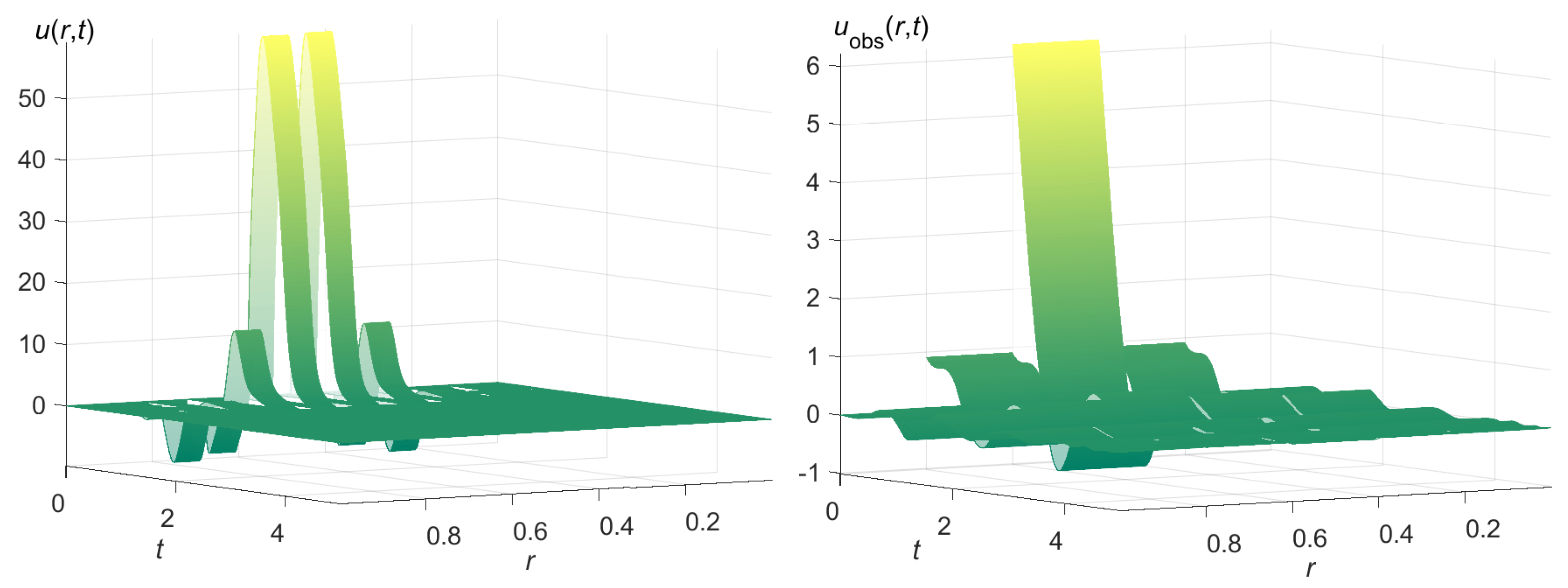
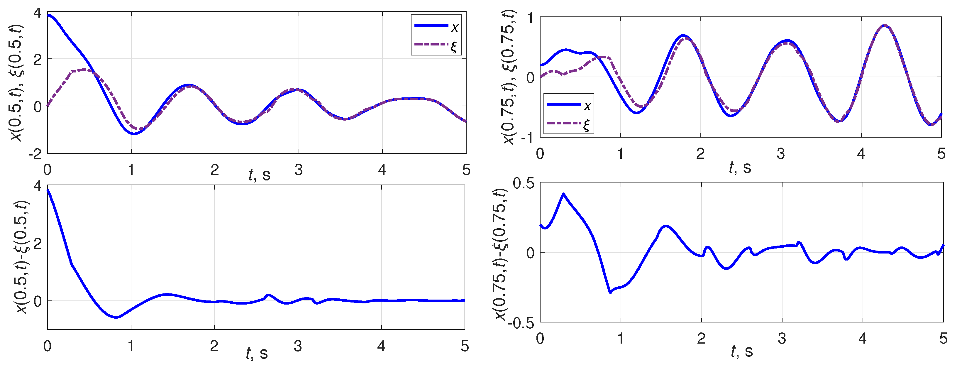
- Based on [8], the following integral-quadratic function is used to evaluate the state observation estimation accuracywhere , and .
- Since is a function, not a number, then, following the lines of [17], the corresponding quality functionals are introduced as:
- (a)
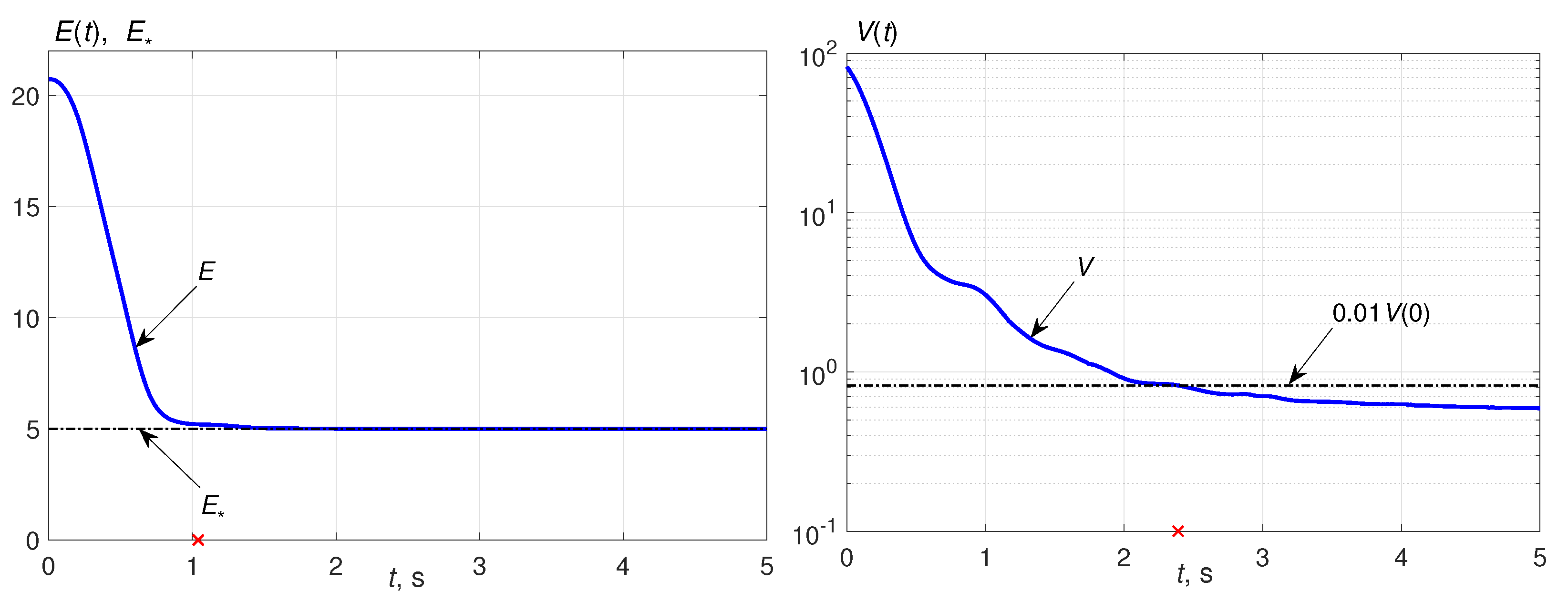
- its terminal value , where denotes the simulation time ( s in what follows);
- (b)
- trancient time , understood as the maximal instant such that . In the case of , or does not exist, then is set to ;
- Sine-Gordon chain energy given by (6) as
- The corresponding functionals are:
- (a)
- terminal value ;
- (b)
- trancient time , understood as the maximal instant such that . If this instant is greater than =30, or the given condition does not happen at all, then the quality index is set to .
5.2. Ideal Channel Case
5.2.1. Free Motion State Estimation in Ideal Channel Case
5.2.2. State-Feedback Control in Ideal Channel Case
5.3. Free Motion–State Estimation over Limited Capacity Communication Channel
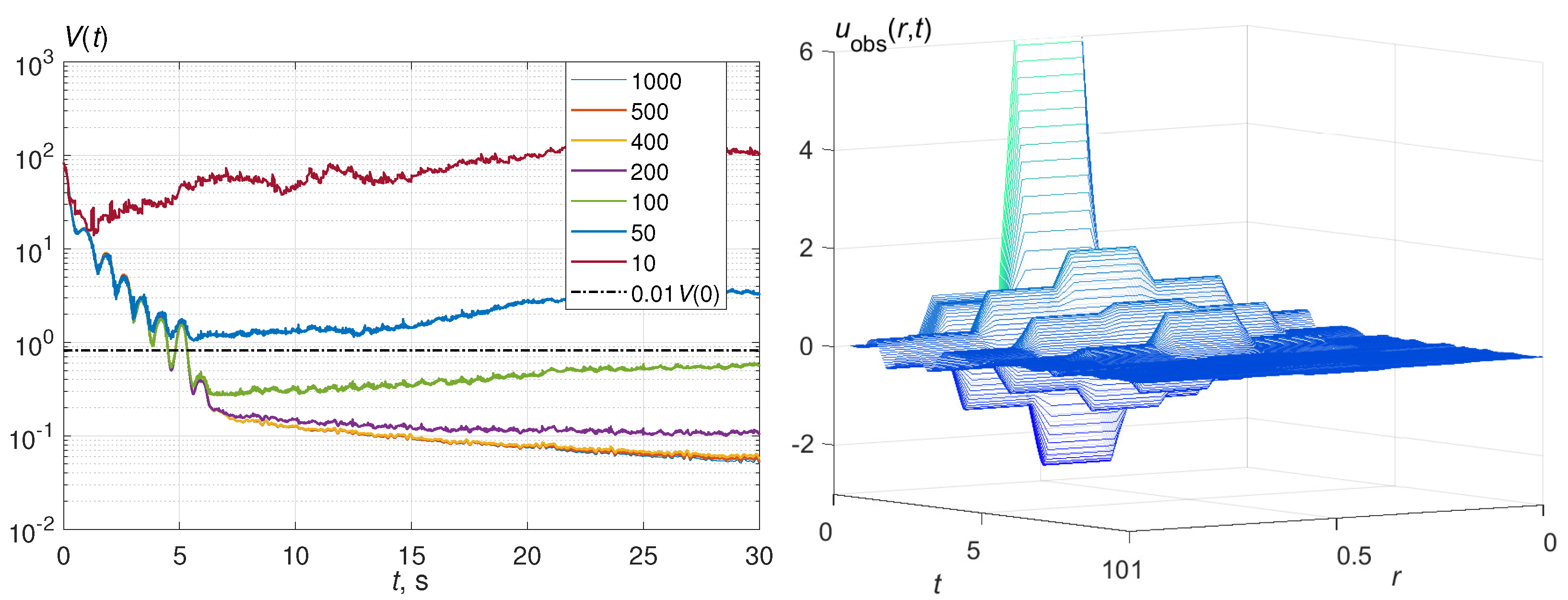
5.3.1. Free Motion State Estimation, First-Order Coder
Time-Invariant Coding
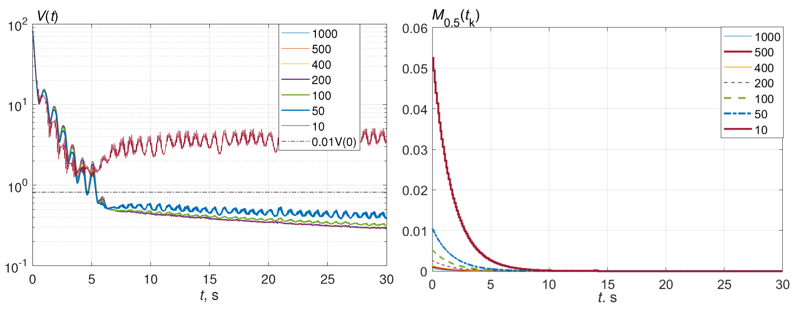
Adaptive Coding
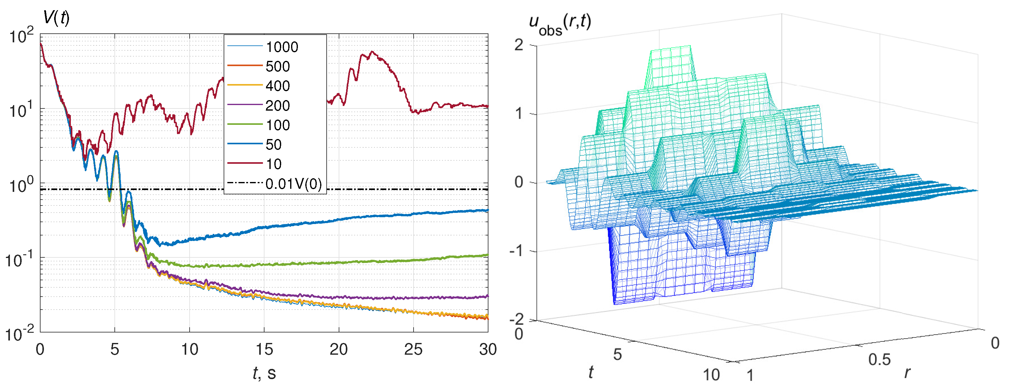
5.3.2. Free Motion State Estimation, Coder of Full Order
Time-Invariant Coding
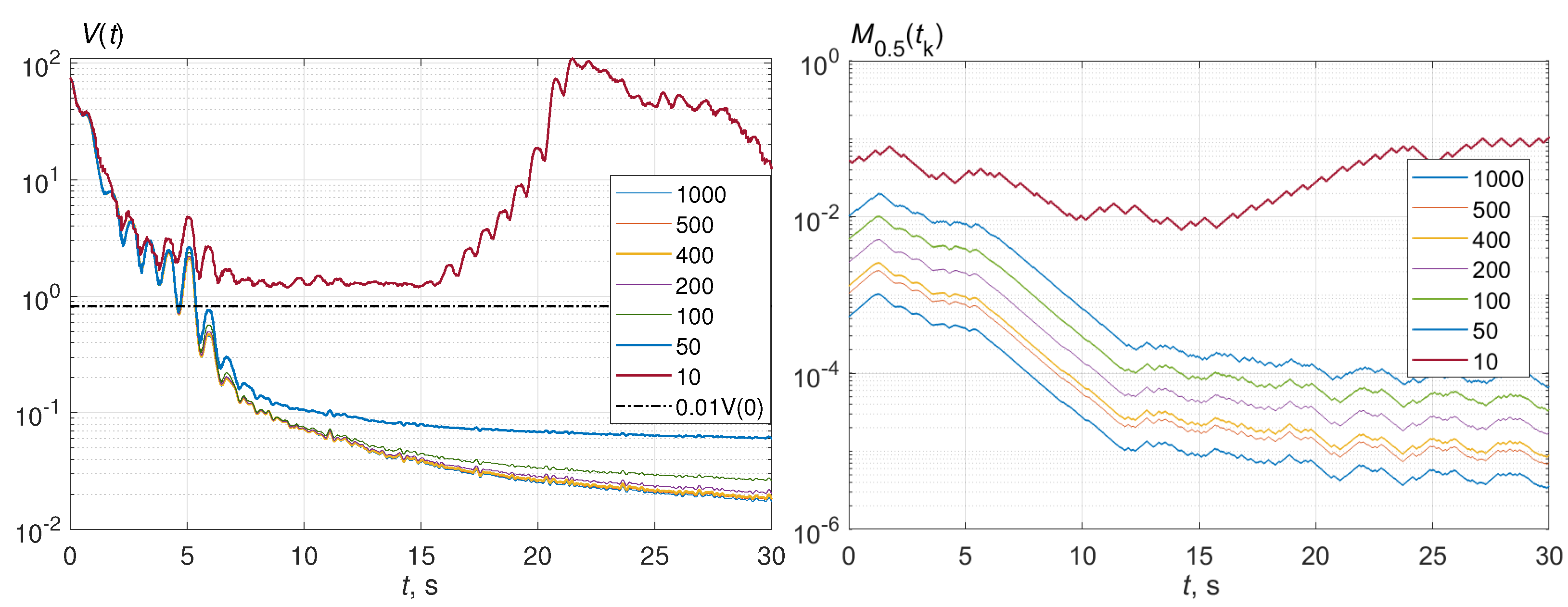
Adaptive Coding
5.4. Output Control of Energy–State Estimation over Limited Capacity Communication Channel
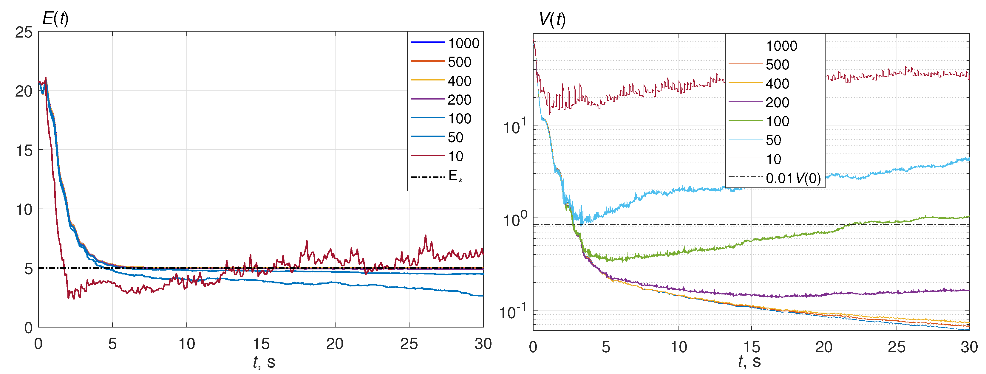
5.4.1. Output Control of Energy, First-Order Coder
Time-Invariant Coding
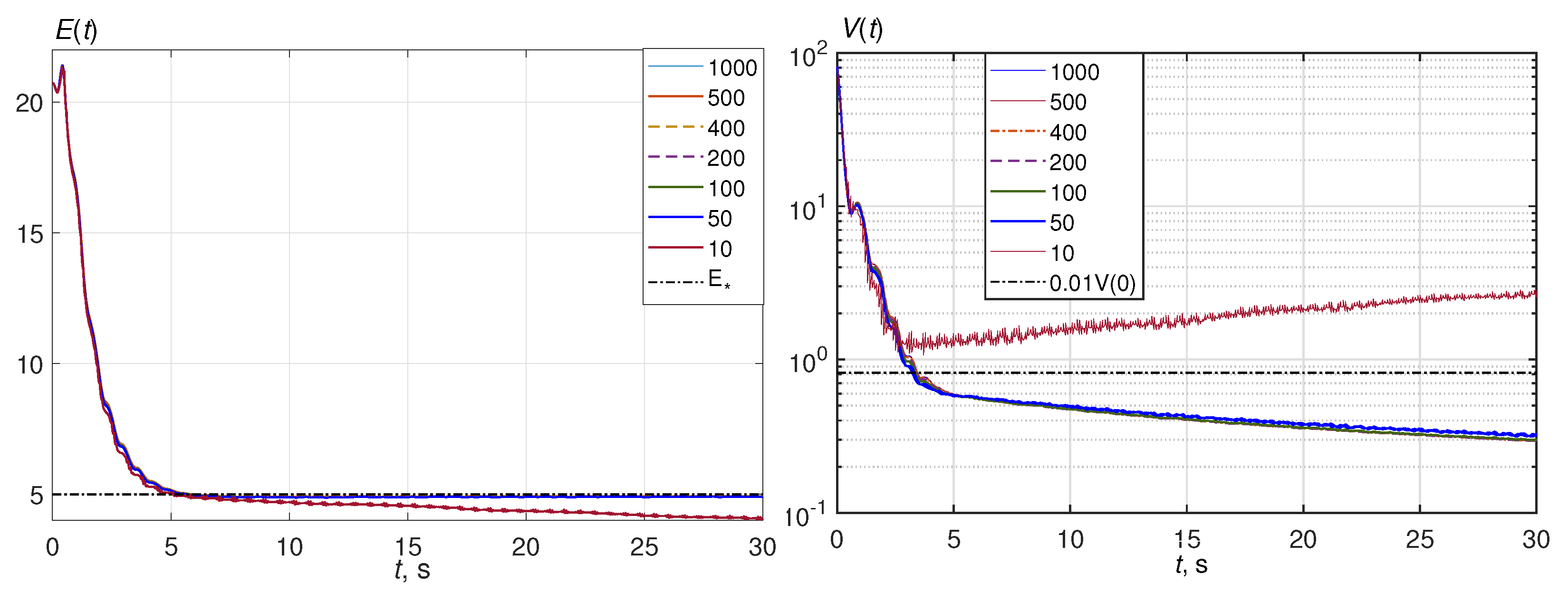
Adaptive Coding
5.4.2. Output Control of Energy, Coder of Full Order
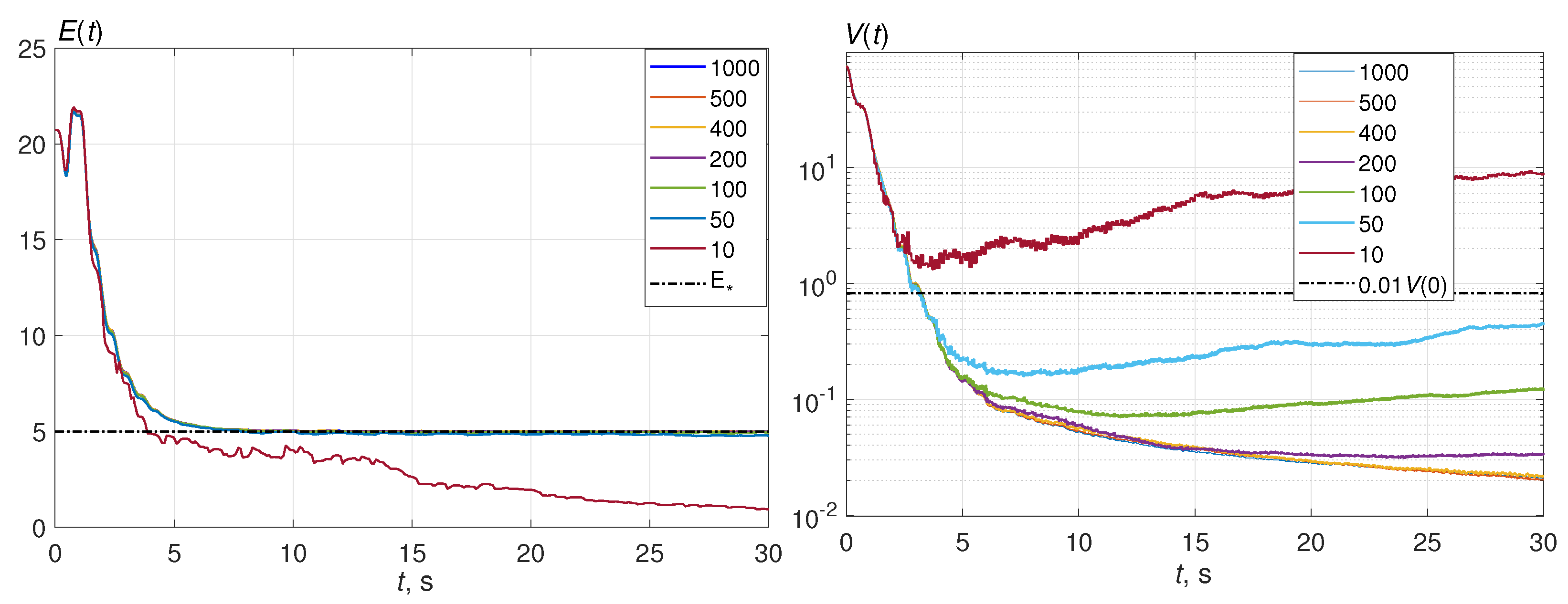
Time-Invariant Coding
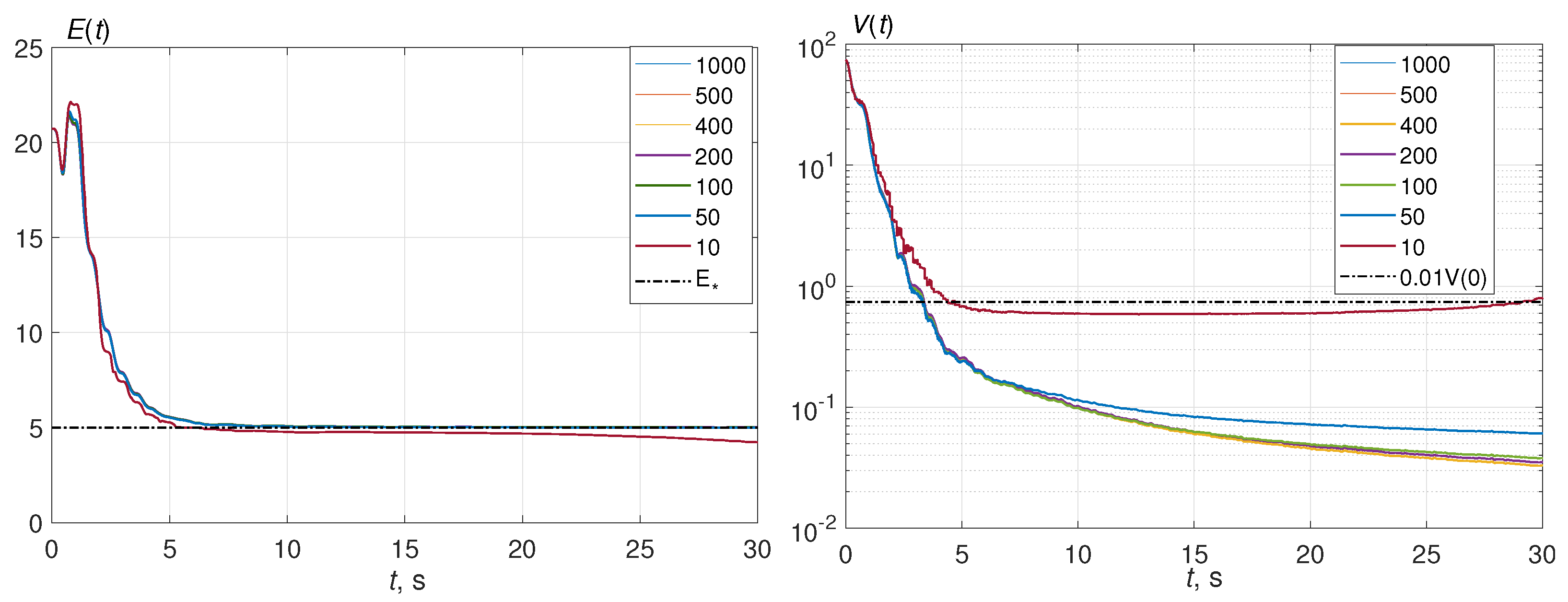
Adaptive Coding
5.5. Consolidated Results
6. Conclusions
Author Contributions
Funding
Data Availability Statement
Conflicts of Interest
Abbreviations
| 1-D | One-Dimensional |
| BVP | Boundary-Value Problem |
| LMI | Linear Matrix Inequality |
| MEMS | Microelectromechanical Systems |
| ODE | Ordinary Differential Equation |
| PDE | Partial Differential Equation |
| SG | Speed-Gradient |
| -norm of a vector x is | |
| Sobolev space | |
| Support of function —the smallest closed set containing all the points where | |
| set of nonnegative integer numbers, | |
References
- Siang, J.; Lim, M.H.; Leong, M.S. Review of vibration-based energy harvesting technology: Mechanism and architectural approach. Intern. J. Energy Res. 2018, 42, 1866–1893. [Google Scholar] [CrossRef]
- Leong, A.S.; Dey, S.; Quevedo, D.E. Transmission scheduling for remote state estimation and control with an energy harvesting sensor. Automatica 2018, 91, 54–60. [Google Scholar] [CrossRef]
- Nikpoorparizi, P.; Deodhar, N.; Vermillion, C. Modeling, Control Design, and Combined Plant/Controller Optimization for an Energy-Harvesting Tethered Wing. IEEE Trans. Control Syst. Technol. 2018, 26, 1157–1169. [Google Scholar] [CrossRef]
- Boussaid, N.; Caponigro, M.; Chambrion, T. Total Variation of the Control and Energy of Bilinear Quantum Systems. In Proceedings of the 52nd IEEE Conference on Decision and Control (CDC 2013), Firenze, Italy, 10–13 December 2013; pp. 3714–3719. [Google Scholar]
- Bonnard, B.; Caillau, J.B.; Cots, O. Energy Minimization In Two-Level Dissipative Quantum Control: The Integrable Case. Discret. Contin. Dyn. Syst. 2011, 31, 198–208. [Google Scholar]
- Mantile, A. Point interaction controls for the energy transfer in 3-D quantum systems. Intern. J. Control 2008, 81, 752–763. [Google Scholar] [CrossRef]
- Andrievsky, B.; Fradkov, A.L. Speed Gradient Method and Its Applications. Autom. Remote Control 2021, 82, 1463–1518. [Google Scholar] [CrossRef]
- Orlov, Y.; Fradkov, A.L.; Andrievsky, B. Output Feedback Energy Control of the sine-Gordon PDE Model Using Collocated Spatially Sampled Sensing and Actuation. IEEE Trans. Autom. Control 2020, 65, 1484–1498. [Google Scholar] [CrossRef]
- Fridman, E. A refined input delay approach to sampled-data control. Automatica 2010, 46, 421–427. [Google Scholar] [CrossRef]
- Fridman, E.; Seuret, A.; Richard, J.P. Robust sampled-data stabilization of linear systems: An input delay approach. Automatica 2004, 40, 1441–1446. [Google Scholar] [CrossRef]
- Balas, M.J. Toward a more practical control theory for distributed parameter systems. In Advances in Theory and Applications; Leondes, C., Ed.; Academic Press: Cambridge, MA, USA, 1982; Volume 18, pp. 361–421. [Google Scholar]
- Curtain, R.; Zwart, H. An Introduction to Infinite-Dimensional Linear Systems Theory. In Texts in Applied Mathematics; Springer: Heilderberg, Germany, 1995; Volume 21. [Google Scholar]
- Koga, S.; Karafyllis, I.; Krstic, M. Towards implementation of PDE control for Stefan system: Input-to-state stability and sampled-data design. Automatica 2021, 127, 109538. [Google Scholar] [CrossRef]
- Wang, J.W. Exponentially Stabilizing Observer-Based Feedback Control of a Sampled-Data Linear Parabolic Multiple-Input–Multiple-Output PDE. IEEE Trans. Syst. Man Cybern. 2021, 51, 5742–5751. [Google Scholar] [CrossRef]
- Katz, R.; Fridman, E. Sampled-data finite-dimensional boundary control of 1D parabolic PDEs under point measurement via a novel ISS Halanay’s inequality. Automatica 2022, 135, 109966. [Google Scholar] [CrossRef]
- Ahmed-Ali, T.; Karafyllis, I.; Giri, F. Sampled-data observers for delay systems and hyperbolic PDE–ODE loops. Automatica 2021, 123, 109349. [Google Scholar] [CrossRef]
- Andrievsky, B.; Orlov, Y.; Fradkov, A. On robustness of the speed-gradient sampled-data energy control for the sine–Gordon equation: The simpler the better. Commun. Nonlinear Sci. Numer. Simul. 2023, 117, 106901. [Google Scholar] [CrossRef]
- Cuevas-Maraver, J.; Kevrekidis, P.; Williams, F. (Eds.) The Sine-Gordon Model and Its Applications. From Pendula and Josephson Junctions to Gravity and High-Energy Physics; Springer: Cham, Switzerland, 2014. [Google Scholar]
- Kobayashi, T. Boundary feedback stabilization of the sine-Gordon equation without velocity feedback. J. Sound Vib. 2003, 266, 775–784. [Google Scholar] [CrossRef]
- Petcu, M.; Temam, R. Control for the sine-Gordon equation. ESAIM Control Optim. Calc. Var. 2004, 10, 553–573. [Google Scholar] [CrossRef]
- Kobayashi, T. Adaptive stabilization of the sine-Gordon equation by boundary control. Math. Methods Appl. Sci. 2004, 27, 957–970. [Google Scholar] [CrossRef]
- Hastir, A.; Winkin, J.J.; Dochain, D. Funnel control for a class of nonlinear infinite-dimensional systems. Automatica 2023, 152, 110964. [Google Scholar] [CrossRef]
- Dmitriev, S.V.; Shigenari, T.; Abe, K.; Vasiliev, A.A.; Miroshnichenko, A.E. Phonon emission from a discrete sine-Gordon breather. Comput. Mater. Sci. 2000, 18, 303–307. [Google Scholar] [CrossRef]
- Kivshar, Y.S.; Benner, H.; Braun, O.M. Nonlinear Models for the Dynamics of Topological Defects in Solids. In Proceedings of the Nonlinear Science at the Dawn of the 21st Century; Christiansen, P.L., Sørensen, M.P., Scott, A.C., Eds.; Springer: Berlin/Heidelberg, Germany, 2000; pp. 265–291. [Google Scholar]
- Malomed, B.A. The sine-Gordon Model: General Background, Physical Motivations, Inverse Scattering, and Solitons. In The Sine-Gordon Model and Its Applications: From Pendula and Josephson Junctions to Gravity and High-Energy Physics; Cuevas-Maraver, J., Kevrekidis, P.G., Williams, F., Eds.; Springer International Publishing: Cham, Switzerland, 2014; pp. 1–30. [Google Scholar] [CrossRef]
- Cen, J.; Correa, F.; Fring, A. Degenerate multi-solitons in the sine-Gordon equation. J. Phys. A Math. Theor. 2017, 50, 435201. [Google Scholar] [CrossRef]
- Sickotra, S. Solitons: Kinks, Collisions and Breathers. arXiv 2021, arXiv:2103.12916. [Google Scholar]
- Zhou, Q.; Ekici, M.; Mirzazadeh, M.; Sonmezoglu, A. The investigation of soliton solutions of the coupled sine-Gordon equation in nonlinear optics. J. Mod. Opt. 2017, 64, 1677–1682. [Google Scholar] [CrossRef]
- Gershenzon, N.I.; Bambakidis, G.; Skinner, T.E. Sine-Gordon modulation solutions: Application to macroscopic non-lubricant friction. Phys. D Nonlinear Phenom. 2016, 333, 285–292. [Google Scholar] [CrossRef]
- Leung, K. Mechanical properties of double-sine-Gordon solitons and the application to anisotropic Heisenberg ferromagnetic chains. Phys. Rev. B 1983, 27, 2877–2888. [Google Scholar] [CrossRef]
- Herbut, I. Dual theory of the superfluid-Bose-glass transition in the disordered Bose-Hubbard model in one and two dimensions. Phys. Rev. B-Condens. Matter Mater. Phys. 1998, 57, 13729–13742. [Google Scholar] [CrossRef]
- Temam, R. Infinite-Dimensional Dynamical Systems in Mechanics and Physics; Applied mathematical sciences; Springer: New York, NY, USA, 1997. [Google Scholar]
- Refael, G.; Demler, E.; Oreg, Y.; Fisher, D.S. Dissipation and quantum phase transitions of a pair of Josephson junctions. Phys. Rev. B-Condens. Matter Mater. Phys. 2003, 68, 214515. [Google Scholar] [CrossRef]
- Cirillo, M.; Parmentier, R.; Savo, B. Mechanical analog studies of a perturbed sine-Gordon equation. Phys. D Nonlinear Phenom. 1981, 3, 565–576. [Google Scholar] [CrossRef]
- Fradkov, A.; Andrievsky, B.; Boykov, K. Multipendulum mechatronic setup: Design and experiments. Mechatronics 2012, 22, 76–82. [Google Scholar] [CrossRef]
- Do, L.; Hurák, Z. Synchronization in the Frenkel-Kontorova Model with Application to Control of Nanoscale Friction. IFAC-PapersOnLine 2021, 54, 406–411. [Google Scholar] [CrossRef]
- Do, L.; Pučejdl, K.; Hurák, Z. Experimental Platform for Boundary Control of Mechanical Frenkel-Kontorova Model. In Proceedings of the 2022 IEEE 61st Conference on Decision and Control (CDC 2022), Cancun, Mexico, 6–9 December 2022; pp. 7618–7623. [Google Scholar] [CrossRef]
- Athans, M. Toward a practical theory for distributed parameter systems. IEEE Trans. Autom. Control 1970, 15, 245–247. [Google Scholar] [CrossRef]
- Nair, G.N.; Evans, R.J. State Estimation under Bit-Rate Constraints. In Proceedings of the 37th IEEE Conference on Decision and Control, Tampa, FL, USA, 16–18 December 1998; Volume WA09, pp. 251–256. [Google Scholar]
- Elia, N.; Mitter, S.K. Stabilization of Linear Systems with Limited Information. IEEE Trans. Autom. Control 2001, 46, 1384–1400. [Google Scholar] [CrossRef]
- Tatikonda, S.; Mitter, S. Control under communication constraints. IEEETrans. Autom. Control 2004, 49, 1056–1068. [Google Scholar] [CrossRef]
- Matveev, A.S.; Savkin, A.V. The Problem of State Estimation via Asynchronous Communication Channels with Irregular Transmission Times. IEEE Trans. Autom. Control 2003, 48, 670–676. [Google Scholar] [CrossRef]
- Nair, G.N.; Evans, R.J. Stabilizability of stochastic linear systems with finite feedback data rates. SIAM J. Control Optim 2004, 43, 413–436. [Google Scholar] [CrossRef]
- Nair, G.N.; Evans, R.J. Exponential stabilisability of finite-dimensional linear systems with limited data rates. Automatica 2003, 39, 585–593. [Google Scholar] [CrossRef]
- Nair, G.N.; Fagnani, F.; Zampieri, S.; Evans, R. Feedback control under data rate constraints: An overview. Proc. IEEE 2007, 95, 108–137. [Google Scholar] [CrossRef]
- Matveev, A.S.; Savkin, A.V. Estimation and Control over Communication Networks; Birkhäuser: Boston, MA, USA, 2009. [Google Scholar]
- Aslmostafa, E.; Ghaemi, S.; Badamchizadeh, M.A.; Ghiasi, A.R. Adaptive backstepping quantized control for a class of unknown nonlinear systems. ISA Trans. 2022, 125, 146–155. [Google Scholar] [CrossRef]
- Andrievsky, B.; Fradkov, A.L.; Peaucelle, D. Estimation and Control under Information Constraints for LAAS Helicopter Benchmark. IEEE Trans. Control Syst. Technol. 2010, 15, 1180–1187. [Google Scholar] [CrossRef]
- De Persis, C. On stabilization of nonlinear systems under data rate constraints using output measurements. Int. J. Robust Nonlinear Control 2006, 16, 315–332. [Google Scholar] [CrossRef]
- Cheng, T.M.; Savkin, A.V. Output feedback stabilisation of nonlinear networked control systems with non-decreasing nonlinearities: A matrix inequalities approach. Int. J. Robust Nonlinear Control 2007, 17, 387–404. [Google Scholar] [CrossRef]
- Brockett, R.W.; Liberzon, D. Quantized Feedback Stabilization of Linear Systems. IEEE Trans. Autom. Control 2000, 45, 1279–1289. [Google Scholar] [CrossRef]
- Liberzon, D. Hybrid feedback stabilization of systems with quantized signals. Automatica 2003, 39, 1543–1554. [Google Scholar] [CrossRef]
- Moreno-Alvarado, R.; Rivera-Jaramillo, E.; Nakano, M.; Perez-Meana, H. Simultaneous Audio Encryption and Compression Using Compressive Sensing Techniques. Electronics 2020, 9, 863. [Google Scholar] [CrossRef]
- Goodman, D.J.; Gersho, A. Theory of an Adaptive Quantizer. IEEE Trans. Commun. 1974, COM-22, 1037–1045. [Google Scholar] [CrossRef]
- Gomez-Estern, F.; Canudas de Wit, C.; Rubio, F. Adaptive delta modulation in networked controlled systems with bounded disturbances. IEEE Trans. Autom. Control 2011, 56, 129–134. [Google Scholar] [CrossRef]
- Delchamps, D.F. Stabilizing a linear system with quantized state feedback. IEEE Trans. Autom. Control 1990, 35, 916–924. [Google Scholar] [CrossRef]
- Baillieul, J. Feedback coding for information-based control: Operating near the data rate limit. In Proceedings of the 41st IEEE Conf. on Decision & Control, Las Vegas, NV, USA, 10–13 December 2002; Volume ThP02-6, pp. 3229–3236. [Google Scholar]
- De Persis, C. A Note on Stabilization via Communication Channel in the presence of Input Constraints. In Proceedings of the 42nd IEEE Conference on Decision & Control, Maui, HI, USA, 9–12 December 2003; Volume TuA06-3, pp. 187–192. [Google Scholar]
- De Persis, C. n-Bit Stabilization of n-Dimensional Nonlinear Systems in Feedforward Form. IEEE Trans. Autom. Control 2005, 50, 299–311. [Google Scholar] [CrossRef]
- Fradkov, A.L.; Andrievsky, B.; Ananyevskiy, M.S. Passification based synchronization of nonlinear systems under communication constraints and bounded disturbances. Automatica 2015, 55, 287–293. [Google Scholar] [CrossRef]
- Goodwin, G.; Lau, K.; Cea, M. Control with communication constraints. In Proceedings of the 12th Int. Conf. on Control Automation Robotics & Vision (ICARCV 2012), Guangzhou, China, 5–7 December 2012; pp. 1–10. [Google Scholar] [CrossRef]
- Paranjape, A.; Guan, J.; Chung, S.J.; Krstic, M. PDE boundary control for flexible articulated wings on a robotic aircraft. IEEE Trans. Robot. 2013, 29, 625–640. [Google Scholar] [CrossRef]
- Bialy, B.; Chakraborty, I.; Cekic, S.; Dixon, W. Adaptive boundary control of store induced oscillations in a flexible aircraft wing. Automatica 2016, 70, 230–238. [Google Scholar] [CrossRef]
- Siranosian, A.; Krstic, M.; Smyshlyaev, A.; Bement, M. Motion planning and tracking for tip displacement and deflection angle for flexible beams. J. Dyn. Syst. Meas. Control ASME 2009, 131, 1–10. [Google Scholar] [CrossRef]
- Gao, S.; Liu, J. Adaptive neural network vibration control of a flexible aircraft wing system with input signal quantization. Aerosp. Sci. Technol. 2020, 96, 105593. [Google Scholar] [CrossRef]
- Bu, X.; Qi, Q. Fuzzy Optimal Tracking Control of Hypersonic Flight Vehicles via Single-Network Adaptive Critic Design. IEEE Trans. Fuzzy Syst. 2022, 30, 270–278. [Google Scholar] [CrossRef]
- Bu, X.; Xiao, Y.; Lei, H. An Adaptive Critic Design-Based Fuzzy Neural Controller for Hypersonic Vehicles: Predefined Behavioral Nonaffine Control. IEEE/ASME Trans. Mechatronics 2019, 24, 1871–1881. [Google Scholar] [CrossRef]


| Transmission Rate, bit/s | ||||||||
| Section; Equation; Figure | Q. Fun. | 1000 | 500 | 400 | 200 | 100 | 50 | 10 |
| Section 5.3.1 | First-order Time-invariant Coder | |||||||
| Equations (26)–(29) | 0.0501 | 0.0534 | 0.0571 | 0.104 | 0.564 | 3.22 | 106 | |
| (34), (35); ; Figure 9 | 5.340 | 5.335 | 5.330 | 5.320 | ∞ | ∞ | ∞ | |
| Section 5.3.1 | First-order Adaptive Coder | |||||||
| Equations (26)–(29), (34) | 0.285 | 0.286 | 0.286 | 0.290 | 0.314 | 0.384 | 3.207 | |
| (35), (43); ; Figure 10 | 5.425 | 5.425 | 5.420 | 5.410 | 5.395 | 5.375 | ∞ | |
| Section 5.3.2 | Full-order Time-invariant Coder | |||||||
| Equations (36)–(42), (34) | 0.0151 | 0.0148 | 0.0160 | 0.0303 | 0.109 | 0.443 | 10.6 | |
| (35); ; Figure 11 | 5.382 | 5.367 | 5.357 | 5.352 | 5.351 | 5.350 | ∞ | |
| Section 5.3.2 | Full-order Adaptive Coder | |||||||
| Equations (36)–(42), (34) | 0.0173 | 0.0178 | 0.0183 | 0.0203 | 0.0261 | 0.0602 | 12.29 | |
| (35), (43); ; Figure 12 | 5.357 | 5.358 | 5.359 | 5.362 | 5.367 | 5.378 | ∞ | |
| Transmission Rate, bit/s | ||||||||
| Section; Equation | Q. Fun. | 1000 | 500 | 400 | 200 | 100 | 50 | 10 |
| Figure | ||||||||
| Section 5.4.1 | First-order Time-invariant Coder | |||||||
| 0.0618 | 0.0675 | 0.0737 | 0.166 | 1.035 | 4.501 | 34.9 | ||
| Equations (26)–(29) | 2.755 | 2.78 | 2.79 | 2.80 | ∞ | ∞ | ∞ | |
| (34), (35) | 0.009 | 0.014 | 0.027 | 0.097 | 0.502 | 2.32 | −1.450 | |
| Figure 13 | 5.157 | 5.615 | 5.133 | 5.163 | ∞ | ∞ | ∞ | |
| Section 5.4.1 | First-order Adaptive Coder | |||||||
| 0.295 | 0.295 | 0.295 | 0.296 | 0.302 | 0.328 | 2.812 | ||
| Equations (26)–(29) | 3.44 | 3.44 | 3.43 | 3.39 | 3.36 | 3.31 | ∞ | |
| (34), (35), (43) | 0.078 | 0.078 | 0.090 | 0.104 | 0.104 | 0.105 | 0.86 | |
| Figure 14 | 5.815 | 5.835 | 5.790 | 5.720 | 5.700 | 5.680 | ∞ | |
| Section 5.4.2 | Full-order Time-invariant Coder | |||||||
| 0.0210 | 0.0202 | 0.0220 | 0.0338 | 0.1225 | 0.4551 | 8.940 | ||
| Equations (36)–(42) | 3.155 | 3.190 | 3.215 | 3.225 | ∞ | ∞ | ∞ | |
| (34), (35) | 0.002 | 0.011 | 0.019 | 0.0302 | 0.075 | 0.232 | 4.06 | |
| Figure 15 | 6.538 | 6.550 | 6.555 | 6.570 | ∞ | ∞ | ∞ | |
| Section 5.4.2 | Full-order Adaptive Coder | |||||||
| 0.0324 | 0.0327 | 0.0328 | 0.0350 | 0.0379 | 0.0606 | 0.798 | ||
| Equations (36)–(42) | 3.38 | 3.38 | 3.38 | 3.37 | 3.35 | 3.31 | ∞ | |
| (34), (35), (43) | 0.0144 | 0.0143 | 0.0140 | 0.0139 | 0.0101 | −0.002 | −0.75 | |
| Figure 16 | 7.745 | 7.740 | 7.735 | 7.730 | 7.72 | 6.50 | ∞ | |
Disclaimer/Publisher’s Note: The statements, opinions and data contained in all publications are solely those of the individual author(s) and contributor(s) and not of MDPI and/or the editor(s). MDPI and/or the editor(s) disclaim responsibility for any injury to people or property resulting from any ideas, methods, instructions or products referred to in the content. |
© 2023 by the authors. Licensee MDPI, Basel, Switzerland. This article is an open access article distributed under the terms and conditions of the Creative Commons Attribution (CC BY) license (https://creativecommons.org/licenses/by/4.0/).
Share and Cite
Andrievsky, B.; Orlov, Y.; Fradkov, A.L. Output Feedback Control of Sine-Gordon Chain over the Limited Capacity Digital Communication Channel. Electronics 2023, 12, 2269. https://doi.org/10.3390/electronics12102269
Andrievsky B, Orlov Y, Fradkov AL. Output Feedback Control of Sine-Gordon Chain over the Limited Capacity Digital Communication Channel. Electronics. 2023; 12(10):2269. https://doi.org/10.3390/electronics12102269
Chicago/Turabian StyleAndrievsky, Boris, Yury Orlov, and Alexander L. Fradkov. 2023. "Output Feedback Control of Sine-Gordon Chain over the Limited Capacity Digital Communication Channel" Electronics 12, no. 10: 2269. https://doi.org/10.3390/electronics12102269