Clothoid-Based Path Planning for a Formation of Fixed-Wing UAVs

Abstract

Unmanned aerial vehicles (UAVs) are playing an increasingly crucial role in many applications such as search and rescue, delivery services, and military operations. However, one of the significant challenges in this area is to plan efficient and safe trajectories for UAV formations. This paper presents an optimization procedure for trajectory planning for fixed-wing UAV formations using graph theory and clothoid curves. The proposed planning strategy consists of two main steps. Firstly, the geometric optimization of paths is carried out using graphs for each UAV, providing piece-wise linear paths whose smooth connections are made with clothoids. Secondly, the geometric paths are transformed into time-dependent trajectories, optimizing the assigned aircraft speeds to avoid collisions by solving a mixed-integer optimal control problem for each UAV of the flight formation. The proposed method is effective in achieving suboptimal paths while ensuring collision avoidance between aircraft. A sensitivity analysis of the main parameters of the algorithm was conducted in ideal conditions, highlighting the possibility of decreasing the length of the optimal path by about 4.19%, increasing the number of points used in the discretization and showing a maximum path length reduction of about 10% compared with the average solution obtained with a similar algorithm using a graph based on random directions. Furthermore, the use of clothoids, whose parameters depend on the UAV performance constraints, provides smoother connections, giving a significant improvement over traditional straight-line or circular trajectories in terms of flight dynamics compliance and trajectory tracking capabilities. The method can be applied to various UAV formation scenarios, making it a versatile and practical tool for mission planning.

1. Introduction

Research on unmanned aerial vehicles (UAVs) has gained significant attention as an efficient alternative to manned operations. The ability to operate in hazardous environments without involving human life and lower operational costs has; made the field of UAVs one of the most rapidly growing areas. According to the Federal Aviation Administration (FAA), the number of drones and unmanned operations is expected to double by 2025 [1,2].

An area of potential development is the cooperative behavior of autonomous aircraft, acting as a group, rather than a single system. However, controlling a fleet or swarm of UAVs poses a key problem of having a (semi-)automatic calculation of suitable flight paths for all the UAVs in the formation, particularly in the presence of obstacles, no fly zones, noncooperative aircraft, and limitations from flight mechanics [3,4].

Task assignment is a critical aspect of mission planning for drone formations. It involves allocating specific tasks to individual drones to ensure the efficient and effective completion of the mission. Proper task assignment can significantly improve the overall performance of the formation by reducing redundancy, maximizing resources, and minimizing the risk of collisions. In addition, task assignment can help optimize the energy consumption of each drone, extending their flight time and reducing the need for frequent battery replacements. Therefore, careful consideration of task assignment is essential for the successful execution of complex drone missions [5,6].

Multi-UAV target assignment and path planning have become strictly related problems whose concurrent solutions must be considered. Furthermore, they can be handled as a planning problem and cooperative control as well to enable dynamic reconfiguration of the fleet in the presence of dynamic threats. In [7], the authors present a decision-theory-based solution to balance individual preferences and team needs. Together with task assignment, a Voronoi-diagram-based solution to path planning is proposed. In [8], to overcome the computational burden typical of the recalculation of the optimal results in dynamic environments, an artificial intelligence method, named simultaneous target assignment and path planning (STAPP), is presented, which uses a multiagent deep deterministic policy gradient algorithm, belonging to reinforcement learning concept.

However, route planning for UAVs is always central to cooperative behavior, and it is particularly challenging due to the complexity and nature of the environment. In general, the problem is often formulated as an optimization problem where the shortest path passes through a sequence of waypoints, considering the presence of obstacles and/or other flying vehicles and constraints deriving from the flight dynamics of the aircraft.

In the literature, many studies on 2D aerial path planning problems share algorithms and solutions with the robotics and automotive scientific communities, whereas several studies have considered the definition of 3D trajectories based on the decoupling between planar maneuvers and altitude changes [9,10].

In the last decade, several literature reviews on UAV path planning have been published [11,12,13]. In general, the existing methods can be classified into several groups: variational methods, optimal control, geometrical approaches, graph optimization, artificial potential field, and natural optimization.

In general, the variational approach to path planning produces the most natural result, but it becomes difficult to find a closed solution in complex scenarios in the presence of flight dynamics constraints and obstacles. In [14], the authors present motion planning of a hyper-redundant manipulator to overcome the typical problems of probabilistic roadmaps and graph-based optimizations in high-dimensional spaces. Another example is [15], where the path planning problem is formulated as a constrained optimization of a function that represents the total joint movement of serial manipulators with a large number of degrees of freedom.

The first alternative is optimal control [16,17,18], but it may not be effective in finding a global optimum, requiring too much computational power when dealing with nonlinear optimization algorithms.

Graph optimization is usually a good strategy, where edges are designed using geometrical methods. In such methods, the environment needs to be discretized using regular or irregular grids [19]. Other options are visibility graphs [20,21], Voronoi diagrams [22,23], rapidly exploring random trees (RRT) [24,25], tangent graphs [26], sparse tangential networks (SPARTAN) [27], and road maps [28]. To find the shortest path over graphs, some typical heuristics can be used: Dijkstra’s algorithm [29], A* algorithm [30,31], and D* algorithm [32]. However, RRT-based algorithms do not require a graph search because their graphs are trees instead of nets, so the exploration can be achieved by following the unique parent nodes to compute the solution path.

The edges of graphs can be built on pure geometrical approaches [33,34], where paths are described as a sequence of segments, arcs, or template curves.

Another commonly used approach is based on artificial potential field, which is very effective for guidance algorithms with real-time requirements [35,36,37]. However, the increase in obstacles or "potential sources" in the environment increases the probability that they are affected by singularities, which needs a strategy to avoid problems.

Natural optimization methods allow for the creation of advanced models [38,39,40,41] that are based on flight dynamics. These models involve optimizing a series of feasible maneuvers to reach a specific target point [42,43,44]. However, it should be noted that these methods tend to be slow and computationally expensive, making them more suitable for offline optimization.

The use of multiple aircraft in formation can offer several benefits from different perspectives. Initial research has been conducted on the potential advantages of flying in close formation due to fuel savings [45,46]. Some papers describe the model of fixed-wing aircraft flying in the vortex of a leader and propose the design of a control system that considers nonlinear aerodynamic coupling terms [47,48,49].

In general, coordinating a group of UAVs can improve the robustness, reliability, and performance of the entire system [50,51]. In this context, several applications are possible, such as border patrol [52], fire detection [52,53], cooperative target reconnaissance [54,55], and mobile sensor networks [56].

In general, cooperative path planning (CPP) deals with the finding of a feasible path for each UAV flying in the same environment in order to achieve a shared scope [5]. The most important difference from single UAV path planning is the cooperation variable, which makes CPP more complex. In [36], the authors dealt with a survey of the CPP problem and its constraints, focusing their attention on path coordination techniques and cooperative control methods. In [5], the authors provide a detailed review of CPP problems from the point of view of optimization techniques.

Several cooperative path planning approaches have been developed in the scientific literature [57,58,59,60,61,62,63,64,65] to address the potential applications of aircraft in close formation.

Additionally, cooperative game-theory-based approaches have been proposed to describe the behavior of aircraft in formation flight [66].

Finally, several researchers have considered control-theory-based concepts such as consensus and/or model predictive control, together with collision avoidance algorithms [67,68,69].

In this paper, a novel approach to trajectory planning for a fleet of unmanned aerial vehicles (UAVs) is presented. The contribution lies in splitting the geometric path planning problem from the collision avoidance problem, solving both tasks independently. Specifically, a combination of clothoid curves, circular arcs, and line segments is used to construct the trajectory of each UAV. This scheme was designed with two main goals in mind: to ensure compliance with both aircraft performance and environmental constraints and to identify trajectories with the minimum length.

Additionally the proposed method addresses the issue of collision avoidance between UAVs by solving a mixed-integer quadratic programming optimal control problem (MIQP) for each air vehicle in the fleet. This way, speed and acceleration along the planned trajectory can be accurately computed, thus ensuring that the aircraft avoids obstacles and collisions while maintaining its proper course.

The paper is organized as follows: In Section 2, the methodology used to build a smooth path between two prescribed routes is presented. Section 3 presents the algorithm to compute the shortest flyable path by means of a directed weighted graph, taking into account the presence of obstacles and no-fly zones. In Section 4, a distributed collision avoidance strategy is proposed, optimizing the speed of each vehicle along its path. Section 5 describes a sensitivity analysis and the numerical results, proving the effectiveness of the planning strategy, whereas in Section 6, the limitations of the proposed algorithm are summarized. Finally, in Section 7, conclusions on the present study are presented with some ideas regarding future work.

2. Single Aircraft Clothoid-Based Path Planning

A typical flight trajectory, following a series of waypoints, can be made using both straight and circular path elements [70]. However, transitioning a fixed-wing aircraft between straight and curved segments can be challenging due to the discontinuity in the path curvature at the junctions of these segments. This discontinuity needs an instantaneous change in the yaw rate (and therefore bank angle) from a zero to a nonzero value.

Flight dynamics requirements involve continuous-curvature paths with bounds on the maximum curvature and sharpness to enable accurate tracking [71,72]. Clothoids are functions that have a linear relationship between their curvature and arc length, and they can be used to reach a desired position and direction while maintaining a continuous curvature.

The equations for the spatial positions x and y as a function of the arc length s are as follows [73]:

$$x\left(s\right)=x_0+{\int }_0^{s}cos\left(\frac{1}{2}\sigma {\zeta }^2+{\kappa }_0\zeta +{\psi }_0\right)d\zeta$$

(1)

$$y\left(s\right)=y_0+{\int }_0^{s}sin\left(\frac{1}{2}\sigma {\zeta }^2+{\kappa }_0\zeta +{\psi }_0\right)d\zeta$$

(2)

where $\sigma$ represents the curvature change rate or sharpness, ${\kappa }_0$ is the initial curvature, ${\psi }_0$ is the initial heading, and $\zeta$ gives the integration variable. Multiple clothoids can be combined into a spline to create a continuous curvature path [74,75,76,77] by matching the curvature at the junctions of clothoid segments.

To establish the limits for curvature and sharpness, the maximum bank angle ${\varphi }_{max}$ and the bank angle rate ${\dot{\varphi }}_{max}$ must be taken into account. The maximum path curvature can be calculated based on the speed v, gravity g, and the maximum bank angle ${\varphi }_{max}$ [78]. Once the maximum path curvature is determined, the maximum sharpness is found by differentiating the curvature function with respect to time.

$${\kappa }_{max}=\frac{g}{v^2}tan\left({\varphi }_{max}\right)$$

(3)

$${\sigma }_{max}=\frac{g}{v^2}{\dot{\varphi }}_{max}{sec}^2\left({\varphi }_{max}\right)$$

(4)

The curvature of a clothoid is considered linear along a curve. Therefore, the minimum and maximum curvature occur at the tips of a clothoid segment.

Flyable Path between Two Directions

Consider two straight lines $r_j$ and $r_k$ intersecting at a point Q. Such lines define the desired heading of an aircraft flying over them, ${\psi }_j$ and ${\psi }_k$, respectively.

A flyable path between two intersecting straight lines can be computed by two clothoids and an arc, if necessary. The presence of such a circular arc must be considered by taking into account any constraint of the aircraft on the roll angular speed. The last definition can be considered an alternative to the Dubins path [79] by smoothing the tips of the circular arc, to avoid discontinuities on the curvature.

The curvature of the flyable path rises from zero to $k_{max}$ to obtain the transition between the straight trajectory given by $r_j$ and the circular arc; after that, the curvature remains constant until the following transition between the arc and the final direction $r_k$, with the curvature decreasing between $k_{max}$ and zero.

Procedure 1. Clothoid-based flyable path between two directions

• STEP 1. Firstly, compute the angles ${\psi }_j$ and ${\psi }_k$ between an arbitrary axis and $r_j$ and $r_k$, respectively.
• STEP 2. Assuming $\mathsf{\Delta }\psi =\left|{\psi }_k-{\psi }_j\right|$, ${\kappa }_{max}$ (the maximum curvature), and ${\sigma }_{max}$ (the maximum sharpness), it is possible to compute $\mathsf{\Delta }{s}_{max}=2\ast {\kappa }_{max}/{\sigma }_{max}$ as the length of a virtual curve with the maximum sharpness and maximum curvature. It is worth noting that it is called virtual because the heading change constraint has not yet been considered.
• STEP 3. The area of the trapezium with major base $\mathsf{\Delta }{s}_{max}$, minor base l as the length of the circular arc, and height ${\kappa }_{max}$ must be equal to $\mathsf{\Delta }\psi$. The minor base can be computed as:

  $$l=\frac{\mathsf{\Delta }\psi }{{\kappa }_{max}}-\frac{\mathsf{\Delta }{s}_{max}}{2}$$
  If $l>0$, the path includes a circular arc with curvature ${\kappa }_{max}$. If $l=0$, then the path includes only two clothoids, and the maximum curvature ${\kappa }_{max}$ is reached in the middle point. If $l<0$, the path includes only two clothoids that do not reach the maximum curvature.
• STEP 4. Starting from the intersection point Q, if $l>0$, a half-circle arc can be computed using (1) and (2), with $\sigma =0$, $\kappa ={\kappa }_{max}$ and $s\in \left[0,\frac{l}{2}\right]$; if $l=0$ ($l<0$), the clothoid curve can be computed using (1) and (2), with $\sigma =-{\sigma }_{max}$ and $\kappa ={\kappa }_{max}$ ($\kappa ={\sigma }_{max}\ast \frac{\mathsf{\Delta }{s}_{max}}{2}$). These segments represent the second half of the overall curve. The first part can be computed by mirroring the results with respect to the median line between the considered directions.
• STEP 5. The curve must be moved in order to be tangent to both the assigned directions.

3. Single Aircraft Graph Construction

In this section, the path planning algorithm for each vehicle is presented. For each UAV, consider a starting point A and a target point B, with prescribed directions ${\mathbf{d}}_A$ and ${\mathbf{d}}_B$, respectively. Assume the presence of $N_o$ polygonal obstacles in the flight space. The goal of the path planning problem is to find the shortest flyable path, connecting the starting and target points in accordance with the initial and final directions ${\mathbf{d}}_A$ and ${\mathbf{d}}_B$, respectively.

Problem 1.

Given the starting and target points A and B, with prescribed directions ${\mathbf{d}}_A$ and ${\mathbf{d}}_B$, respectively, and $N_o$ polygonal obstacles, find the shortest flyable path connecting A to B with initial direction ${\mathbf{d}}_A$ and approaching direction ${\mathbf{d}}_B$.

The solution to Problem 1 is NP-hard [70]. Consequently, in order to obtain a suboptimal solution in a reasonable time, the problem can be simplified by discretizing the flight space in prescribed admissible routes passing through a given number of points. This strategy allows converting the trajectory planning problem into a minimum cost search problem within a graph $\mathbb{G}=\{\mathcal{N},\mathcal{E}\}$. The node set $\mathcal{N}$ contains any waypoint that can be overflown by the optimal path, while the arc set $\mathcal{E}$ is composed of straight segments and clothoid-based paths that are used to build the flight trajectory. Each arc of the graph is weighted with the curve length used to connect the nodes.

Let ${\mathcal{S}}_p$ denote the set of edges composing obstacle ${\mathfrak{P}}_p$ with $p=1,\dots ,N_o$.

$\mathcal{D}=\{{\mathbf{d}}_1^{+},{\mathbf{d}}_1^{-}\dots ,{\mathbf{d}}_n^{+},{\mathbf{d}}_n^{-}\}$ is the set of the prescribed directions, where the superscripts ${(·)}^{+}$ and ${(·)}^{-}$ denote the positive and negative orientations, respectively. On the other hand, for each edge $e_j$, with $e_j\in {\bigcup }_{p=1}^{N_o}{\mathcal{S}}_p$, consider the set $\mathcal{D}\left(e_j\right)=\{{\mathbf{d}}_{ej}^{+},{\mathbf{d}}_{ej}^{-}\}$ composed of the positive and negative directions, parallel to $e_j$.

Definition 1.

The set of admissible directions is

$$\tilde{\mathcal{D}}=\mathcal{D}\cup \left(\bigcup _{p=1}^{N_o}\bigcup _{e_j\in {\mathcal{S}}_p}\mathcal{D}\left(e_j\right)\right)$$

(5)

Definition 2.

An admissible route $r_k$ is an oriented straight line having direction ${\mathbf{d}}_k^{*}\in \tilde{\mathcal{D}}$.

Consider a grid of m points $C_i$ in the flight space $\mathcal{W}=\{C_1\dots C_m\}$.

Definition 3.

The set ${\mathcal{R}}_{C_i}$ of admissible routes passing through the point $C_i$, is composed of $\tilde{n}=card\left(\tilde{\mathcal{D}}\right)$-oriented straight lines, each of them having a direction equal to ${\mathbf{d}}_j^{*}\in \tilde{\mathcal{D}}$:

$${\mathcal{R}}_{C_i}=\left\{r_{j_i}:r_{j_i}\Vert {\mathbf{d}}_j^{*},\forall {\mathbf{d}}_j^{*}\in \tilde{\mathcal{D}}\right\}$$

(6)

For A and B, the sets of admissible routes, ${\mathcal{R}}_A$ and ${\mathcal{R}}_B$ respectively, consist of a unique oriented straight line having an orientation equal to the directions ${\mathbf{d}}_A$ and ${\mathbf{d}}_B$, respectively.

Definition 4.

The overall set of admissible routes $\mathcal{R}$ is:

$$\mathcal{R}={\mathcal{R}}_A\cup {\mathcal{R}}_B\cup \left\{r_{k_i}:r_{k_i}\in \left(\bigcup _{i=1}^m{\mathcal{R}}_{C_i}\right)\right\}$$

(7)

Considering two straight lines $r_{j_i}$ and $r_{k_l}$, belonging to $\mathcal{R}$, with the intersection point Q, it is possible to build two clothoid-based paths ${\mathrm{\Gamma }}_{j_i,k_l}^Q$ and ${\mathrm{\Gamma }}_{k_l,j_i}^Q$. ${\mathrm{\Gamma }}_{j_i,k_l}^Q$ allows the vehicle to pass from the route $r_{j_i}$ to $r_{k_l}$, whereas ${\mathrm{\Gamma }}_{k_l,j_i}^Q$ changes direction from $r_{k_l}$ to $r_{j_i}$.

This strategy permits the decomposing of the workspace into a huge number of routes ($m·\tilde{n}+2$); consequently, it requires the construction of a large number of clothoid-based paths. However, it is worth noticing that for each couple of nonparallel directions ${\mathbf{d}}_j^{*}$ and ${\mathbf{d}}_k^{*}$, it is possible to build two a priori clothoid-based paths ${\mathrm{\Gamma }}_{j,k}$ and ${\mathrm{\Gamma }}_{k,j}$. Consequently, the overall computational burden can be reduced to the calculation of $\frac{\left(\tilde{n}+1\right)\left(\tilde{n}+2\right)}{2}$ clothoid-based paths that are successively translated in any intersection point between every couple of routes $r_{j_i}$ and $r_{k_l}$, with $i,l=1,\dots ,m$.

Each clothoid-based path, ${\mathrm{\Gamma }}_{j_i,k_l}^Q$, is defined by an initial point $T_{j_i}^{Q,in}$ and a final point $T_{k_l}^{Q,out}$, with $T_{j_i}^{Q,in}$ belonging to the initial admissible route $r_{j_i}$ and $T_{k_l}^{Q,out}$ belonging to the route $r_{k_l}$.

$T_{j_i}^{Q,in}$ and $T_{k_l}^{Q,out}$ are nodes of the graph $\mathbb{G}$, i.e., $T_{j_i}^{Q,in},T_{k_l}^{Q,out}\in \mathcal{N}$. The arc set $\mathcal{E}$ is composed of the clothoid-based paths from the points $T_{j_i}^{Q,in}$ to $T_{k_l}^{Q,out}$ plus the straight segments that connect the points $T_{k_l}^{Q,out}$ and $T_{k_l}^{O,in}$ on the same route $r_{k_l}$.

The algorithm used for graph construction is reported as a pseudo-code in Algorithm 1. Once the graph is built, the shortest trajectory is computed by using Dijkstra method [80].   

Algorithm 1 Pseudo-code for graph generation

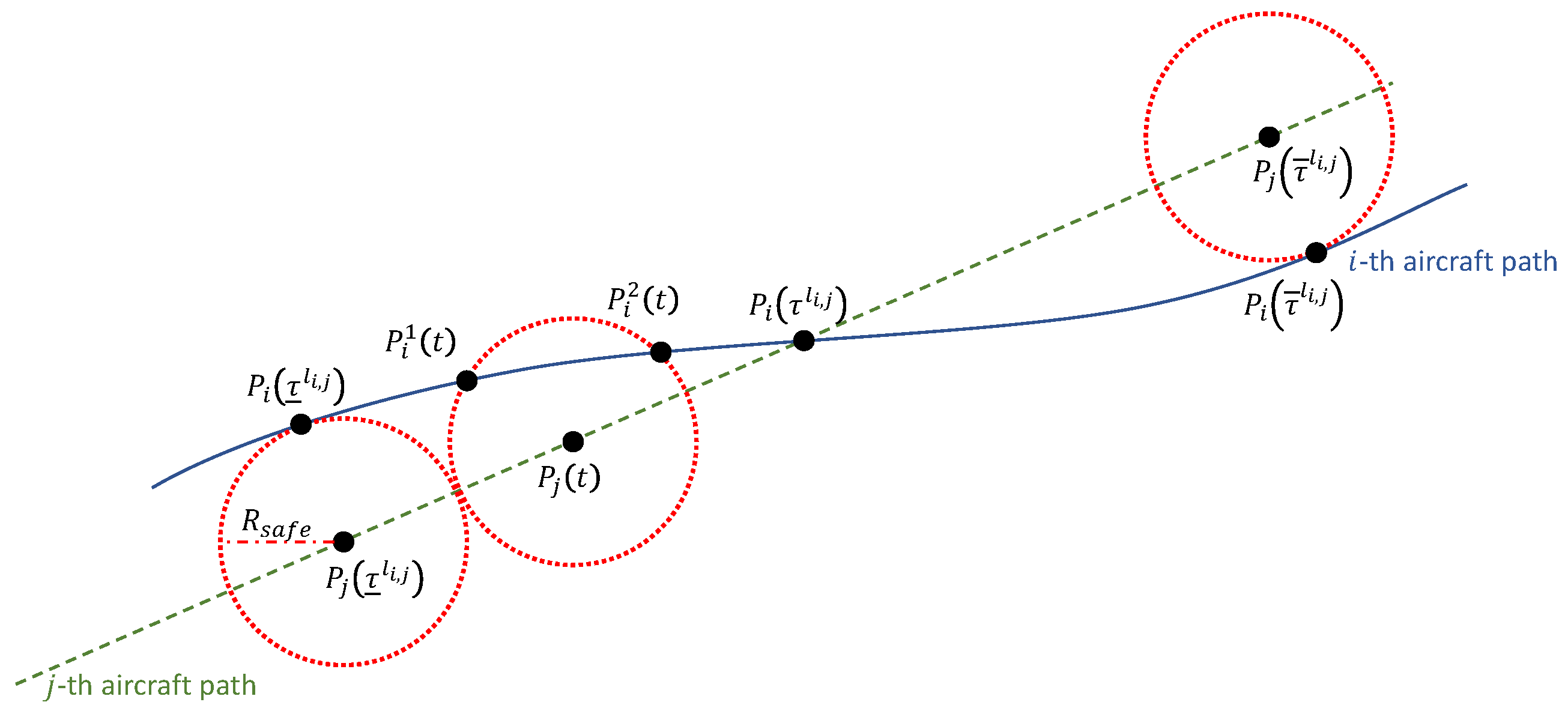
4. Multivehicle Path Planning and Collision Avoidance

In this section, the applicability of these algorithms to a fleet of UAVs is described.

Consider $N_v$ fixed-wing aircraft each flying from a given departure point to a given target point.

The mission planning starts by constructing a graph for each UAV, taking into account its specific starting and ending points, as well as the fixed departure and arrival directions. Being routes shared between aircraft, clothoid curves can be precalculated by the algorithm to be later used in any graph construction.

For each UAV in the swarm, the algorithm computes the intersection points between the assigned directions, then reconstructs the graph based on these points and the precomputed clothoids.

However, the resulting trajectories, in many cases, present several geometrical intersections that can be possible collisions between UAVs. A solution can be the generation of a shortest path tree [81] for each aircraft, building several suboptimal alternative paths, probably leading to significant deviations from the optimal trajectory.

Once the flight level is assigned, to prevent collisions between the unmanned aerial vehicles (UAVs) in a given fleet, as well as collisions with noncooperative aircraft (intruders), ensuring that UAVs arrive at waypoints and targets on scheduled time, the speed profiles of all vehicles along their flight paths can be optimized [9]. Speeds must be chosen within admissible ranges, depending on the type of UAV. For UAVs with hovering capabilities, speeds can range from zero to their maximum speed. For fixed-wing UAVs, allowable speeds are between stall speed and maximum speed.

Modeling the aircraft as a mass point subject to constraints on maximum and minimum accelerations and speeds ($a_{max}$, $a_{min}$, $v_{max}$, and $v_{min}$, respectively) along the flight path, assuming the trajectories of known or predetermined intruders, such that they gradually change in relation to the aircraft maneuvering capabilities and response times, aircraft motion can be formulated along the path as a single degree of freedom model in the form:

$$\dot{\mathit{q}}\left(t\right)=\left[\begin{array}{cc}0& 1\\ 0& 0\end{array}\right]\mathit{q}\left(t\right)+\left[\begin{array}{c}0\\ 1\end{array}\right]u\left(t\right)=\mathit{A}\mathit{q}\left(t\right)+\mathit{B}u\left(t\right)$$

(8)

where $\mathit{q}\left(t\right)={\left[s\left(t\right),v\left(t\right)\right]}^T$ is the state vector, s is the curvilinear abscissa indicating the position along the flight path, v is the aircraft speed, and u is the control signal in terms of desired acceleration tangent to the path.

It is worth noting that the use of a kinematic model neglects the dynamics of the UAV, but it can be considered a reasonable approximation for a vehicle with a control system capable of following a trajectory, taking into account flight conditions and tracking error.

It is therefore assumed that such a control system is able to guide the UAV while maintaining minimal deviation from the planned trajectory. This way, the anticollision problem can be approximated as a one-dimensional problem on curvilinear abscissa.

Problem 2.

Consider an aircraft i, described by (8), flying along a path ${\mathit{P}}_i\left(t\right)$ within the time interval $\left[{\tau }_0,{\tau }_f\right]$. The objective of the collision avoidance problem is to determine an optimal input function $u_i{\left(t\right)}^{*}$ that ensures a specified safety distance, $R_{safe}$, between i and every aircraft j in the fleet.

This can be formulated as a constrained optimal control problem, as follows:

$$mi{n}_u{\int }_{{\tau }_0}^{{\tau }_f}\left[{\left(\mathit{q}\left(t\right)-{\mathit{q}}_r\left(t\right)\right)}^T\mathbb{Q}\left(\mathit{q}\left(t\right)-{\mathit{q}}_r\left(t\right)\right)+u{\left(t\right)}^T\mathbb{R}u\left(t\right)\right]dt$$

(9)

$$s.t.\left\{\begin{array}{c}{v}_{min}\le v\le v_{max}\\ u_{min}\le u\le u_{max}\\ R_{i,j}\left(t\right)\ge R_{safe}\forall j\in \left[1,N_v\right],\forall t\in \left[{\tau }_0,{\tau }_f\right]\end{array}\right.$$

(10)

where ${\mathit{q}}_r\left(t\right)$ represents the desired state, $\mathbb{Q}$ and $\mathbb{R}$ are suitable weight matrices, and $R_{i,j}$ is the distance between the aircraft. However, the last constraint in (10) cannot be easily modeled due to the 1D nature of the described state.

To overcome this difficulty, ensuring the problem is linear and 1D, the collision avoidance constraint must be rewritten by precalculating possible collisions between aircraft flying at a fixed speed. A discrete set of constraints can be defined to ensure that the aircraft position does not fall within a moving separation circle centered at the jth aircraft position and having radius $R_{safe}$.

Such set can be computed by assuming a sufficient number of control time instants t, such that the relative distance between the two aircraft does not change more than a fixed fraction ${ϵ}_{safe}$ (e.g., 0.1) of the safety radius $R_{safe}$ during one step.

To generalize the problem of collision avoidance, consider only two UAVs: i and j. With reference to Figure 1, consider an arbitrary intersection l at time instant ${\tau }^{l_{i,j}}$ between the trajectories of the aircraft. A time interval $\left[{\underline{\tau }}^{l_{i,j}},{\overline{\tau }}^{l_{i,j}}\right]$ can be defined where the distance between aircraft $R_{i,j}\left(t\right)$ is less or equal to the prescribed $R_{safe}$ with $t\in \left[{\underline{\tau }}^{l_{i,j}},{\overline{\tau }}^{l_{i,j}}\right]$. That is, the aircraft i is in the separation circle centered on position ${\mathit{P}}_{\mathit{j}}\left(t\right)$ of the jth UAV.

$$R_{i,j}\left({\underline{\tau }}^{l_{i,j}}\right)=R_{i,j}\left({\overline{\tau }}^{l_{i,j}}\right)=R_{safe}$$

(11)

$$R_{i,j}\left(t\right)\le R_{safe}\forall t\in \left[{\underline{\tau }}^{l_{i,j}},{\overline{\tau }}^{l_{i,j}}\right]$$

(12)

In order to avoid collisions, it is necessary for aircraft i to always be outside the separation circle, that is, in terms of curvilinear abscissa:

$$s_i\left(t\right)\le s_{i,j}^1\left(t\right)\mathrm{or}{s}_i\left(t\right)\ge s_{i,j}^2\left(t\right)\forall t\in \left[{\underline{\tau }}^l,{\overline{\tau }}^l\right]$$

(13)

Here, $s_{i,j}^1$ and $s_{i,j}^2$ represent the curvilinear abscissa at the intersection points between the trajectory of vehicle i and the separation circle centered at $P_j\left(t\right)$, respectively, depicted as $P_i^1\left(t\right)$ and $P_i^2\left(t\right)$, respectively, in Figure 1.

However, in the event of a potential collision, vehicle i has only two viable courses of action: accelerating and passing ahead of vehicle j or decelerating to pass behind it.

Consider a sufficiently large scalar M and a variable ${\beta }_{l_{i,j}}$ such that:

$$\begin{array}{c}{\beta }_{li,j}\in \{0,1\},\hfill \end{array}$$

(14)

with $l_{i,j}\in {\mathcal{L}}_{i,j}$ being the set of intersections between the paths related to aircraft i and aircraft j.

The constraints in (13) can be reformulated as follows:

$$\begin{array}{c}{s}_i\left(t\right)\le s_{i,j}^1\left(t\right)+{\beta }_{l_{i,j}}·M\hfill \\ s_i\left(t\right)\ge s_{i,j}^2\left(t\right)-(1-{\beta }_{l_{i,j}})·M\hfill \end{array} \forall t\in \left[{\underline{\tau }}^{l_{i,j}},{\overline{\tau }}^{l_{i,j}}\right]$$

(15)

The solution to the overall collision avoidance problem for the entire fleet is found by sequentially solving the MIQP defined by (9), (10), (14), and (15) for each aircraft given an assigned order, where each vehicle takes into account the trajectories of the aircraft with higher hierarchical levels only.

5. Results

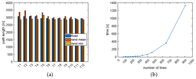
5.1. Test Case #1: Sensitivity Analysis in Unconstrained Environment

This test case focuses on singl- aircraft path planning, being part of the overall multiaircraft procedure presented in the paper.

In particular, a sensitivity analysis is shown to illustrate the relationship between the operating parameters of the proposed path planning algorithm and the obtained solution, with a focus on path quality in terms of minimum length and computational burden.

To have a benchmark, a comparison was made with results obtained by using the algorithm proposed in [28], where the graph was built upon a certain number of random directions.

The scenario considered in the first comparison has no obstacles, to exploit the capability of the proposed procedure in finding a path between two points given the departure and arrival directions.

The scenario parameters considered in this simulation are listed in

Table 1. Test case #1: scenario parameters.

Description	Value
Starting Point $\mathit{A}$	(0,0) m
Departure Heading ${\mathit{\psi }}_{\mathit{A}}$	$\pi /4$
Minimum Turning Radius	260 m
Target Point $\mathit{B}$	(2000,2000) m
Arrival Heading ${\mathit{\psi }}_{\mathit{B}}$	$\pi /8$

, giving the location of the starting and target points as well as the prescribed departure and target directions. As shown in

Table 2. Scenario #1: algorithm parameters.

Configuration Name	Number of Points m	Number of Directions n
T1	8	2
T2	8	4
T3	8	6
T4	8	12
T5	16	2
T6	16	4
T7	16	6
T8	16	12
T9	32	2
T10	32	4
T11	32	6
T12	32	12

, different set of operating parameters, obtained by increasing the number of points m and the number of directions n, were defined and used in the running algorithms.

Figure 2a presents a comparison between the proposed procedure and the randomly generated graphs suggested by [28], using the same number of lines. To ensure a meaningful comparison, the random-based algorithm was repeated 10 times for each test, displaying the minimum and average path lengths. As shown in Figure 2a, an expected outcome of increasing the number of lines for the graph construction is the improvement in the solution quality in terms of minimum length, both in fixed- and random-based graphs. However, increasing the number of lines beyond 500/600 does not yield further improvements in the solution quality, whereas, as illustrated in Figure 2b, the computational time significantly increases. Furthermore, in this simple scenario, the resulting path, is almost insensitive to the number of directions; the path length is mainly dependent on the number of grid points. While the proposed algorithm cannot always find the best path, it consistently provides better solutions than the average one found by the random-based algorithm, showing a maximum path length reduction of about 10%. Figure 3 shows the optimal trajectories with three grid configurations. As illustrated, increasing the number of points m gives more options to the algorithm to further improve the path. However, the results obtained with configurations T5 and T9 are equal, while using configuration T1 results in a longer path. According to this test case, it can be inferred that configurations T5 and T9 result in a solution percentage improvement of 4.19% compared with configuration T1.

It is worth noting that the trivial minimum length path, i.e., the straight segment connecting points A and B, is not allowed because trajectory must be compliant with the departure and target directions.

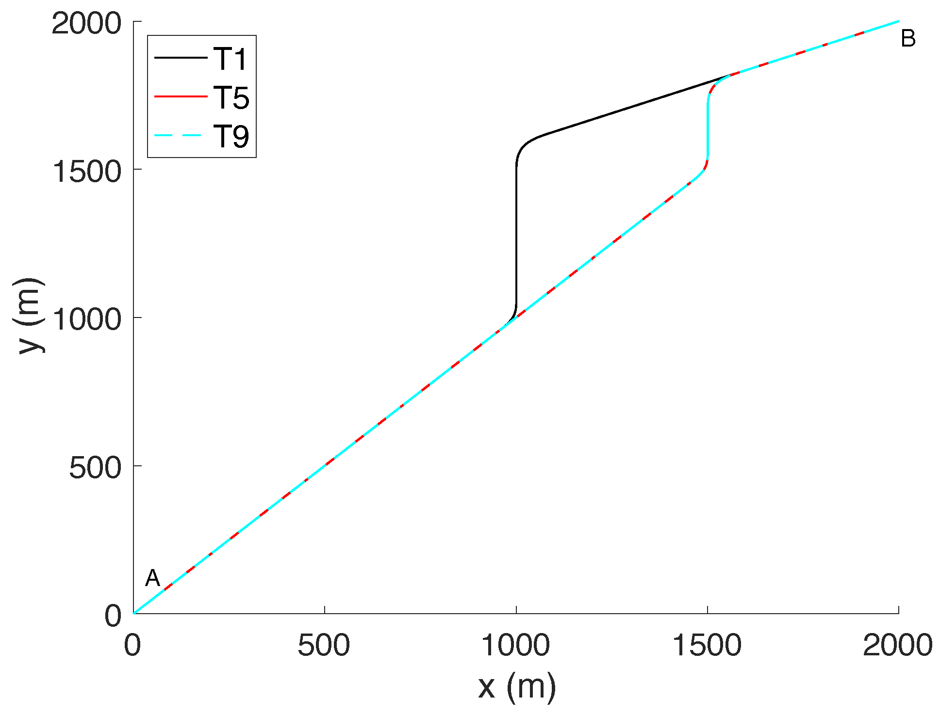
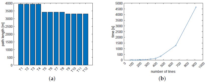
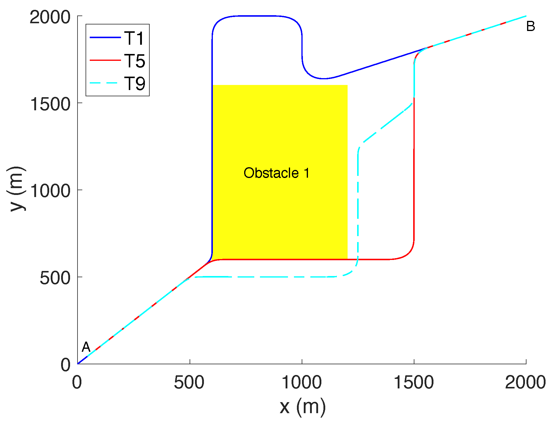
5.2. Test Case #2: Sensitivity Analysis in Constrained Environment

The scenario considered in the second presents one obstacle at the center of the considered box to demonstrate the capability of the proposed procedure to find a path between two points with given departure and arrival directions, avoiding the obstacle.

The positions of the starting and target points as well as the prescribed directions and obstacle corner points are listed in

Table 3. Test case #2: scenario parameters.

Description	Value
Starting Point $\mathit{A}$	(0,0) m
Departure Heading ${\mathit{\psi }}_{\mathit{A}}$	$\pi /4$
Target Point $\mathit{B}$	(2000,2000) m
Arrival Heading ${\mathit{\psi }}_{\mathit{B}}$	$\pi /8$
Minimum Turning Radius	260 m
Obstacle ${\mathfrak{P}}_1$ corner points	(600,600) m (1200,600) m (1200,1600) m (600,1600) m

.

As in #1, several configuration parameters were considered, as shown in Table 2.

Figure 4a shows the path length obtained with the different configurations of parameters. The results confirmed the expected solution improvement by increasing the number of grid points. However, the simple selected scenario did not yet allow for highlighting the importance of the number of directions in the trajectory optimization process. The presence of some predefined directions, deriving from the departure and arrival directions and from the edges of the polygonal obstacle, makes the additional directions defined in the table unnecessary. As expected, Figure 4b shows how the computational burden increases with a higher number of graph points and routes.

Finally, Figure 5 shows the scenario configuration and the optimal trajectories with different grid configurations. The best path was obtained using the T9 configuration. It is worth noting that the use of the T1 configuration results in a trajectory with many unnecessary turns lengthening the path due to the lack of having enough points to better fit the scenario.

In this second test case, it could be observed that configuration T5 yields a solution improvement of 13% over configuration T1, while configuration T9 gives a reduction of 15% in trajectory length.

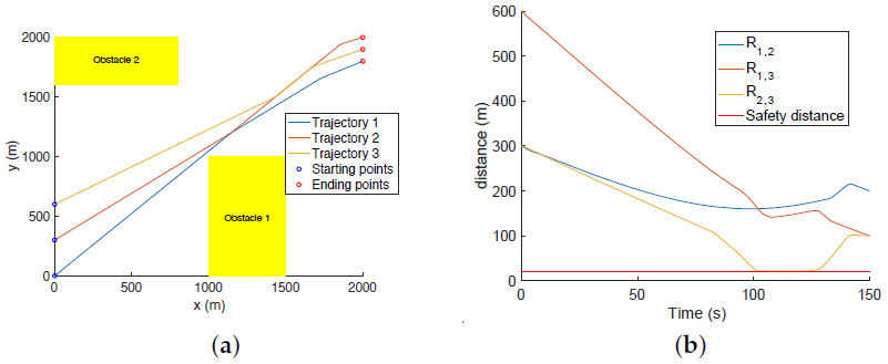
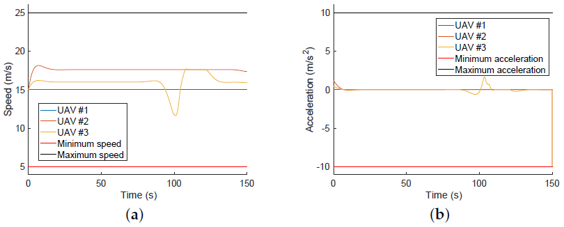
5.3. Test Case #3: Trajectory Planning for a Fleet of 3 UAVs

The first multivehicle scenario presents two nearby obstacles, forcing trajectories to intersect with each other, thus involving the collision avoidance algorithm. The scenario parameters are summarized in

Table 4. Test case #3: scenario parameters.

Description	UAV #1	UAV #2	UAV #3
Starting Points	(0,0) m	(0,300) m	(0,600) m
Departure Heading	$\pi /4$	$\pi /4$	$\pi /4$
Target Points	(2000,1600) m	(2000,2000) m	(2000,1800) m
Arrival Direction	$\pi /8$	$\pi /8$	$\pi /8$
Minimum Turning Radius	260 m
Minimum speed	5 m/s
Maximum speed	25 m/s
Minimum acceleration	$-10$ m/s2
Maximum acceleration	10 m/s2
Safety distance $R_{safe}$	20 m
Obstacle ${\mathfrak{P}}_1$ corner points	(1000,0) m (1500,0) m (1500,1000) m (1000,1000) m
Obstacle ${\mathfrak{P}}_2$ corner points	(0,1600) m (800,1600) m (800,2000) m (0,2000) m

.

This test case was used to show the capabilities of the proposed multiaircraft trajectory planning procedure.

Figure 6a shows the resulting paths obtained with the proposed algorithm. The intersection at almost the center of the scenario, could cause a multiple collision between the aircraft. The MIQP-based trajectory planner modifies the prescribed cruise speeds in order to avoid collisions. As proven in Figure 6b, the mutual distances of vehicles during flight never fall below the required minimum safety value (20 m). In particular, vehicles 2 and 3 fly at the minimum distance between 100 s and 135 s.

Figure 7a,b show the resulting planned speeds and longitudinal accelerations, respectively. In this particular case, a hierarchy was employed that designated aircraft 1 as the leader and the remaining aircraft following in sequential numerical order. As depicted in Figure 7a,b, the designation of “leader” does not necessarily imply that the aircraft moves first but rather that it is exempted from taking anticollision actions and does not need to worry about aircraft with a lower hierarchical level. Aircraft 3 at 100 s decelerates in order to avoid collision with the higher-priority vehicle 2, which flies at a higher speed to avoid collision with aircraft 1. Once the collision risk is over, vehicle 3 accelerates to recover the lost time on the trajectory tracking.

Table 5. Test case #3: UAV arrival times.

	Arrival Time
UAV 1	149.9 s
UAV 2	136.4 s
UAV 3	162.3 s

notes the arrival time of each aircraft. The reference trajectories were sampled in order to account for the lengths of individual paths and achieve a simultaneous arrival of aircraft in absence of anticollision constraints. In this case, about 26 s elapse between the first (vehicle 2) and the last (vehicle 3) arriving aircraft, due to the presence of intersections between trajectories that require the use of anticollision constraints. In particular, aircraft 1 maintains its cruise speed, being the leader of the formation. Aircraft 2 flies at a faster speed, because the trajectory is slightly longer and also to avoid collisions with aircraft 1. Aircraft 3 has a similar behavior but it is forced to slow down at 100 s to avoid collision with aircraft 2.

5.4. Test Case #4: Trajectory Planning for a Fleet of 10 UAVs

In the last test case, whose characteristics are summarized in

Table 6. Test case #4: scenario parameters.

Description	Value
Minimum turning radius	260 m
Minimum speed	5 m/s
Maximum speed	25 m/s
Minimum acceleration	$-10$ m/s2
Maximum acceleration	10 m/s2
Safety distance $R_{safe}$	20 m
Obstacle ${\mathfrak{P}}_1$ corner points	(1000,0) m (1500,0) m (1500,1000) m (1000,1000) m
Obstacle ${\mathfrak{P}}_2$ corner points	(1000,1400) m (1500,1400) m (1500,2000) m (1000,2000) m

, the algorithm performance was being tested with a larger number of aircraft. To force intersections between the aircraft trajectories, a narrow corridor was created by placing two obstacles close to each other. Specifically, a fleet of ten UAVs was defined.

As shown in Figure 8, the path planning algorithm was able to find an optimal path for each agent in the fleet but with several intersection points that could result in possible collisions. As a collision risk is present, each vehicle of the fleet needs to modulate its speed in order to avoid such a dangerous situation.

Table 7. Test case #4: UAV minimum mutual distances. Distances below 21 m are highlighted in bold.

UAV	#1	#2	#3	#4	#5	#6	#7	#8	#9	#10
#1	0	20.82	38.59	111.53	107.53	216.80	297.07	247.11	352.95	69.20
#2	20.82	0	20.87	172.74	96.30	98.28	309.93	331.06	374.35	402.15
#3	38.59	20.87	0	111.11	59.32	69.60	271.28	290.09	328.67	333.71
#4	111.53	172.74	111.11	0	20.51	20.40	130.72	111.43	193.88	71.15
#5	107.53	96.30	59.32	20.51	0	20.79	109.27	130.16	172.45	222.32
#6	216.80	98.28	69.60	20.40	20.79	0	78.15	97.58	137.08	280.44
#7	297.07	309.93	271.28	130.72	109.27	78.15	0	20.67	61.83	42.40
#8	247.11	331.06	290.09	111.43	130.16	97.58	20.67	0	41.25	36.35
#9	352.95	374.35	328.67	193.88	172.45	137.08	61.83	41.25	0	20.90
#10	69.20	402.15	333.71	71.15	222.32	280.44	42.40	36.35	20.90	0

summarizes the minimum mutual distances between UAVs. As shown, the distance was always greater than the prescribed safety distance. In particular, distances below 21 m are highlighted in bold.

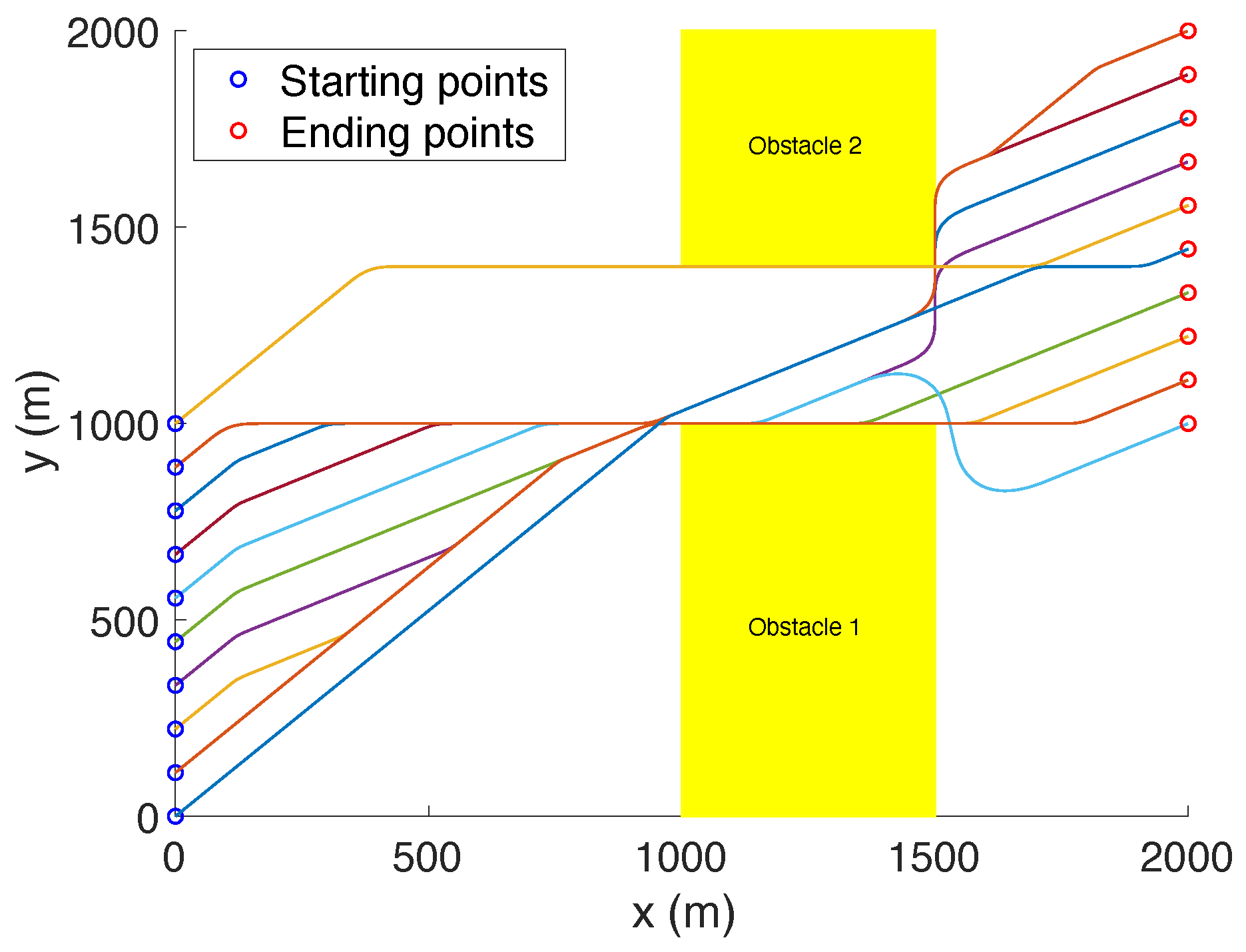
5.5. Test Case #5: Trajectory Planning for a Fleet of 13 UAVs

This scenario was chosen to compare the proposed algorithm with a visibility graph (VG)-based procedure with a similar anti-ollision technique not based on MIQP. The environment features eight obstacles located between the departure and target points. In the original study [9], the authors use a VG-based procedure to find the path for each UAV in the formation, which was proven to be optimal, so provides a good comparison to measure the solution quality loss in terms of path length that can occur using the proposed technique. However, the VG-based procedure considers Dubins’ arcs to smooth the piece-wise linear path, leading to discontinuities in the curvature, while the proposed algorithm uses clothoids, which better approximate aircraft behavior.

Table 8. Test case #5: main parameters and flight path optimization performance.

Scenario	VG + Dubins	Clothoids-Based
Number of UAVs	13	13
Minimum Turning Radius $R_{min}$ (m)	260	260
Number of Obstacles	12	12
Sum of UAV Path Lengths (km)	$410.22$	$416.39$

shows the main scenario parameters and results, comparing performance in terms of path length. To enable a direct comparison, the results obtained by the VG-based procedure were considered without the inclusion of the RVW points, which significantly reduce the required planning time. In terms of overall path length, the proposed procedure produced only 1.5% longer paths.

Figure 9 shows the obtained paths: most of the aircraft follow the same route between the first and second groups of obstacles, adopting a single-file formation to maintain separation distance. Only one aircraft chooses to pass the obstacles along a different path, remaining detached from the formation over the entire flight. This outcome highlights an aspect previously unaccounted for in the proposed procedure, namely, the management of a specific formation shape, which could become relevant in certain applications of flocking behavior.

6. Limitations and Discussion

Several numerical simulations were carried out, aimed at highlighting pros and cons of the proposed procedure with reference to: (1) ability to detect minimum-length trajectories in constrained/unconstrained environments, having fixed the departure and arrival points along with the respective directions; (2) ability to avoid collisions in case of multiple aircraft flying in formation. As for path planning capability, a comparison with a planning algorithm available in the literature based on randomly generated graphs showed that the proposed algorithm, by using a fixed environment decomposition, could to identify up to 10% shorter paths than the average one found by the random-based algorithm in almost all the tested grid configurations, although the latter could randomly find a better solution. Moreover, the use of clothoids in the proposed procedure has the advantage of making the resulting paths more compliant with aircraft dynamics by allowing a linear variation in curvature without discontinuities, unlike using a Dubins-based smoothing [9]. However, such an improvement comes at the cost of an overall increase in trajectory length (+1.5%), as demonstrated by the comparison with a procedure based on visibility graphs and Dubins curves.

Additionally, to properly define the clothoid curves, a graph based on predetermined directions is required, further limiting the optimality of the results. Nonetheless, despite these limitations, the proposed algorithm remains effective in planning both a single trajectory and trajectories of multiple aircraft, as proved by the results. From a collision avoidance capability point of view, as the algorithm neglects the management of the flight formation shape, it tends to consider overlapped pieces of trajectories, especially in the presence of narrow corridors limiting the passage of aircraft. To avoid any possible collision, a fast and effective method based on a single degree of freedom model was proposed, according to which aircraft can avoid collisions only by modifying their speed along the planned trajectory. Although it is an efficient and effective approach, there may be instances where speed constraints prevent finding a solution. In such cases, an exit strategy would be necessary to recalculate the trajectory, properly modifying some sections locally and avoiding some intersections. Furthermore, the current solution may limit the overall efficiency of the formation in terms of mission completion time due to the predetermined hierarchy, which the algorithm cannot overcome.

7. Conclusions

In this paper, a trajectory planning strategy for a fleet of UAVs was proposed. Initially, the trajectories of aircraft were developed as a sequence of piecewise linear paths smoothed through clothoid curves while optimizing the overall length using the shortest path algorithm within a graph. The use of clothoids was proved to be an effective way of creating flyable paths that can be easily followed by an automatic control system, representing a significant improvement over traditional straight-line or circular trajectories. Moreover, the collision avoidance problem between aircraft was dealt with by solving a mixed-integer optimal control problem, which optimizes the acceleration of each UAV of the flight formation along the planned trajectory.

The sensitivity analysis conducted on the proposed algorithm demonstrated that even with few routes and sparsely spaced grid points, the algorithm identifies flyable paths that comply with aircraft performance and environmental constraints. A comparison with another similar planning algorithm available in the literature showed that the use of fixed-points-/fixed-directions-based graphs allows the identification of better solutions than the average ones found by the random-based algorithm in almost all the tested grid configurations. Additionally, the use of an MIQP solver proveed its effectiveness as a collision avoidance technique even when multiple UAVs are flying together in a constrained environment.

The use of clothoids in the proposed procedure makes the trajectories more compliant with aircraft dynamics, although the overall length results slightly increased and the construction of the graph must be based on predetermined directions. Furthermore, the collision avoidance algorithm presents a limitation due to the need for a predetermined hierarchy between the aircraft, which could limit the overall efficiency of the formation in terms of mission completion time. These limitations form the basis of possible future developments of the algorithm, including the need to create an anticollision system capable of locally modifying trajectories to further optimize paths and properly manage formation shapes.

References

1. Federal Aviation Administration. FAA Aerospace Forecast. Fiscal Years 2022–2042; Federal Aviation Administration: Washington, DC, USA, 2022.
2. Ramesh, P.; Jeyan, J.M.L. Comparative analysis of the impact of operating parameters on military and civil applications of mini unmanned aerial vehicle (UAV). AIP Conf. Proc. 2020, 2311, 030034. [Google Scholar]
3. Aggarwal, S.; Kumar, N. Path planning techniques for unmanned aerial vehicles: A review, solutions, and challenges. Comput. Commun. 2020, 149, 270–299. [Google Scholar] [CrossRef]
4. Gul, F.; Mir, I.; Abualigah, L.; Sumari, P.; Forestiero, A. A consolidated review of path planning and optimization techniques: Technical perspectives and future directions. Electronics 2021, 10, 2250. [Google Scholar] [CrossRef]
5. Zhang, H.; Xin, B.; Dou, L.h.; Chen, J.; Hirota, K. A review of cooperative path planning of an unmanned aerial vehicle group. Front. Inf. Technol. Electron. Eng. 2020, 21, 1671–1694. [Google Scholar] [CrossRef]
6. Zhang, J.; Jiahao, X. Cooperative task assignment of multi-UAV system. Chin. J. Aeronaut. 2020, 33, 2825–2827. [Google Scholar] [CrossRef]
7. Beard, R.W.; McLain, T.W.; Goodrich, M.A.; Anderson, E.P. Coordinated target assignment and intercept for unmanned air vehicles. IEEE Trans. Robot. Autom. 2002, 18, 911–922. [Google Scholar] [CrossRef]
8. Qie, H.; Shi, D.; Shen, T.; Xu, X.; Li, Y.; Wang, L. Joint optimization of multi-UAV target assignment and path planning based on multi-agent reinforcement learning. IEEE Access 2019, 7, 146264–146272. [Google Scholar] [CrossRef]
9. D’Amato, E.; Mattei, M.; Notaro, I. Bi-level flight path planning of UAV formations with collision avoidance. J. Intell. Robot. Syst. 2019, 93, 193–211. [Google Scholar] [CrossRef]
10. Goerzen, C.; Kong, Z.; Mettler, B. A survey of motion planning algorithms from the perspective of autonomous UAV guidance. J. Intell. Robot. Syst. 2010, 57, 65. [Google Scholar] [CrossRef]
11. Souissi, O.; Benatitallah, R.; Duvivier, D.; Artiba, A.; Belanger, N.; Feyzeau, P. Path planning: A 2013 survey. In Proceedings of the 2013 International Conference on Industrial Engineering and Systems Management (IESM), Rabat, Morocco, 28–30 October 2013; IEEE: Piscataway, NJ, USA, 2013; pp. 1–8. [Google Scholar]
12. Radmanesh, M.; Kumar, M.; Guentert, P.H.; Sarim, M. Overview of path-planning and obstacle avoidance algorithms for UAVs: A comparative study. Unmanned Syst. 2018, 6, 95–118. [Google Scholar] [CrossRef]
13. Zhao, Y.; Zheng, Z.; Liu, Y. Survey on computational-intelligence-based UAV path planning. Knowl.-Based Syst. 2018, 158, 54–64. [Google Scholar] [CrossRef]
14. Dasgupta, B.; Gupta, A.; Singla, E. A variational approach to path planning for hyper-redundant manipulators. Robot. Auton. Syst. 2009, 57, 194–201. [Google Scholar] [CrossRef]
15. Shukla, A.; Singla, E.; Wahi, P.; Dasgupta, B. A direct variational method for planning monotonically optimal paths for redundant manipulators in constrained workspaces. Robot. Auton. Syst. 2013, 61, 209–220. [Google Scholar] [CrossRef]
16. Harada, M.; Nagata, H.; Simond, J.; Bollino, K. Optimal trajectory generation and tracking control of a single coaxial rotor UAV. In Proceedings of the AIAA Guidance, Navigation, and Control (GNC) Conference, Boston, MA, USA, 19–22 August 2013; p. 4531. [Google Scholar]
17. Xu, N.; Kang, W.; Cai, G.; Chen, B.M. Minimum-time trajectory planning for helicopter UAVs using computational dynamic optimization. In Proceedings of the Systems, Man, and Cybernetics (SMC), 2012 IEEE International Conference on, Seoul, Republic of Korea, 14–17 October 2012; IEEE: Piscataway, NJ, USA, 2012; pp. 2732–2737. [Google Scholar]
18. D’Amato, E.; Mattei, M.; Notaro, I. Distributed reactive model predictive control for collision avoidance of unmanned aerial vehicles in civil airspace. J. Intell. Robot. Syst. 2020, 97, 185–203. [Google Scholar] [CrossRef]
19. Scherer, S.; Singh, S.; Chamberlain, L.; Elgersma, M. Flying fast and low among obstacles: Methodology and experiments. Int. J. Robot. Res. 2008, 27, 549–574. [Google Scholar] [CrossRef]
20. Schøler, F.; la Cour-Harbo, A.; Bisgaard, M. Generating approximative minimum length paths in 3D for UAVs. In Proceedings of the Intelligent Vehicles Symposium (IV), 2012 IEEE, Madrid, Spain, 3–7 June 2012; IEEE: Piscataway, NJ, USA, 2012; pp. 229–233. [Google Scholar]
21. Maini, P.; Sujit, P.B. Path planning for a UAV with kinematic constraints in the presence of polygonal obstacles. In Proceedings of the Unmanned Aircraft Systems (ICUAS), 2016 International Conference on, Arlington, VA, USA, 7–10 June 2016; pp. 62–67. [Google Scholar]
22. Bortoff, S.A. Path planning for UAVs. Am. Control Conf. 2000, 1, 364–368. [Google Scholar]
23. Pehlivanoglu, Y.V. A new vibrational genetic algorithm enhanced with a Voronoi diagram for path planning of autonomous UAV. Aerosp. Sci. Technol. 2012, 16, 47–55. [Google Scholar] [CrossRef]
24. Lin, Y.; Saripalli, S. Path planning using 3D dubins curve for unmanned aerial vehicles. In Proceedings of the Unmanned Aircraft Systems (ICUAS), 2014 International Conference on, Orlando, FL, USA, 27–30 May 2014; IEEE: Piscataway, NJ, USA, 2014; pp. 296–304. [Google Scholar]
25. Véras, L.G.; Medeiros, F.L.; Guimarães, L.N. Rapidly exploring Random Tree* with a sampling method based on Sukharev grids and convex vertices of safety hulls of obstacles. Int. J. Adv. Robot. Syst. 2019, 16, 1729881419825941. [Google Scholar] [CrossRef]
26. Liu, Y.H.; Arimoto, S. Proposal of tangent graph and extended tangent graph for path planning of mobile robots. In Proceedings of the 1991 IEEE International Conference on Robotics and Automation, Sacramento, CA, USA, 9–11 April 1991; IEEE: Piscataway, NJ, USA, 1991; pp. 312–317. [Google Scholar]
27. Cover, H.; Choudhury, S.; Scherer, S.; Singh, S. Sparse tangential network (SPARTAN): Motion planning for micro aerial vehicles. In Proceedings of the 2013 IEEE International Conference on Robotics and Automation, Karlsruhe, Germany, 6–10 May 2013; IEEE: Piscataway, NJ, USA, 2013; pp. 2820–2825. [Google Scholar]
28. Babel, L. Curvature-constrained traveling salesman tours for aerial surveillance in scenarios with obstacles. Eur. J. Oper. Res. 2017, 262, 335–346. [Google Scholar] [CrossRef]
29. Musliman, I.A.; Rahman, A.A.; Coors, V. Implementing 3D network analysis in 3D GIS. Int. Arch. Isprs 2008, 37, 913–918. [Google Scholar]
30. De Filippis, L.; Guglieri, G.; Quagliotti, F. Path planning strategies for UAVS in 3D environments. J. Intell. Robot. Syst. 2012, 65, 247–264. [Google Scholar] [CrossRef]
31. Chang, B.R.; Tsai, H.F.; Lyu, J.L. Drone-Aided Path Planning for Unmanned Ground Vehicle Rapid Traversing Obstacle Area. Electronics 2022, 11, 1228. [Google Scholar] [CrossRef]
32. Carsten, J.; Ferguson, D.; Stentz, A. 3D field D: Improved path planning and replanning in three dimensions. In Proceedings of the 2006 IEEE/RSJ International Conference on Intelligent Robots and Systems, Beijing, China, 9–13 October 2006; IEEE: Piscataway, NJ, USA, 2006; pp. 3381–3386. [Google Scholar]
33. Liu, P.; Yu, H.; Cang, S. Geometric analysis-based trajectory planning and control for underactuated capsule systems with viscoelastic property. Trans. Inst. Meas. Control 2017, 40, 0142331217708833. [Google Scholar] [CrossRef]
34. Duan, H.; Zhao, J.; Deng, Y.; Shi, Y.; Ding, X. Dynamic Discrete Pigeon-Inspired Optimization for Multi-UAV Cooperative Search-Attack Mission Planning. IEEE Trans. Aerosp. Electron. Syst. 2021, 57, 706–720. [Google Scholar] [CrossRef]
35. Eun, Y.; Bang, H. Cooperative control of multiple unmanned aerial vehicles using the potential field theory. J. Aircr. 2006, 43, 1805–1814. [Google Scholar] [CrossRef]
36. Chen, X.; Zhang, J. The three-dimension path planning of UAV based on improved artificial potential field in dynamic environment. In Proceedings of the Intelligent Human-Machine Systems and Cybernetics (IHMSC), 2013 5th International Conference on, Hangzhou, China, 26–27 August 2013; IEEE: Piscataway, NJ, USA, 2013; Volume 2, pp. 144–147. [Google Scholar]
37. Kitamura, Y.; Tanaka, T.; Kishino, F.; Yachida, M. 3-D path planning in a dynamic environment using an octree and an artificial potential field. In Proceedings of the Intelligent Robots and Systems 95.’Human Robot Interaction and Cooperative Robots’, Proceedings. 1995 IEEE/RSJ International Conference on, Pittsburgh, PA, USA, 5–9 August 1995; IEEE: Piscataway, NJ, USA, 1995; Volume 2, pp. 474–481. [Google Scholar]
38. Roberge, V.; Tarbouchi, M.; Labonté, G. Fast Genetic Algorithm Path Planner for Fixed-Wing Military UAV Using GPU. IEEE Trans. Aerosp. Electron. Syst. 2018, 54, 2105–2117. [Google Scholar] [CrossRef]
39. Chai, R.; Tsourdos, A.; Savvaris, A.; Chai, S.; Xia, Y. Solving Constrained Trajectory Planning Problems Using Biased Particle Swarm Optimization. IEEE Trans. Aerosp. Electron. Syst. 2021, 57, 1685–1701. [Google Scholar] [CrossRef]
40. Belge, E.; Altan, A.; Hacıoğlu, R. Metaheuristic optimization-based path planning and tracking of quadcopter for payload hold-release mission. Electronics 2022, 11, 1208. [Google Scholar] [CrossRef]
41. Jia, Y.; Zhou, S.; Zeng, Q.; Li, C.; Chen, D.; Zhang, K.; Liu, L.; Chen, Z. The UAV Path Coverage Algorithm Based on the Greedy Strategy and Ant Colony Optimization. Electronics 2022, 11, 2667. [Google Scholar] [CrossRef]
42. Dever, C.; Mettler, B.; Feron, E.; Popovic, J.; McConley, M. Nonlinear trajectory generation for autonomous vehicles via parameterized maneuver classes. J. Guid. Control. Dyn. 2006, 29, 289–302. [Google Scholar] [CrossRef]
43. Frazzoli, E.; Dahleh, M.A.; Feron, E. Real-time motion planning for agile autonomous vehicles. Am. Control Conf. 2001, 1, 43–49. [Google Scholar]
44. Blasi, L.; Barbato, S.; D’Amato, E. A mixed probabilistic-geometric strategy for UAV optimum flight path identification based on bit-coded basic manoeuvres. Aerosp. Sci. Technol. 2017, 71, 1–11. [Google Scholar] [CrossRef]
45. Blake, W.; Multhopp, D. Design, performance and modeling considerations for close formation flight. In Proceedings of the 23rd Atmospheric Flight Mechanics Conference, Boston, MA, USA, 10–12 August 1998; p. 4343. [Google Scholar]
46. Chichka, D.F.; Speyer, J.L. Solar-powered, formation-enhanced aerial vehicle systems for sustained endurance. Am. Control Conf. 1998, 2, 684–688. [Google Scholar]
47. Proud, A.; Pachter, M.; D’Azzo, J. Close formation flight control. In Proceedings of the Guidance, Navigation, and Control Conference and Exhibit, Portland, OR, USA, 9–11 August 1999; p. 4207. [Google Scholar]
48. Pachter, M.; D’Azzo, J.J.; Proud, A.W. Tight formation flight control. J. Guid. Control. Dyn. 2001, 24, 246–254. [Google Scholar] [CrossRef]
49. Schumacher, C.; Singh, S. Nonlinear control of multiple UAVs in close-coupled formation flight. In Proceedings of the AIAA Guidance, Navigation, and Control Conference and Exhibit, Dever, CO, USA, 14–17 August 2000; p. 4373. [Google Scholar]
50. Mohiuddin, A.; Tarek, T.; Zweiri, Y.; Gan, D. A survey of single and multi-UAV aerial manipulation. Unmanned Syst. 2020, 8, 119–147. [Google Scholar] [CrossRef]
51. Skorobogatov, G.; Barrado, C.; Salamí, E. Multiple UAV systems: A survey. Unmanned Syst. 2020, 8, 149–169. [Google Scholar] [CrossRef]
52. Girard, A.R.; Howell, A.S.; Hedrick, J.K. Border patrol and surveillance missions using multiple unmanned air vehicles. In Proceedings of the 2004 43rd IEEE Conference on Decision and Control (CDC) (IEEE Cat. No. 04CH37601), Nassau, Bahamas, 14–17 December 2004; IEEE: Piscataway, NJ, USA, 2004; Volume 1, pp. 620–625. [Google Scholar]
53. Merino, L.; Caballero, F.; Martinez-de Dios, J.; Ollero, A. Cooperative fire detection using unmanned aerial vehicles. In Proceedings of the 2005 IEEE International Conference on Robotics and Automation, Barcelona, Spain, 18–22 April 2005; IEEE: Piscataway, NJ, USA, 2005; pp. 1884–1889. [Google Scholar]
54. Zengin, U.; Dogan, A. Real-time target tracking for autonomous UAVs in adversarial environments: A gradient search algorithm. IEEE Trans. Robot. 2007, 23, 294–307. [Google Scholar] [CrossRef]
55. Zhu, S.; Wang, D. Adversarial ground target tracking using UAVs with input constraints. J. Intell. Robot. Syst. 2012, 65, 521–532. [Google Scholar] [CrossRef]
56. Li, X.; Ci, L.; Yang, M.; Wei, H.; Tian, C.; Cheng, B. Multi-decision making based PSO optimization in airborne mobile sensor network deployment. In Proceedings of the 2012 IEEE 6th International Symposium on Embedded Multicore SoCs, Fukushima, Japan, 20–22 September 2012; IEEE: Piscataway, NJ, USA, 2012; pp. 128–134. [Google Scholar]
57. Sastry, S.; Meyer, G.; Tomlin, C.; Lygeros, J.; Godbole, D.; Pappas, G. Hybrid control in air traffic management systems. In Proceedings of the 1995 34th IEEE Conference on Decision and Control, New Orleans, LA, USA, 13–15 December 1995; IEEE: Piscataway, NJ, USA, 1995; Volume 2, pp. 1478–1483. [Google Scholar]
58. Bellingham, J.; Tillerson, M.; Richards, A.; How, J.P. Multi-task allocation and path planning for cooperating UAVs. In Cooperative Control: Models, Applications and Algorithms; Springer: Berlin/Heidelberg, Germany, 2003; pp. 23–41. [Google Scholar]
59. Yu, H.; Meier, K.; Argyle, M.; Beard, R.W. Cooperative path planning for target tracking in urban environments using unmanned air and ground vehicles. IEEE/ASME Trans. Mechatron. 2015, 20, 541–552. [Google Scholar] [CrossRef]
60. Shorakaei, H.; Vahdani, M.; Imani, B.; Gholami, A. Optimal cooperative path planning of unmanned aerial vehicles by a parallel genetic algorithm. Robotica 2016, 34, 823–836. [Google Scholar] [CrossRef]
61. Yao, P.; Wang, H.; Su, Z. Cooperative path planning with applications to target tracking and obstacle avoidance for multi-UAVs. Aerosp. Sci. Technol. 2016, 54, 10–22. [Google Scholar] [CrossRef]
62. Wu, J.; Yi, J.; Gao, L.; Li, X. Cooperative path planning of multiple UAVs based on PH curves and harmony search algorithm. In Proceedings of the Computer Supported Cooperative Work in Design (CSCWD), 2017 IEEE 21st International Conference on, Wellington, New Zealand, 26–28 April 2017; IEEE: Piscataway, NJ, USA, 2017; pp. 540–544. [Google Scholar]
63. Chandler, P.; Rasmussen, S.; Pachter, M. UAV cooperative path planning. In Proceedings of the AIAA Guidance, Navigation, and Control Conference and Exhibit, Dever, CO, USA, 14–17 August 2000; p. 4370. [Google Scholar]
64. Tsourdos, A.; White, B.; Shanmugavel, M. Cooperative Path Planning of Unmanned Aerial Vehicles; John Wiley & Sons: Hoboken, NJ, USA, 2010; Volume 32. [Google Scholar]
65. Lian, F.L.; Murray, R. Real-time trajectory generation for the cooperative path planning of multi-vehicle systems. In Proceedings of the Decision and Control, 2002, Proceedings of the 41st IEEE Conference on, Las Vegas, NV, USA, 10–13 December 2002; IEEE: Piscataway, NJ, USA, 2002; Volume 4, pp. 3766–3769. [Google Scholar]
66. Anderson, M.; Robbins, A. Formation flight as a cooperative game. In Proceedings of the Guidance, Navigation, and Control Conference and Exhibit, Boston, MA, USA, 10–12 August 1998; p. 4124. [Google Scholar]
67. Kuriki, Y.; Namerikawa, T. Consensus-based cooperative formation control with collision avoidance for a multi-UAV system. In Proceedings of the American Control Conference (ACC), Portland, OR, USA, 4–6 June 2014; IEEE: Piscataway, NJ, USA, 2014; pp. 2077–2082. [Google Scholar]
68. Ren, W.; Beard, R.W. Distributed Consensus in Multi-Vehicle Cooperative Control; Springer: Berlin/Heidelberg, Germany, 2008; Volume 27. [Google Scholar]
69. Ariola, M.; Mattei, M.; D’Amato, E.; Notaro, I.; Tartaglione, G. Model predictive control for a swarm of fixed wing uavs. In Proceedings of the 30Th Congress of the international council of the aeronautical sciences, Daejeon, Republic of Korea, 25–30 September 2016. [Google Scholar]
70. Blasi, L.; D’Amato, E.; Mattei, M.; Notaro, I. UAV Path Planning in 3D Constrained Environments Based on Layered Essential Visibility Graphs. IEEE Trans. Aerosp. Electron. Syst. 2022, 1–30. [Google Scholar] [CrossRef]
71. Al Nuaimi, M. Analysis and Comparison of Clothoid and Dubins Algorithms for UAV Trajectory Generation; West Virginia University: Morgantown, WY, USA, 2014. [Google Scholar]
72. Tuttle, T.; Wilhelm, J.P. Minimal length multi-segment clothoid return paths for vehicles with turn rate constraints. Front. Aerosp. Eng. 2022, 1. [Google Scholar] [CrossRef]
73. Bertolazzi, E.; Frego, M. Interpolating clothoid splines with curvature continuity. Math. Methods Appl. Sci. 2018, 41, 1723–1737. [Google Scholar] [CrossRef]
74. Meek, D.; Walton, D. Clothoid spline transition spirals. Math. Comput. 1992, 59, 117–133. [Google Scholar] [CrossRef]
75. Fraichard, T.; Scheuer, A. From Reeds and Shepp’s to continuous-curvature paths. IEEE Trans. Robot. 2004, 20, 1025–1035. [Google Scholar] [CrossRef]
76. Wilde, D.K. Computing clothoid segments for trajectory generation. In Proceedings of the 2009 IEEE/RSJ International Conference on Intelligent Robots and Systems, St Louis, MI, USA, 11–15 October 2009; IEEE: Piscataway, NJ, USA, 2009; pp. 2440–2445. [Google Scholar]
77. Gim, S.; Adouane, L.; Lee, S.; Derutin, J.P. Clothoids composition method for smooth path generation of car-like vehicle navigation. J. Intell. Robot. Syst. 2017, 88, 129–146. [Google Scholar] [CrossRef]
78. McLain, T.; Beard, R.W.; Owen, M. Implementing dubins airplane paths on fixed-wing uavs. In Handbook of Unmanned Aerial Vehicles; Springer: Dordrecht, The Netherlands, 2014. [Google Scholar]
79. Dubins, L.E. On curves of minimal length with a constraint on average curvature, and with prescribed initial and terminal positions and tangents. Am. J. Math. 1957, 79, 497–516. [Google Scholar] [CrossRef]
80. Dijkstra, E.W. A note on two problems in connexion with graphs. Numer. Math. 1959, 1, 269–271. [Google Scholar] [CrossRef]
81. Babel, L. Coordinated target assignment and UAV path planning with timing constraints. J. Intell. Robot. Syst. 2019, 94, 857–869. [Google Scholar] [CrossRef]
Figure 1. Intersection between the paths of the ith and jth UAV.
Electronics 12 02204 g001
Figure 2. Test case #1: Path planning considering several configuration parameters as shown in Table 2. (a) Minimum (rand min) and average (rand mean) path length found with the random-based graph compared with the minimum path length found with the fixed-based graph; (b) computational time, obtained with an Intel i5-8250u based laptop.
Electronics 12 02204 g002
Figure 3. Test case #1: Optimum paths with different grid configurations.
Electronics 12 02204 g003
Figure 4. Test case #2: Path planning considering several configuration parameters, as shown in Table 2. (a) Path length and (b) computational time, obtained with an Intel i5-8520u based laptop.
Electronics 12 02204 g004
Figure 5. Test case #2: Optimum paths with different grid configurations.
Electronics 12 02204 g005
Figure 6. Test case #3: Results. (a) Optimal fleet paths to avoid obstacles and reach target points; (b) UAVs mutual distances during flight.
Electronics 12 02204 g006
Figure 7. Test case #3: Planned optimal speeds (a) and accelerations (b) during flight to avoid collisions in path intersections.
Electronics 12 02204 g007
Figure 8. Test case #4: Optimal fleet paths to avoid obstacles and reach target points. Coloured lines show the planned trajectories for each UAV.
Electronics 12 02204 g008
Figure 9. Test case #5: Fleet optimal paths to avoid obstacles and reach target points.
Electronics 12 02204 g009