Capacity State-of-Health Estimation of Electric Vehicle Batteries Using Machine Learning and Impedance Measurements

Abstract

With the increasing adoption of electric vehicles (EVs) by the general public, a lot of research is being conducted in Li-ion battery-related topics, where state-of-health (SoH) estimation has a prominent role. Accurate knowledge of this parameter is essential for efficient and safe EV operation. In this work, machine-learning techniques are applied to estimate this parameter in EV applications and in diverse scenarios. After thoroughly analysing cell ageing in different storage conditions, a novel approach based on impedance data is developed for SoH estimation. A fully-connected feed-forward neural network (FC-FNN) is employed to estimate the battery’s maximum available capacity from a small set of impedance measurements. The method was tested for estimation in long-term scenarios and for diverse degradation procedures with data from real EV batteries. High accuracy was obtained in all situations, with a mean absolute error as low as 0.9%. Thus, the proposed algorithm constitutes a powerful and viable solution for fast and accurate SoH estimation in real-world battery management systems.

1. Introduction

The world’s mobility systems are experiencing a profound change as the market share of electric vehicles (EVs) increases for both personal and professional use. This has pushed forward the research on energy storage systems, where lithium-ion (Li-ion) batteries is the most widespread technology. Many different types of Li-ion chemistries exist depending on the choice of the positive and negative electrodes’ materials, each of them showing different characteristics. In EV applications, the most-common ones are lithium-nickel-manganese-cobalt (NMC) and lithium-nickel-cobalt-aluminium (NCA) [1].

In order to perform efficient energy and power control of an EV, as well as safe and reliable operation, an effective battery management system (BMS) must be implemented, which has state-of-health (SoH) estimation as one of its essential functions. This parameter is defined in this paper as the ratio of maximum available capacity at the current state to rated capacity, as in Equation (1).

$$SoH=\frac{Q_{max}}{Q_{rated}}*100$$

(1)

In recent years, many SoH estimation algorithms have been proposed based on different considerations. However, despite their great potential for solving complex modelling problems, a lot of possibilities for applying machine learning (ML) algorithms are yet to be explored.

1.1. State-of-the-Art Review

Over the last few years, plenty of SoH estimation algorithms have been proposed based on a wide variety of factors and procedures. A very comprehensive review of SoH estimation methods may be found in [2], considering both experimental and adaptive approaches, as well as some based on degradation-mechanism analysis. Another state-of-the-art review, but focused on just machine learning algorithms can be found in [3]. A detailed analysis of the procedures and results presented in these works shows that there is still room for improvement in terms of both applicability and performance, and that the correlation between impedance and maximum available capacity has not been exploited yet. Using impedance as health indicator has some interesting advantages over other methods: while approaches based on measurements taken while charging usually require a long time to complete, impedance can be measured in a very short time and without the need of charging the EV. This has been demonstrated by some recent works. In [4], the authors implemented two types of pseudo-random sequences, namely binary and ternary, to significantly reduce the execution time of the impedance measurements. A similar approach was applied in [5], but using the continuous Morse wavelet transform instead of the fast Fourier transform. Psuedo-random sequences were also employed in [6] with a focus on various implementation aspects in EV. Authors in [7] proposed using machine learning to reconstruct the entire impedance spectrum based on a few multi-sine signal injection measurements, which also reduced the execution time significantly. In [8], a very comprehensive analysis of battery ageing in different storage conditions was performed on long-term data. Then, a model was derived to predict the variation in some of the equivalent-circuit model parameters based on storage data. In [9], an SoH estimator was developed in the form of a support-vector regression algorithm which took as inputs the equivalent-resistance measurements at some specific state-of-charge levels.

1.2. Paper Contributions and Structure

In this paper, a new method for estimating EV batteries’ SoH is proposed by making use of machine learning and electrochemical impedance spectroscopy (EIS) data. The algorithm requires a very limited amount of impedance measurements at some fixed frequencies. This information is fed to a fully-connected feed-forward neural network (FC-FNN) to predict the cell’s maximum available capacity. Thus, the contributions of this paper are:

• Analysis of impedance measurements’ potential as health indicator to predict a battery’s maximum available capacity;
• Improved flexibility, since the execution constraints are relaxed, e.g., the algorithm does not require the battery to be charging;
• Highly-accurate estimations obtained with a limited number of measurements.

The remainder of the paper is organised as follows: the data set, the employed neural network and the estimation algorithm are described in Section 2. The experimental validation is outlined and the obtained results are presented in Section 3. Lastly, conclusions are drawn in Section 4.

The content of this paper is based on the work carried out by the corresponding author in relation to his master’s thesis [10] and built upon previous research of the same team [8,11].

2. Materials and Methods

2.1. Data Set Description

The data used throughout this work is composed of impedance and maximum capacity measurements taken from a set of BMW i3 battery modules, whose characteristics are presented in

Table 1. Characteristics of Li-ion cells used.

Chemistry	Nominal Capacity	Rated Voltage	Cut-Off Voltages
			Lower	Upper
NMC	63$\mathrm{A}$$\mathrm{h}$	$3.7$$\mathrm{V}$	3$\mathrm{V}$	$4.125$$\mathrm{V}$

. The former is obtained by means of electrochemical impedance spectroscopy, while the latter is found with constant-current, constant-voltage (CCCV) charge cycles.

Since in real-world EV applications batteries spend most of the time in an idle state, the ageing procedure employed for this research is focused on storage at different conditions in terms of state of charge (SoC) and temperature, as shown in

Table 2. Ageing conditions of Li-ion cells used.

Cell ID	C1	C2	C3	C4	C5	C6
SoC	50%	50%	50%	10%	90%	50%
Temperature	35 ${}^{°}\mathrm{C}$	40 ${}^{°}\mathrm{C}$	45 ${}^{°}\mathrm{C}$	45 ${}^{°}\mathrm{C}$	45 ${}^{°}\mathrm{C}$	7 ${}^{°}\mathrm{C}$

. This arrangement allows for a good study of the impact of both parameters on capacity loss while covering a wide range of realistic operation conditions of EV batteries.

The cells were taken out of storage once a month to conduct the reference performance tests. All experiments were performed at a constant temperature of 25 ${}^{°}\mathrm{C}$. Impedance was measured in galvanostatic mode at 10%, 50% and 90% SoC at 50 points from 10 $\mathrm{m}$$\mathrm{Hz}$ to 10 $\mathrm{k}$$\mathrm{Hz}$, while the charge and discharge C-rate was $0.2$ C. Data spanning around 13 months were recorded. A more comprehensive description of the data set and the experiments can be found in [8,11].

For simplicity purposes, only measurements corresponding to one of the SoC levels are employed for the degradation analysis and the development of the estimation algorithm. However, the impact of this factor on impedance must be assessed first. To that end, the measurements at all three charge levels are shown in Figure 1 for cell C1 at both pristine and aged stages.

The plot shows that cell’s SoC during the measurements does not have a significant impact on EIS results, specially when compared to ageing. Thus, this parameter can be neglected when developing the estimation algorithm, although it will be considered in the testing stage.

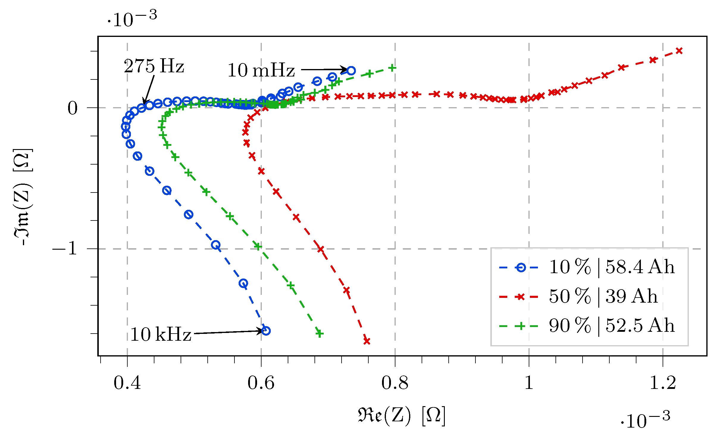
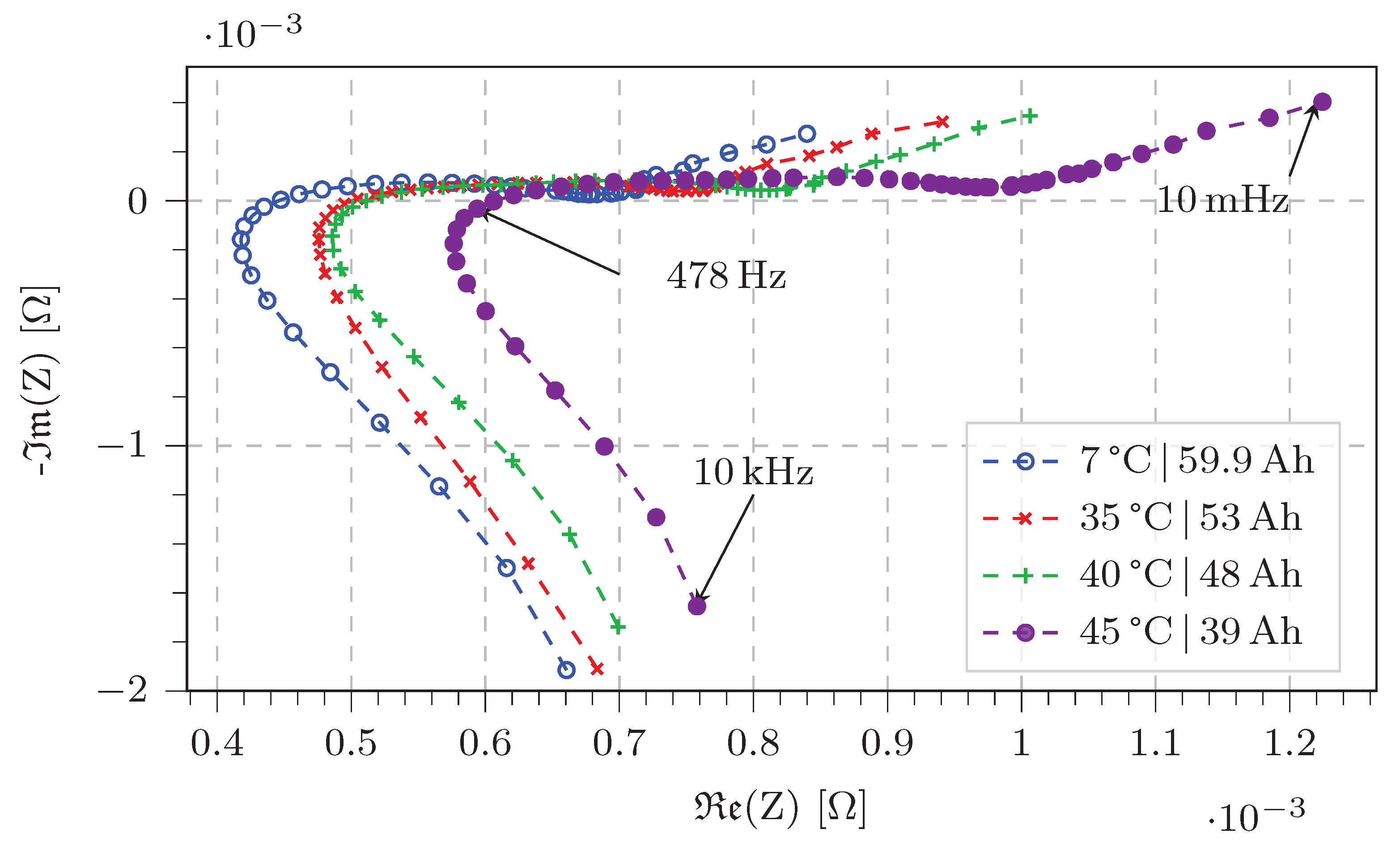
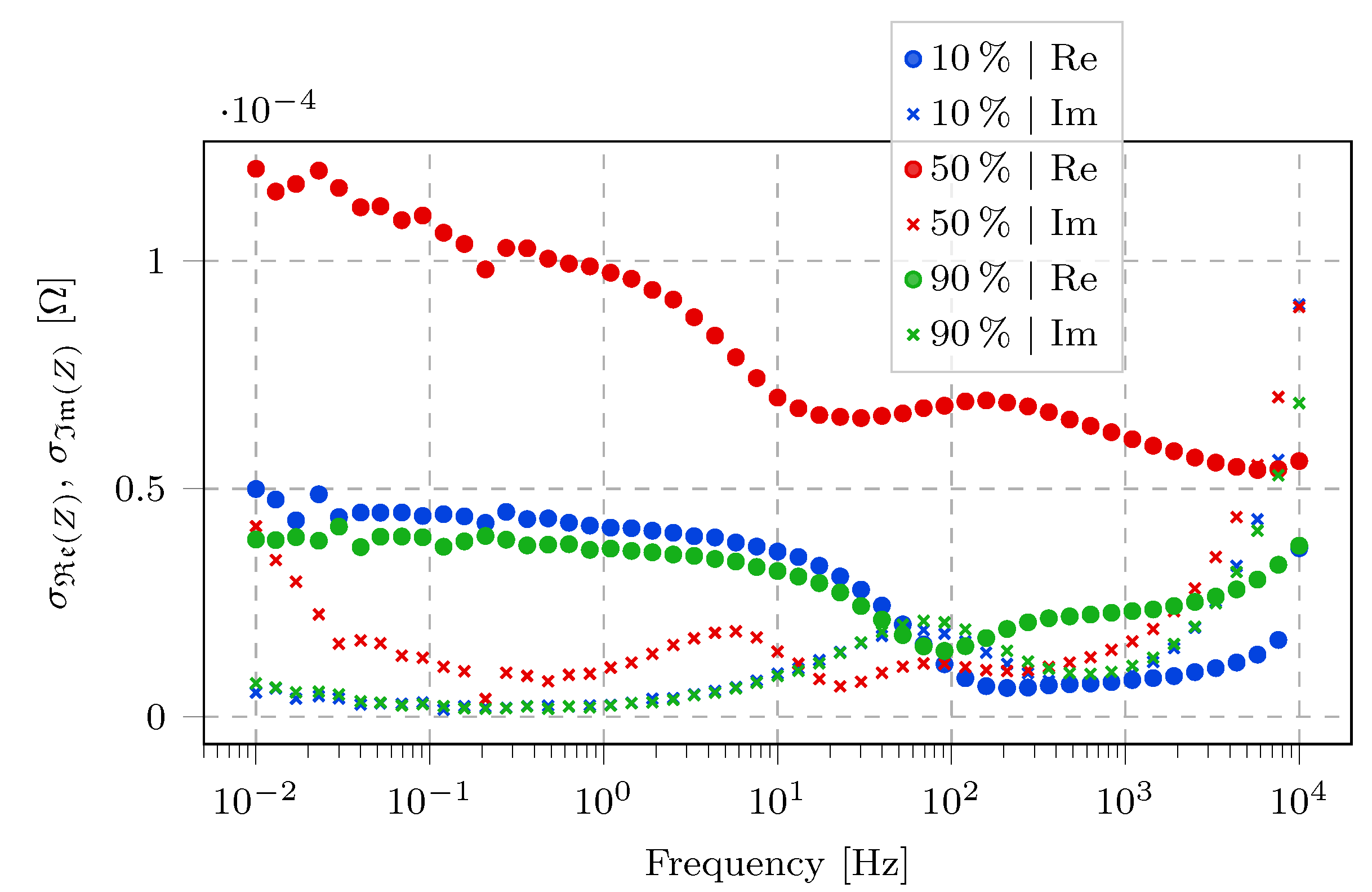
2.2. Degradation Analysis

In order to analyse the relationship between maximum available capacity and cell impedance, the evolution of cell C1’s impedance as the experiment progressed is depicted in the Nyquist plot in Figure 2 and the Bode plot in Figure 3. The connection between these two diagrams is that points in the upper-right zone of the Nyquist plot correspond to low-frequency measurements, while those in the lower-left area are from high-frequency ones.

In the Nyquist plot, a clear tendency of increasing real part with degradation can be observed, which occurs at all frequencies. The same behaviour can be noted from the Bode plot, which shows how the impedance’s magnitude becomes larger with degradation, while its phase experiences a similar variation. The main consequence of this impedance increment would be higher losses when charging and discharging the battery and, thus, lower energy efficiency. This correlation between degradation and cell impedance is the fundamental argument for using these measurements as health indicators.

Based on the collected data, it is possible to analyse how cells stored at different temperatures and SoC levels deteriorate. Figure 4 shows the evolution of the cells’ maximum available capacity as time passed. When looking at data from cells aged at the same SoC level $\left(50\%\right)$, capacity loss is largest at the hottest temperature $\left(45 {}^{°}\mathrm{C}\right)$ and lowest at the coldest one $\left(7 {}^{°}\mathrm{C}\right)$. At the same time, when comparing between similar storage temperatures $\left(45 {}^{°}\mathrm{C}\right)$, degradation was most significant for cells which where halfway charged $\left(50\%\right)$ than for those closer to maximum $\left(90\%\right)$ and minimum $\left(10\%\right)$ levels, being the latter the one with lowest capacity decay. It can also be observed how there exists a considerable difference between the best and worst cases, which retained $59.8$ $\mathrm{A}$$\mathrm{h}$ and $38.9$ $\mathrm{A}$$\mathrm{h}$ after 13 months in storage. In terms of SoH, these correspond to 98% and 63.8%, respectively.

Figure 5 shows the Nyquist plot of cells which were stored at the same temperature $\left(45 {}^{°}\mathrm{C}\right)$ and three different SoC levels $\left(10\%,50\%\mathrm{and}90\%\right)$. Data corresponds to measurements at 50% SoC after 13 months in storage. It can be observed how resistance increment is much more significant for cells stored at intermediate charge levels than for the ones which were almost depleted or full. Between the extremes, capacity loss was lower when the battery was stored at lower SoC.

Similarly, Figure 6 shows the Nyquist plot of cells which were aged at the same SoC $\left(50\%\right)$ and multiple temperatures $\left(7 {}^{°}\mathrm{C},35 {}^{°}\mathrm{C},40 {}^{°}\mathrm{C}\mathrm{and}45 {}^{°}\mathrm{C}\right)$. In this case, impedance evolution becomes more severe for those cells which were kept at hotter temperatures than for those stored at colder temperatures.

These plots prove that storage conditions play a major role in a battery’s capacity and impedance degradation, being cold temperatures and extreme charge levels the most beneficial ones. Furthermore, they also show that, in general, capacity loss is linked to an increase in the impedance’s real part at all frequencies or, in other words, a rightwards displacement of the Nyquist plots. This evolution will be exploited when designing the SoH estimation algorithm.

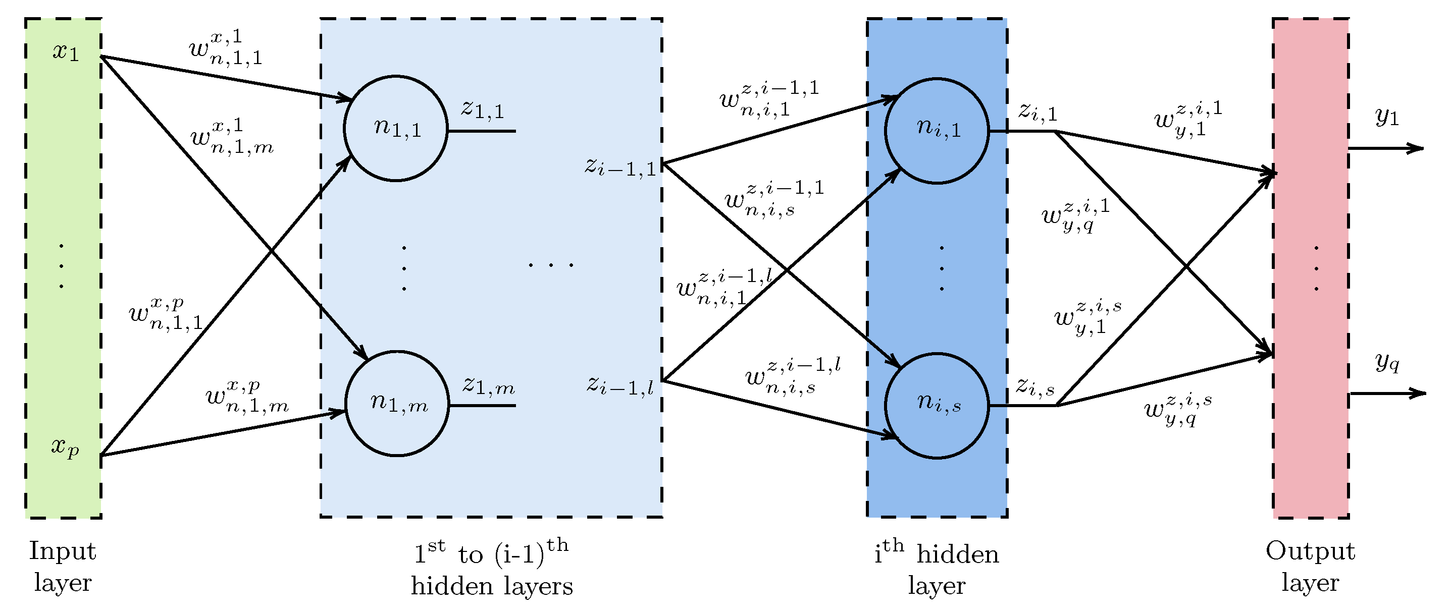
2.3. Fully-Connected Feed-Forward Neural Networks

For this work, a very simple fully-connected feed-forward neural network is chosen as an estimator. Although not the most powerful ML structure, FC-FNNs provide a good trade-off between accuracy, simplicity and low computational cost. This is due to the fact that, as will be shown throughout this section, they consist of simple linear operations (additions and multiplications) which can be carried out swiftly even in low-power processors. Furthermore, these can be parallelized to make the algorithm even more efficient. They are made up of several layers stacked one after another, each of them containing several individual neurons. Every neuron takes as inputs the outputs of all the neurons in the previous layer, which are multiplied by the corresponding weights and added to the bias term. Lastly, a non-linear activation function is applied to the result, such as the hyperbolic tangent or the rectified linear unit (ReLU). The operation carried out in each neuron is given by Equation (2), where $f\left(\alpha \right)$ is the non-linear activation function. A general diagram of the FC-FNN is shown in Figure 7, with the symbols as defined in

Table 3. Description of symbols of FC-FNN in Figure 7.

Symbol	Description
$\mathit{x}=\left[x_1,\cdots ,x_p\right]$	Input data vector
$\mathit{y}=\left[y_1,\cdots ,y_q\right]$	Output data vector
$w_{n,1,m}^{x,p}$	Weight from input $x_p$ to mth neuron in 1st hidden layer
$w_{n,i,s}^{z,i-1,l}$	Weight from lth neuron in $\left(i-1\right)$th hidden layer to sth neuron in ith hidden layer
$w_{y,q}^{z,i,s}$	Weight from sth neuron in ith hidden layer to output $y_q$

.

$$y=f\left(\alpha \right)=f\left(\sum _{i=1}^n{w}_i{x}_i+b\right)=f\left(\mathit{w}{\mathit{x}}^T+b\right)$$

(2)

The weights in the network are updated following the back-propagation algorithm with stochastic gradient descent. An Adam optimiser is used with mean-squared-error (MSE) as loss metric, along with early stopping and batch training to avoid over-fitting while training. The data split between training and validation is 70% and 30% of the samples, respectively.

For the remainder of the paper, the nomenclature used for describing the FC-FNN structure will be $FNN\left(n_1-\dots -n_i,AF\right)$, where $n_1$ is the number of neurons in the first hidden layer, $n_i$ is the amount of neurons in the last one and AF denotes the activation function employed in all neurons.

2.4. Impedance-Based SoH Estimation Algorithm

The method proposed in this paper aims at predicting a cell’s maximum available capacity based on a very limited set of impedance measurements. The choice of which frequencies to use is critical in order to guarantee good performance and applicability. Two criteria are fundamentally used for this purpose: first, large differences should exist between a pristine and an aged cell in terms of complex impedance value. Secondly, intermediate frequencies are preferred over extreme ones, since low-frequency measurements would greatly increase the process’ duration, and high-frequency ones could lead to larger errors caused by the inductive behaviour of the wiring. It is also desired to keep the amount of points to a minimum so that the entire estimation process can be performed faster.

The variation of impedance throughout ageing can be easily quantified by computing the standard deviation of the impedance at each frequency for the entire experiment’s period. Thus, high values of standard deviation would indicate that differences are larger at that given frequency and, therefore, that the point is more relevant as health indicator. Figure 8 shows this metric for cells aged at the same temperature $\left(45 {}^{°}\mathrm{C}\right)$, while Figure 9 does so for cells stored at the same SoC level $\left(50\%\right)$.

It is clear that relevant differences exist only in the real part of the impedance, since the imaginary part’s standard deviation is quite low, no matter the ageing procedure. Thus, the largest variations correspond to the cell stored at 50% SoC when considering same-temperature experiments, while they are highest for the cell kept at 45 ${}^{°}\mathrm{C}$ in same-SoC ones. This is consistent with the previous degradation analysis, since these were the cells who experienced the largest capacity loss (see Figure 4) and the largest impedance change (see Figure 5 and Figure 6) by the end of the experiment. Figure 8 and Figure 9 also show that, as expected from Figure 5 and Figure 6, impedance variation is not the same at all frequencies and, thus, some points are more relevant that others to exploit the phenomenon described throughout this paper.

Based on these considerations it was chosen to use the following frequencies as feature points: 10 $\mathrm{Hz}$, 20 $\mathrm{Hz}$, 50 $\mathrm{Hz}$, 100 $\mathrm{Hz}$, 200 $\mathrm{Hz}$, 500 $\mathrm{Hz}$ and 1 $\mathrm{k}$$\mathrm{Hz}$. The input vector to the FC-FNN is then built following Equation (3), while the output is the cell’s estimated maximum available capacity $\left({\widehat{Q}}_{max}\right)$.

$$\begin{array}{cc}\hfill \mathit{x}=& [\mathrm{Re}\left(Z_{10}\right),\mathrm{Re}\left(Z_{20}\right),\mathrm{Re}\left(Z_{50}\right),\mathrm{Re}\left(Z_{100}\right),\mathrm{Re}\left(Z_{200}\right),\mathrm{Re}\left(Z_{500}\right),\mathrm{Re}\left(Z_{1000}\right),\hfill \\ \hfill & \mathrm{Im}\left(Z_{10}\right),\mathrm{Im}\left(Z_{20}\right),\mathrm{Im}\left(Z_{50}\right),\mathrm{Im}\left(Z_{100}\right),\mathrm{Im}\left(Z_{200}\right),\mathrm{Im}\left(Z_{500}\right),\mathrm{Im}\left(Z_{1000}\right){]}^T\hfill \end{array}$$

(3)

It must be noted that these are approximated frequency values, since they do not perfectly match the ones present in the data set. Exactness is not a critical aspect in the proposed approach, as long as the frequencies used in the real application are the same ones as during training.

3. Results

In order to evaluate the performance of the proposed algorithm, two different scenarios are designed: in the first one, the FC-FNN is trained with all the data from a set of cells (C1, C2, C3, C4) and then tested on data from units aged in different conditions (C5, C6). Secondly, the algorithm is trained with only a part of the entire time series (0–10 months) and then tested on the remaining part (11–13 months). The former aims at verifying if recording data in a limited set of conditions is enough to make predictions no matter the ageing procedure, while the latter assesses the accuracy of the algorithm when facing deeper-degradation data. Additionally, to further investigate the applicability of the method, all three available SoC levels are tested.

The performance metrics used are the root mean squared error ($RMSE$), the mean absolute error ($MAE$) and the maximum absolute error ($ME$), as well as the residuals’ mean (${\mu }_{\mathrm{res}}$) and standard deviation (${\sigma }_{\mathrm{res}}$), all of them normalized. The formulas for these metrics are as given by Equations (4) and (5), where ${\widehat{y}}_i,y_i$ are the estimated and real output values of the ${\mathrm{i}}^{\mathrm{th}}$ sample, respectively, and N is the total number of samples.

$$\begin{array}{cccccc}\hfill e_i& =\frac{{\widehat{y}}_i-y_i}{y_i}\hfill & \hfill {\mu }_{res}& =\frac{1}{N}\sum _{i=0}^{N-1}{e}_i\hfill & \hfill {\sigma }_{res}& =\sqrt{\frac{1}{N}\sum _{i=0}^{N-1}{\left(e_i-{\mu }_{res}\right)}^2}\hfill \end{array}$$

(4)

$$\begin{array}{cccccc}\hfill RMSE& =\sqrt{\frac{1}{N}\sum _{i=0}^{N-1}{e}_i^2}\hfill & \hfill MAE& =\frac{1}{N}\sum _{i=0}^{N-1}\left|e_i\right|\hfill & \hfill ME& =max\left(\left|e_i\right|\right)\hfill \end{array}$$

(5)

Besides the error rates, the amount of weights in each of the networks is given to provide some insight on the computational requirements of each of the models. These, added with the total amount of neurons in each network, define the memory usage.

3.1. SoC-Dependent Capacity Estimation

In this case, an independent estimator, i.e., a different FC-FNN, is trained and tested for each SoC level. The obtained results are presented in

Table 4. Test results with impedance measurements at 10% SoC.

Train	Test	Structure	RMSE	MAE	ME	${\mathsf{\mu }}_{\mathbf{res}}$	${\mathsf{\sigma }}_{\mathbf{res}}$
C1–C4 0–13 M	C5–C6 0–13 M	FNN (10-10-10, ReLU)	2.8%	1.7%	10%	−1.5%	2.3%
C1–C6 0–10 M	C1–C6 11–13 M	FNN (10-10-10, ReLU)	2.4%	1.7%	5.4%	1.7%	1.2%

,

Table 5. Test results with impedance measurements at 50% SoC.

Train	Test	Structure	RMSE	MAE	ME	${\mathsf{\mu }}_{\mathbf{res}}$	${\mathsf{\sigma }}_{\mathbf{res}}$
C1–C4 0–13 M	C5–C6 0–13 M	FNN (10-10-10, ReLU)	2%	1.4%	5.9%	0%	2%
C1–C6 0–10 M	C1–C6 11–13 M	FNN (10-10-10, ReLU)	2.1%	1.6%	5.8%	1.6%	1.5%

and

Table 6. Test results with impedance measurements at 90% SoC.

Train	Test	Structure	RMSE	MAE	ME	${\mathsf{\mu }}_{\mathbf{res}}$	${\mathsf{\sigma }}_{\mathbf{res}}$
C1–C4 0–13 M	C5–C6 0–13 M	FNN (10-10-10, ReLU)	1.5%	0.9%	6.3%	−0.2%	1.5%
C1–C6 0–10 M	C1–C6 11–13 M	FNN (10-10-10, ReLU)	2.5%	1.9%	6%	1.8%	1.9%

for 10%, 50% and 90% SoC, respectively.

It can be observed that the algorithm performs very well in all cases, with similar error rates in both scenarios. The algorithm could be made even more accurate if more data were available or by adding more neurons and layers. It was chosen not to do so to keep the amount of parameters as low as possible.

3.2. SoC-Independent Capacity Estimation

In order to further test the proposed approach’s capabilities, a final test is conducted in which data from all three available SoC levels are merged into a single data set, while keeping the input vector as defined in Equation (3). The same two scenarios as before are used. The goal is to verify whether the algorithm can work properly no matter the current SoC of the battery, since this parameter was shown to have little effect on impedance (see Section 2.1). Results are presented in

Table 7. Test results with combined impedance measurements.

Train	Test	Structure	RMSE	MAE	ME	${\mathsf{\mu }}_{\mathbf{res}}$	${\mathsf{\sigma }}_{\mathbf{res}}$
C1–C4 0–13 M	C5–C6 0–13 M	FNN (10-10-10, ReLU)	1.9%	1.1%	6.3%	−0.2%	2.1%
C1–C6 0–10 M	C1–C6 11–13 M	FNN (10-10-10, ReLU)	3.1%	2.7%	5%	2.5%	1.8%

.

This shows that, even though the algorithm also works well when the influence of the SoC in impedance is neglected, accuracy is sensibly lower than in the SoC-dependent test cases.

4. Conclusions

The proposed algorithm showed great performance on challenging scenarios, combining very low estimation errors with low computational cost, since only seven complex impedance measurements and a very compact model were required. Despite these very good results, the low amount of recorded data definitely had a negative impact on performance.

It has been shown that a relationship between impedance spectrum and maximum available capacity exists and can thus be exploited for SoH estimation. The use of ML algorithms simplified the modelling of such relationship, as these do not require comprehensive electrochemical knowledge of the inner operation principles of the battery. The method developed in this work showed very good accuracy with an MAE below 2% when facing new data from different ageing procedures, as well as when making long-term predictions. The proposed approach greatly improves applicability, since impedance measurements may be conducted at any time as soon as the battery is at some specific SoC level and temperature, which reduces to only temperature if the combined method is used. For future works, more degradation data need to be collected from more batteries and conditions in order to enhance and evaluate performance even further.

References

1. Miao, Y.; Hynan, P.; von Jouanne, A.; Yokochi, A. Current Li-ion Battery Technologies in Electric Vehicles and Opportunities for Advancements. Energies 2019, 12, 1074. [Google Scholar] [CrossRef] [Green Version]
2. Berecibar, M.; Gandiaga, I.; Villarreal, I.; Omar, N.; Van Mierlo, J.; Van den Bossche, P. Critical Review of State of Health Estimation Methods of Li-ion Batteries for Real Applications. Renew. Sustain. Energy Rev. 2016, 56, 572–587. [Google Scholar] [CrossRef]
3. Vidal, C.; Malysz, P.; Kollmeyer, P.; Emadi, A. Machine Learning Applied to Electrified Vehicle Battery State of Charge and State of Health Estimation: State-of-the-Art. IEEE Access 2020, 8,, 52796–52814. [Google Scholar] [CrossRef]
4. Sihvo, J.; Stroe, D.; Messo, T.; Roinila, T. Fast Approach for Battery Impedance Identification Using Pseudo-Random Sequence Signals. IEEE Trans. Power Electron. 2020, 35, 2548–2557. [Google Scholar] [CrossRef]
5. Nusev, G.; Juričić, D.; Gaberšček, M.; Moškon, J.; Boškoski, P. Fast Impedance Measurement of Li-ion Battery Using Discrete Random Binary Excitation and Wavelet Transform. IEEE Access 2021, 9, 46152–46165. [Google Scholar] [CrossRef]
6. Geng, Z.; Thiringer, T.; Olofsson, Y.; Groot, J.; West, M. On-board Impedance Diagnostics Method of Li-ion Traction Batteries Using Pseudo-Random Binary Sequences. In Proceedings of the 2018 20th European Conference on Power Electronics and Applications (EPE’18 ECCE Europe), Riga, Latvia, 17–21 September 2018; pp. 1–9. [Google Scholar]
7. Chen, C.; Yesilbas, G.; Lenz, A.; Schneider, O.; Knoll, A.C. Machine Learning Approach for Full Impedance Spectrum Study of Li-ion Battery. In Proceedings of the 46th Annual Conference of the IEEE Industrial Electronics Society (IECON), Singapore, 18–21 October 2020; pp. 3747–3752. [Google Scholar]
8. Gismero, A.; Stroe, D.-I.; Schaltz, E. Calendar Ageing Lifetime Model of NMC-based Lithium-ion Batteries Based on EIS Measurements. In Proceedings of the 2019 Fourteenth International Conference on Ecological Vehicles and Renewable Energies (EVER), Monte-Carlo, Monaco, 8–10 May 2019. [Google Scholar]
9. Tan, X.; Tan, Y.; Zhan, D.; Yu, Z.; Fan, Y.; Qiu, J.; Li, J. Real-time State-of-Health Estimation of Lithium-ion Batteries Based on the Equivalent Internal Resistance. IEEE Access 2020, 8, 56811–56822. [Google Scholar] [CrossRef]
10. <b>Barragán-Moreno, A. Machine Learning-based Online State-of-Health Estimation of Electric Vehicle Batteries. Master’s Thesis, Aalborg Universitet (AAU), Aalborg, Denmark, 14 June 2021. [Google Scholar]
11. Schaltz, E.; Stroe, D.-I.; Nørregaard, K.; Stenhøj Kofod, L.; Christensen, A. Incremental Capacity Analysis Applied on Electric Vehicles for Battery State-of-Health Estimation. IEEE Trans. Ind. Appl. 2021, 57, 1810–1817. [Google Scholar] [CrossRef]
Figure 1. Nyquist plot of cell C1’s impedance at beginning of life and after 13 months. Measurements performed at 25 ° C and 3 SoC levels. In the legend, left column represents SoC when impedance was measured, while right one is the measured maximum available capacity.
Electronics 11 01414 g001
Figure 2. Nyquist plot of cell C1’s impedance with ageing. Measurements taken at 50% SoC and 25 ° C . Legend shows the measured maximum available capacity.
Electronics 11 01414 g002
Figure 3. Bode plot of cell C1’s impedance with ageing. Measurements performed at 50% SoC and 25 ° C . Legend shows the measured maximum available capacity. For clarity purposes, only the segment with most significant differences is shown.
Electronics 11 01414 g003
Figure 4. Capacity degradation for different storage conditions. Measurements taken at 25 ° C . In the legend, the leftmost column represents the storage SoC, and the rightmost one, the storage temperature.
Electronics 11 01414 g004
Figure 5. Nyquist plot of impedance of cells stored at the same temperature 45   ° C after 13 months. Measurements performed at 50% SoC and 25 ° C . In the legend, the leftmost column represents storage SoC, and the rightmost column shows the maximum available capacity.
Electronics 11 01414 g005
Figure 6. Nyquist plot of impedance of cells stored at the same SoC 50 % after 13 months. Measurements performed at 50% SoC and 25 ° C . In the legend, the leftmost column represents storage temperature, and the rightmost column shows the maximum available capacity.
Electronics 11 01414 g006
Figure 7. Diagram of fully-connected feed-forward neural network.
Electronics 11 01414 g007
Figure 8. Impedance’s standard deviation in different storage SoC and same temperature 45   ° C conditions. Legend shows the storage SoC.
Electronics 11 01414 g008
Figure 9. Impedance’s standard deviation in different storage temperature and same SoC 50 % conditions. Legend shows the storage temperature.
Electronics 11 01414 g009