Finite-Time Neural Network Fault-Tolerant Control for Robotic Manipulators under Multiple Constraints

Abstract

In this study, a backstepping-based fault-tolerant controller for a robotic manipulator system with input and output constraints was developed. First, a barrier Lyapunov function was adopted to ensure that the system output satisfied time-varying constraints. Subsequently, the actuator input saturation and asymmetric dead-zone characteristics were also considered, and the actuator characteristics were described using a continuous function. The impacts of actuator failures and unknown dynamical parameters of the system were eliminated by employing Gaussian radial basis function neural networks. The external disturbances were compensated for, using a disturbance observer. Meanwhile, a finite-time dynamic surface technique was adopted to accelerate the convergence of the system errors. Finally, simulation of a 2-degrees-of-freedom robotic manipulator system showed the effectiveness of the proposed controller.

1. Introduction

Practical applications, such as robotic, electrical, and hydraulic systems, are frequently subject to input and output constraints, owing to their intrinsic characteristics. For instance, saturation, dead zone, hysteresis, and other input constraints have a direct impact on the response of the actuator [1,2,3,4,5,6], which affects system output performance. Meanwhile, the output or state constraints must be considered during the system controller design process to satisfy the system output performance criteria. However, these constraints do not exist individually. If these multi-constraint problems are disregarded during the design process, the system performance may deteriorate or fail. Thus, it is necessary to eliminate the influence of these nonlinear characteristics.

In recent years, numerous strategies to ensure the stability and performance of a system with dead-zone characteristics have been proposed [1,7,8,9,10,11,12,13,14,15,16,17,18]. For instance, to eliminate the influence of the dead-zone characteristic, in [7,8] an effective control was achieved by constructing a dead-zone inverse function, and the dead-zone characteristic was described by a linear function in [9,10]. An optimization algorithm was adopted in [19], where the authors treated the input dead-zone characteristic as a bounded function and adopted an adaptive approach to overcome the nonlinear characteristics. An adaptive fuzzy controller was utilized to compensate for the dead zone in [20], both of which avoided the problem of constructing the dead-zone inverse. With the development of neural networks (NNs) technology, in [21], for a flexible robotic arm system, the NNs approach was conquered based on the effect of dead-zone characteristics. In addition, owing to the performance requirements of the system, its output is subject to certain constraints [22,23,24,25]; the barrier Lyapunov function (BLF) is a common method for dealing with output or state constraint problems. In [26], a logarithmic BLF was applied to the control-law design of a robot. The control problem of a robotic arm system with time-varying output constraints was studied in [27], and an effective controller was presented for the model of a marine vessel under asymmetric constraints in [28], both of which expanded the application scenarios of the BLF. However, only a single constraint was considered in the aforementioned works, and the constraints appeared in multiple forms in practical application scenarios. Therefore, the control law design under multiple constraints is worth investigating.

Furthermore, as the working time and environment change, the actuators in the system are prone to failure, which has an adverse impact on the system performance. Numerous successful outcomes have recently been demonstrated in terms of addressing the control challenges caused by actuator faults [29,30,31,32,33,34,35,36,37,38,39,40]. For instance, the effects of actuator failures and disturbances were handled using an adaptive-based strategy in [31] and eliminated using the NNs technique in [33]. Based on the backstepping strategy, the switched system overcame the effects of faults and achieved a fast convergence of errors in [34]. In [35,36], reasonable control laws were devised for the flexible robotic and spacecraft systems, respectively, and the system remained stable in the event of actuator failure without violating the constraints. In [37], an effective controller was designed to eliminate the effect of actuator failure by combining fuzzy and backstepping controls. However, in the aforementioned types of fault-tolerant control, the control problem under multiple constraints is rarely considered, and the combination of multiple constraints and actuator faults makes the controller design more challenging, thereby inspiring our research.

Inspired by the previous work, in this paper, based on the NNs and dynamic surface control (DSC) approach, we develop a suitable controller for a robotic system with multiple constraints and actuator failures. Compared with the existing work, the main contributions are as follows:

• Compared to the results in [1,10,31,33,36], this study considered actuators with multiple constraints. The hyperbolic tangent function and asymmetric dead-zone function were introduced to describe the input characteristics of the system. The entire design process was based on the backstepping scheme in which the DSC and Nussbaum functions are utilized to optimize the design process.
• In contrast to [11,33], time-varying output constraints were considered to ensure that the system still met the performance requirements, even if actuator failure occurred. The NNs approach was utilized to fit the unknown parameters and faults of the robots.
• Based on [11], a finite-time filter was applied to optimize the design process and achieve fast convergence of the system error.

2. Problem Formulation

In this paper, we will study the problem of fault-tolerant control of a manipulator system with multiple constraints. The constraints considered include input saturation, dead zone, and time-varying output constraints.

Considering the uncertainty of the system structure and the possible actuator failures during operation, we employ radial basis function neural networks to compensate for the unknown continuous functions:

$$\begin{array}{c}{f}_i\left(Z\right):{\mathbb{R}}^q\to \mathbb{R}\hfill \\ f_i\left(Z\right)=W_i^T{S}_i\left(Z\right), i=1,2,\dots ,n\hfill \end{array}$$

(1)

where $W_{}={[W_1,W_2,\dots ,W_l]}^T\in {\mathbb{R}}^l$ is the weight vector, and l is the number of nodes in the hidden layer of the NNs. Theoretically, when l is chosen to be large enough, the output $W_i^T{S}_i\left(Z\right)$ of NNs can achieve an exact approximation for any continuous function. $Z={[Z_1,Z_2,\dots ,Z_q]}^T\in {\mathrm{\Omega }}_N\subset {\mathbb{R}}^q$ is the NNs input vector, and $S_i={[s_1,s_2,\dots ,s_l]}^T\in {\mathbb{R}}^l$ is the output value of the activation function. The approximation process of the NNs is described as

$$\begin{array}{cc}\hfill f_i\left(Z\right)=& W_i^{*T}{S}_i\left(Z\right)+{\epsilon }_i\left(Z\right) \forall Z\in {\mathrm{\Omega }}_N\subset {\mathbb{R}}^q\hfill \\ \hfill & i=1,2,\dots ,n\hfill \end{array}$$

(2)

where $W^{*}={[W_1^{*},W_2^{*},\dots ,W_l^{*}]}^T$ is the vector of ideal weights, and ${\epsilon }_i={[{\epsilon }_1,{\epsilon }_2,\dots ,{\epsilon }_l]}^T$ is the approximation error that satisfies $\left|{\epsilon }_i\left(Z\right)\right|\le {\overline{\epsilon }}_i$, where ${\overline{\epsilon }}_i>0$ is an unknown bound. The Gaussian-type activation function is

$$s_k\left(Z\right)=exp\left[\frac{-{\left(Z-{\mu }_k\right)}^T\left(Z-{\mu }_k\right)}{{\eta }_k^2}\right],k=1,2,\dots ,l$$

(3)

where ${\mu }_k={[{\mu }_{k1},{\mu }_{k2},\dots ,{\mu }_{kq}]}^T$ and ${\eta }_k$ denote the centers and widths of the Gaussian function, respectively. The structure used in this paper is a three-layer network, and it is shown in Figure 1.

Lemma 1 

([11]). The following inequality holds for any pair of vectors $a,b\in R^n$.

$$a^{T}b\le \frac{{ϵ}^p{\parallel a\parallel }^p}{p}+\frac{{\parallel b\parallel }^q}{q{ϵ}^q},$$

(4)

where $ϵ>0,p>1,$ and $q>1$.

Lemma 2 

([41,42]). For the filter with the following form:

$$\begin{array}{cc}\hfill {\dot{x}}_O+\alpha (x_O-x_I)& +\beta {(x_O-x_I)}^{q/p}=0\hfill \\ \hfill x_O\left(0\right)& =x_I\left(0\right),\hfill \end{array}$$

(5)

the output signal $x_O$ will track the input signal $x_I$ in a finite time, and the upper bound of time satisfies

$$t=\frac{p}{\alpha (p-q)}(ln\left[\alpha {\left(x_O\left(0\right)-x_{I,max}\right)}^{(p-q)/p}+\beta \right]-ln\beta ).$$

(6)

where α and β are parameters to be designed, and p and q are odd numbers and satisfy $p>q>0$.

Lemma 3. 

The following inequality holds for the constant vector $b_1>0$ and any vector x in the interval $\left|x\right|<\left|b\right|$:

$$log\frac{b^{T}b}{b^{T}b-x^{T}x}\le \frac{x^{T}x}{b^{T}b-x^{T}x}.$$

(7)

Assumption 1. 

The desired trajectory $y_d$ and its first derivative are available and bounded.

Assumption 2 

([43]). The disturbance $\mathrm{\Lambda }\left(t\right)$ is continuous and bounded, and its first order derivative satisfies $\mathrm{\Lambda }\left(t\right)<\overline{\mathrm{\Lambda }}$, $d\left(\mathrm{\Lambda }\left(t\right)\right)/dt<b_1$.

Assumption 3 

([44]). For the actuator failure ϕ, $\exists \overline{\varphi }>0$ such that $\varphi <\overline{\varphi }$ for $t>0$.

The dynamics model of an n-links robotic system with actuator failures can described as

$$M\left(q\right)\ddot{q}+C(q,\dot{q})\dot{q}+G\left(q\right)={\tau }_{SD}+\mathrm{\Lambda }\left(t\right)+\varphi (q,\dot{q},t)$$

(8)

where $q,\dot{q},\ddot{q}\in R^n$ are the position, velocity, and acceleration vectors, respectively, ${\tau }_{SD}\in R^n$ is an input of the system, which is influenced by the saturation and dead zone, and $v\in R^n$ is an intermediate variable. $M\left(q\right)\in R^{n\times n}$ is an inertia matrix, $C(q,\dot{q})\in R^{n\times n}$ denotes the Centripetal and Coriolis torques matrix, and $G\left(q\right)\in R^n$ represents the gravitational force vector. $\mathrm{\Lambda }\left(t\right)\in R^n$ is a disturbance, and $\varphi (q,\dot{q},t)$ represents the fault function of the actuator during operation. Then, we use $M,C,G,\mathrm{\Lambda },$ and $\varphi$ to simplify the design below.

Property 1. 

The matrix $M\left(q\right)$ is symmetric and positive definite.

Property 2. 

The matrix $\dot{M}\left(q\right)-2C(q,\dot{q})$ is skew symmetric.

Since actuator failures often occur in real systems, the description function is introduced and expressed as

$$\begin{array}{c}\hfill \varphi \left(t\right)=-D\left(t\right){\tau }_{SD}+{\varphi }_d,\end{array}$$

(9)

where ${\tau }_{SD}$ is the input signal of the actuator, and ${\varphi }_d$ means the uncertain deviation fault. $D\left(t\right)=\mathrm{diag}(D_1,D_2\dots )$ represents the actuator effectiveness, with each element satisfying the condition $0<D_i<1$; when $D_i=1$, it means a complete failure and $D_i=0$ means no performance failure.

Let $x_1=q$ and $x_2=\dot{q}$, and then the description of the robot system can be rewritten as

$$\begin{array}{cc}\hfill {\dot{x}}_1& =x_2\hfill \\ \hfill {\dot{x}}_2& =M^{-1}[{\tau }_{SD}+\mathrm{\Lambda }+\varphi -C{\dot{x}}_1-G].\hfill \end{array}$$

(10)

In practice, the actuator is often subjected to a variety of constraints, and in this paper, we consider the robot system with the dead zone and saturation constraints, along with actuator failures. Then, we employ a smooth function to describe the saturation and dead zone characteristics, which is designed as

$${\tau }_{SD}=u_M\tanh \left(\frac{\iota \left(v\right)}{u_M}\right)=u_M\frac{e^{\iota \left(v\right)/u_M}-e^{-\iota \left(v\right)/u_M}}{e^{\iota \left(v\right)/u_M}+e^{-\iota \left(v\right)/u_M}},$$

(11)

and

$$\iota \left(v\right)=kv+\frac{k}{2r}ln\left(\frac{cosh\left(r(v-{\zeta }_r)\right)}{cosh\left(r(v+{\zeta }_l)\right)}\right)+\frac{k}{2}({\zeta }_l-{\zeta }_r),$$

(12)

where $u_M$ is the bound of ${\tau }_{SD}$. k, ${\zeta }_l$, and ${\zeta }_r$ represent the scale factor and the dead zone left and right points, and r is a positive constant. $v\left(t\right)$ is an intermediate variable, and then we state the auxiliary system as

$$\dot{v}=-cv+\omega ,$$

(13)

with $c>0$.

In this section, we describe the manipulator system with multiple constraints and actuator faults. The control objective is that the system can track the desired trajectory $y_d$. In order to reduce the impact of constraints and unknown faults on the system performance during the control process, we need a reasonable design of $\omega$.

3. Control Design

Adaptive Neural Dynamic Surface Controller Design

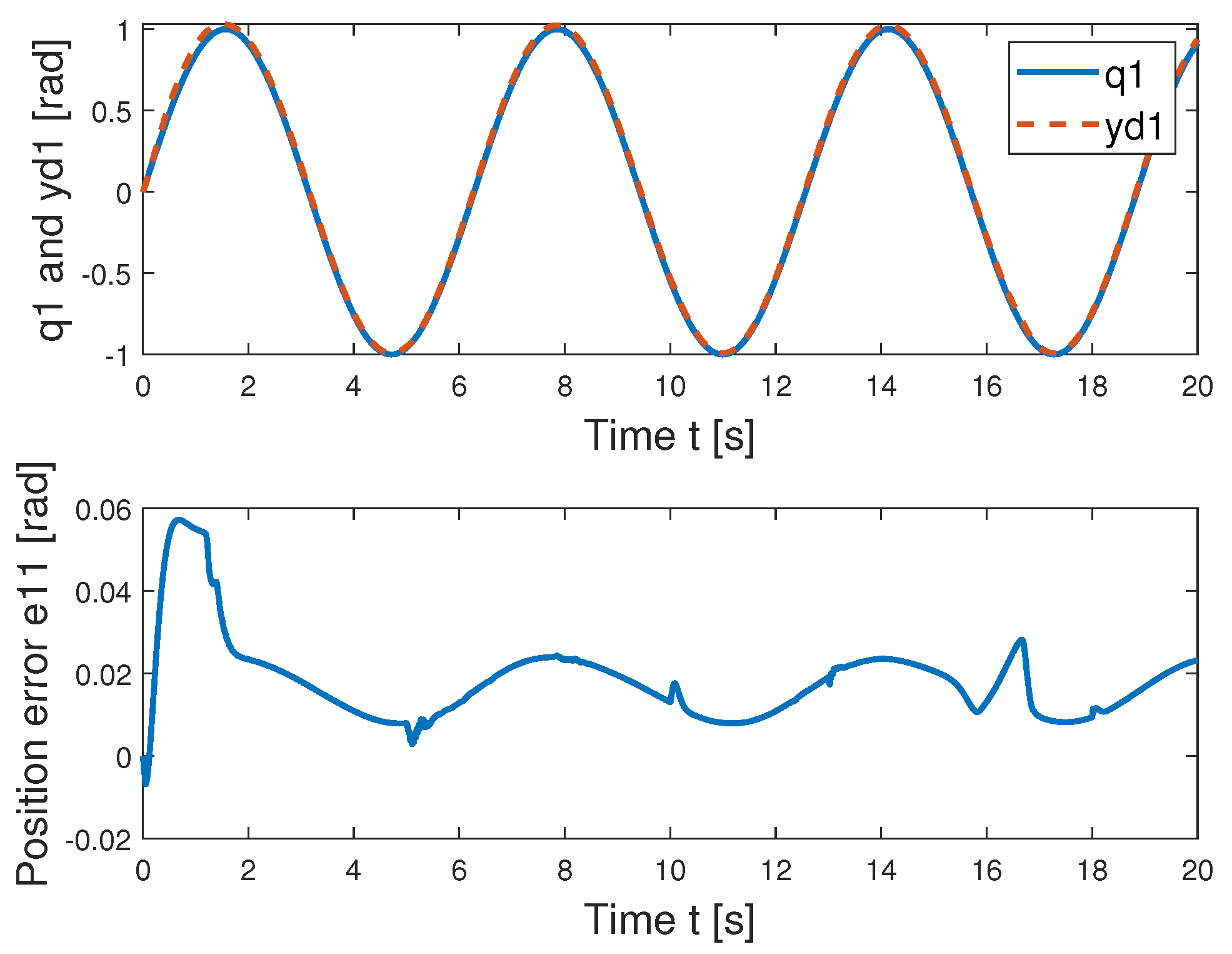
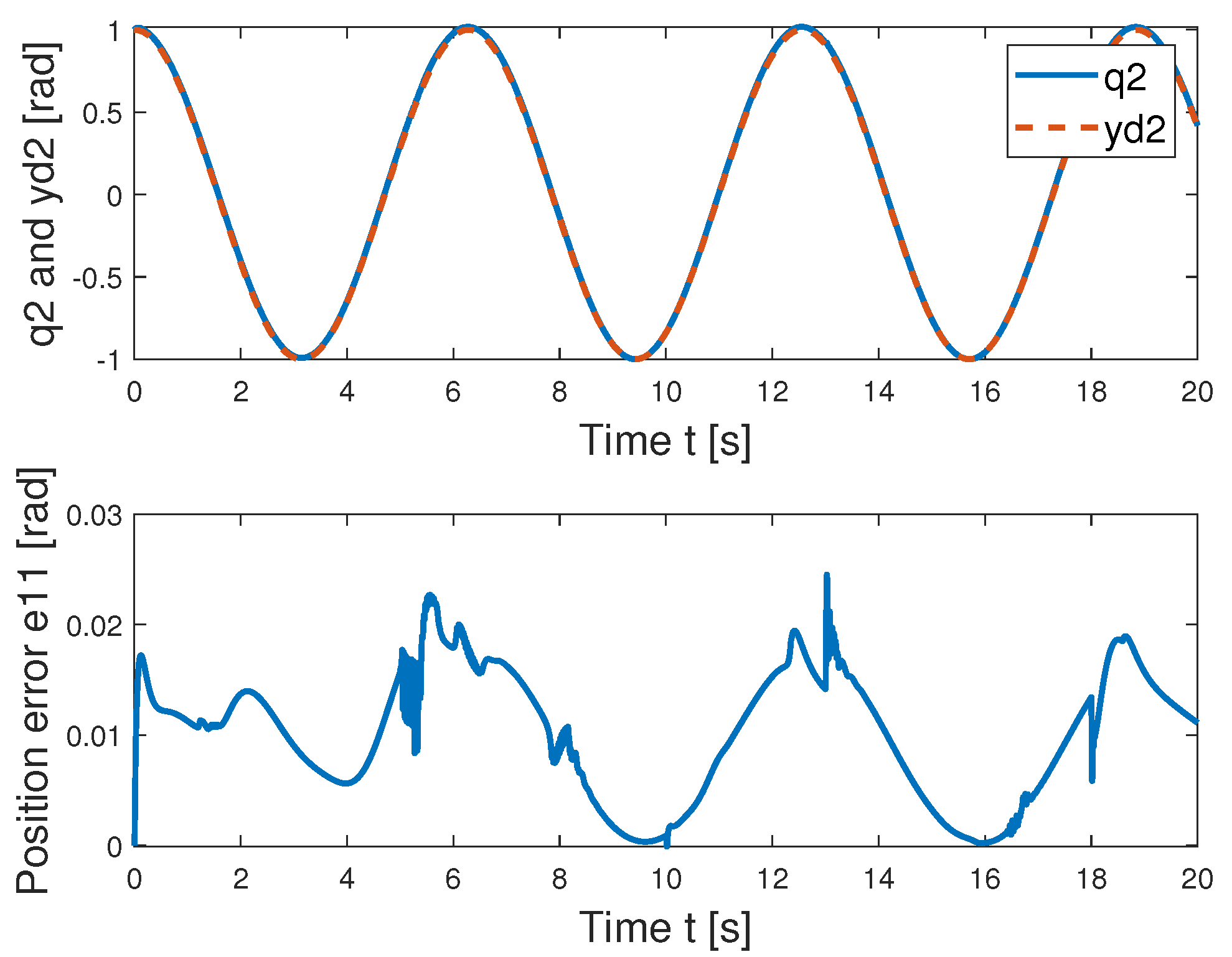
Step 1: First, the tracking error $e_1$ and the second error $e_2$ are defined as

$$e_1=x_1-y_d.$$

(14)

$$e_2=x_2-a_1.$$

(15)

where $a_1$ is a virtual control. The specific form is chosen as

$$a_1=-K_1{e}_1+\sum _{i=1}^n\frac{e_{1i}{\dot{b}}_{1i}}{b_{1i}}+{\dot{y}}_d,$$

(16)

where $K_1=\mathrm{diag}(K_{11},K_{12},\dots ,K_{1n})$ is a positive matrix. In order to achieve the control objectives, i.e., $|e_1|<\left|b_1\right|$, with $e_1={[e_{11},e_{12},\dots ,e_{1n}]}^T$ and $b_1={[b_{11},b_{12},\dots ,b_{1n}]}^T$, we construct the first Lyapunov function as

$$\begin{array}{cc}\hfill V_1& =\frac{1}{2}\sum _{i=1}^n\log \frac{b_{1i}^2}{b_{1i}^2-e_{1i}^2}.\hfill \end{array}$$

(17)

Then the derivative of (17) yields

$$\begin{array}{cc}\hfill {\dot{V}}_1& =\sum _{i=1}^n(-\frac{K_{1i}{e}_{1i}^2}{b_{1i}^2-e_{1i}^2}+\frac{e_{1i}{e}_{2i}}{b_{1i}^2-e_{1i}^2}).\hfill \end{array}$$

(18)

Step 2: The derivative of $e_2={[e_{21},e_{22},\dots ,e_{2n}]}^T$ is expressed as

$$\begin{array}{c}\hfill {\dot{e}}_2=M^{-1}[{\tau }_{SD}+\mathrm{\Lambda }+\varphi -C{\dot{x}}_1-G]-{\dot{a}}_1.\end{array}$$

(19)

We define the error $y_2$ between the output signal $a_{2O}$ and the input signal $a_{2I}$ of the first-order filter as

$$y_2=a_{2O}-a_{2I},$$

(20)

and a new error signal $e_3={[e_{31},e_{32},\dots ,e_{3n}]}^T$ is given as

$$\begin{array}{c}\hfill e_3={\tau }_{SD}-a_{2O}.\end{array}$$

(21)

Then ${\dot{e}}_2$ is rewritten as

$${\dot{e}}_2=M^{-1}[e_3+y_2+a_{2I}+\mathrm{\Lambda }+\varphi -C{x}_2-G]-\dot{a_1}.$$

(22)

Therefore, we design the virtual control law $a_{2I}$ as

$$\begin{array}{cc}\hfill a_{2I}=& -K_2{e}_2-{[\frac{e_{11}}{b_{11}^2-e_{11}^2},\frac{e_{12}}{b_{12}^2-e_{12}^2},\dots ,\frac{e_{1n}}{b_{1n}^2-e_{1n}^2}]}^T\hfill \\ \hfill & +C{a}_1+G+M{\dot{a}}_1-\overline{\mathrm{\Lambda }}\mathrm{sgn}\left(e_2\right)-\varphi ,\hfill \end{array}$$

(23)

where $K_2$ is the positive matrix with $K_2=\mathrm{diag}(K_{21},K_{22},\dots ,K_{2n})$.

In the above equation, we should know the upper bound $\overline{\mathrm{\Lambda }}$ in order to eliminate the effect of disturbance that is difficult to obtain in practice. To solve this problem, we utilize the adaptive scheme to approximate $\mathrm{\Lambda }$, and we define $\hat{\mathrm{\Lambda }}$ to be an estimated value, thus we have the approximate error

$$\tilde{\mathrm{\Lambda }}=\mathrm{\Lambda }-\hat{\mathrm{\Lambda }}.$$

(24)

Taking its derivative, we obtain

$$\dot{\tilde{\mathrm{\Lambda }}}=\dot{\mathrm{\Lambda }}-\dot{\hat{\mathrm{\Lambda }}}.$$

(25)

Then we design the adaptive law as

$$\dot{\hat{\mathrm{\Lambda }}}={\mathrm{\Gamma }}_{di}(e_{2i}+{\delta }_{di}\hat{\mathrm{\Lambda }}),$$

(26)

where ${\mathrm{\Gamma }}_{di}$ and ${\delta }_{di}$ are positive constants. The NNs are utilized to approximate the unknown parameter part of the system, and the control law is modified as

$$\begin{array}{cc}\hfill a_{2I}=& -K_2{e}_2-{[\frac{e_{11}}{b_{11}^2-e_{11}^2},\frac{e_{12}}{b_{12}^2-e_{12}^2},\dots ]}^T\hfill \\ \hfill & -\hat{\mathrm{\Lambda }}+{\widehat{W_{\tau }}}^T{S}_{\tau }\left(Z\right)+{\hat{W}}^{T}S\left(Z\right),\hfill \end{array}$$

(27)

and we define the approximate error $\widetilde{(•)}={(•)}^{*}-\widehat{(•)}$ so that

$$\begin{array}{cc}\hfill W^{*T}S\left(Z\right)& ={\hat{W}}^{T}S\left(Z\right)-\epsilon \hfill \\ \hfill & =C{a}_1+G+M{\dot{a}}_1-\epsilon ,\hfill \end{array}$$

(28)

$$\begin{array}{cc}\hfill W_{\tau }^{*T}S\left(Z_{\tau }\right)& ={\widehat{W_{\tau }}}^{T}S\left(Z_{\tau }\right)-{\epsilon }_{\tau }\hfill \\ \hfill & =\varphi -{\epsilon }_{\tau },\hfill \end{array}$$

(29)

where $Z={[x_1^T,x_2^T,a_1^T,{\dot{a}}_1^T]}^T$, $Z_{\tau }={[x_1^T,x_2^T,{e_1}^T,{\tau }_{SD}]}^T$. ${\hat{W}}^{T}S\left(Z\right),{\widehat{W_{\tau }}}^{T}S\left(Z_{\tau }\right)$ are the outputs of the network, and the updating law is designed as

$$\dot{\widehat{W_i}}=-{\mathrm{\Gamma }}_i[S_i\left(Z\right)e_{2,i}+{\sigma }_i{\hat{W}}_i],$$

(30)

$$\dot{\widehat{W_{\tau i}}}=-{\mathrm{\Gamma }}_{\tau i}[S_i\left(Z_{\tau }\right)e_{2,i}+{\sigma }_{\tau i}{\widehat{W_{\tau }}}_i],$$

(31)

where ${\mathrm{\Gamma }}_i={\mathrm{\Gamma }}_i^T>0$, ${\mathrm{\Gamma }}_{\tau i}={\mathrm{\Gamma }}_{\tau i}^T>0$, and ${\sigma }_i,{\sigma }_{\tau i}>0$.

Consider the second Lyapunov function candidate as

$$V_2=V_1+\frac{1}{2}{e}_2^{T}M\left(x_1\right)e_2+\frac{1}{2}{\tilde{\mathrm{\Lambda }}}^T{\mathrm{\Gamma }}^d\tilde{\mathrm{\Lambda }}+\frac{1}{2}\sum _{i=1}^n{\tilde{W}}_i^T{\mathrm{\Gamma }}_i^{-1}\widetilde{W_i}+\frac{1}{2}\sum _{i=1}^n{\tilde{W}}_{\tau i}^T{\mathrm{\Gamma }}_{\tau i}^{-1}\widetilde{W_{\tau i}}.$$

(32)

Taking the derivative of (32) yields

$$\begin{array}{cc}\hfill \dot{V_2}& \le -\sum _{i=1}^n\frac{K_{1i}{e}_{1i}^2}{b_{1i}^2-z_{1i}^2}-e_2^T(K_2-I_{n\times n})e_2\hfill \\ \hfill & +e_2^T{y}_2+e_2^T{e}_3-\sum _{i=1}^n\frac{{\sigma }_i}{2}{∥{\tilde{W}}_i∥}^2-\sum _{i=1}^n\frac{{\sigma }_{\tau i}}{2}{∥{\widetilde{W_{\tau }}}_i∥}^2\hfill \\ \hfill & +\sum _{i=1}^n\frac{{\sigma }_i}{2}{∥W_i^{*}∥}^2+\sum _{i=1}^n\frac{{\sigma }_{\tau i}}{2}{∥{W_{\tau }}_i^{*}∥}^2+\frac{1}{2}{∥\overline{\epsilon }∥}^2+\frac{1}{2}{∥\overline{{\epsilon }_{\tau }}∥}^2\hfill \\ \hfill & -\frac{1}{2}\sum _{i=1}^n\left({\delta }_{di}-{\mathrm{\Gamma }}_{di}^{-1}\right){\tilde{\mathrm{\Lambda }}}_i^2+\frac{1}{2}\sum _{i=1}^n{\mathrm{\Gamma }}_{di}^{-1}{b}_{1i}^2+\frac{1}{2}\sum _{i=1}^n{\delta }_{di}{\overline{\mathrm{\Lambda }}}_i^2.\hfill \end{array}$$

(33)

Then we obtain

$$\begin{array}{cc}\hfill \dot{V_2}& \le -\sum _{i=1}^n\frac{K_{1i}{e}_{1i}^2}{b_{1i}^2-z_{1i}^2}-e_2^T(K_2-I_{n\times n})e_2\hfill \\ \hfill & +e_2^T{y}_2+e_2^T{e}_3-\sum _{i=1}^n\frac{{\sigma }_i}{2}{∥{\tilde{W}}_i∥}^2-\sum _{i=1}^n\frac{{\sigma }_{\tau i}}{2}{∥{\widetilde{W_{\tau }}}_i∥}^2\hfill \\ \hfill & -\frac{1}{2}\sum _{i=1}^n\left({\delta }_{di}-{\mathrm{\Gamma }}_{di}^{-1}\right){\tilde{\mathrm{\Lambda }}}_i^2+C_2,\hfill \end{array}$$

(34)

where

$$\begin{array}{c}\hfill C_2=\sum _{i=1}^n\frac{{\sigma }_i}{2}{∥W_i^{*}∥}^2+\sum _{i=1}^n\frac{{\sigma }_{\tau i}}{2}{∥{W_{\tau }}_i^{*}∥}^2+\frac{1}{2}{∥\overline{\epsilon }∥}^2+\frac{1}{2}{∥\overline{{\epsilon }_{\tau }}∥}^2+\frac{1}{2}\sum _{i=1}^n{\mathrm{\Gamma }}_{di}^{-1}{b}_{1i}^2+\frac{1}{2}\sum _{i=1}^n{\delta }_{di}{\overline{\mathrm{\Lambda }}}_i^2\end{array}$$

(35)

Step 3: Consider the final Lyapunov function $V_3$ as

$$V_3=V_2+\frac{1}{2}{e}_3^T{e}_3+\frac{1}{2}{y}_2^T{y}_2.$$

(36)

In order to obtain the derivative of $a_{2I}$, we pass the virtual control signal $a_{2I}$ through the finite-time first order filter with positive constants ${\alpha }_2$ and ${\beta }_2$ as

$$\begin{array}{c}\hfill {\dot{a}}_{2O}=-{\alpha }_2(a_{2O}-a_{2I})-{\beta }_2{(a_{2O}-a_{2I})}^{q/p},a_{2O}\left(0\right)=a_{2I}\left(0\right).\end{array}$$

(37)

We utilize the Nussbaum function to convert $\omega$

$$\begin{array}{cc}\hfill N\left(\chi \right)& ={\chi }^{2}cos\left(\chi \right),\hfill \\ \hfill \dot{\chi }& ={\gamma }_{\chi }{e}_3\overline{\omega },\hfill \\ \hfill \omega & =N\left(\chi \right)\overline{\omega },\hfill \end{array}$$

(38)

where ${\gamma }_{\chi }>0$ is positive constant, and $\overline{\omega }$ is an auxiliary control signal vector.

$\overline{\omega }$ is constructed as

$$\overline{\omega }=-K_3{e}_3-e_2+p_{SD}cv+{\dot{a}}_{2O},$$

(39)

where $K_3=\mathrm{diag}(K_{31},K_{32},\dots ,K_{3n})$ is the positive matrix and $p_{SD}=\mathrm{diag}(\frac{\partial {\tau }_{SD1}}{\partial v_1},\frac{\partial {\tau }_{SD2}}{\partial v_2},\dots ,\frac{\partial {\tau }_{SDn}}{\partial v_n})$.

Then we take the derivative of $V_3$

$$\begin{array}{cc}\hfill \dot{V_3}& \le -\sum _{i=1}^n\frac{K_{1i}{e}_{1i}^2}{b_{1i}^2-z_{1i}^2}-e_2^T(K_2-\frac{3}{2}{I}_{n\times n})e_2-e_3^T{K}_3{e}_3\hfill \\ \hfill & -\sum _{i=1}^n\frac{{\sigma }_i}{2}{∥{\tilde{W}}_i∥}^2-\sum _{i=1}^n\frac{{\sigma }_{\tau i}}{2}{∥{\widetilde{W_{\tau }}}_i∥}^2-\frac{1}{2}\sum _{i=1}^n\left({\delta }_{di}-{\mathrm{\Gamma }}_{di}^{-1}\right){\tilde{\mathrm{\Lambda }}}_i^2\hfill \\ \hfill & +\sum _{i=1}^n\frac{{\dot{\chi }}_i}{{\gamma }_{\chi i}}(p_{g_i^v}{N}_i\left({\chi }_i\right)-1)+(1-{\alpha }_2)y_2^T{y}_2+C_3,\hfill \end{array}$$

(40)

where $C_3=C_2+\frac{1}{2}{\eta }_2^T{\eta }_2$, and ${\eta }_2$ is the nonnegative continuous function such that

$$\begin{array}{cc}\hfill |{\dot{a}}_{2I}|& \le {\eta }_2(z_1,e_2,\widehat{W_i},y_d,\dot{y_d},\ddot{y_d}).\hfill \end{array}$$

(41)

Finally, we obtain

$$\begin{array}{cc}\hfill \dot{V_3}& \le -\rho V_3+\sum _{i=1}^n\frac{{\dot{\chi }}_i}{{\gamma }_{\chi i}}(p_{g_i^v}{N}_i\left({\chi }_i\right)-1)+C_3,\hfill \end{array}$$

(42)

where

$$\begin{array}{cc}\hfill \rho =& min[min(2K_{1i}),min(\frac{{\lambda }_{min}(2K_2-3I_{n\times n})}{{\lambda }_{max}\left(M\right)}),min\left(2K_{3i}\right),\hfill \\ \hfill & min(\frac{{\sigma }_i}{{\lambda }_{max}\left({\mathrm{\Gamma }}_i^{-1}\right)}),min(\frac{{\sigma }_{\tau i}}{{\lambda }_{max}\left({\mathrm{\Gamma }}_{\tau i}^{-1}\right)}),min(\frac{{\delta }_{di}-{\mathrm{\Gamma }}_{di}^{-1}}{{\lambda }_{max}\left({\mathrm{\Gamma }}_d^{-1}\right)}),2(1-{\alpha }_2)].\hfill \end{array}$$

(43)

Integrating (42) gives

$$\begin{array}{c}\hfill V_3\left(t\right)-V_3\left(0\right)\le -\rho {\int }_0^t{V}_3\left(\tau \right)d\tau +O,\end{array}$$

(44)

where $O=\int {\sum }_{i=1}^n\frac{{\dot{\chi }}_i}{{\gamma }_{\chi i}}(p_{g_i^v}{N}_i\left({\chi }_i\right)-1)dt$. From [45], $\chi$ is bounded, so O is bounded, and in turn we determine that there exists an upper bound Q for $V_3$ such that

$$\begin{array}{cc}\hfill \frac{1}{2}\sum _{i=1}^{n}log\frac{b_{1i}^2}{b_{1i}^2-e_{1i}^2}& \le V_3\le Q,\hfill \\ \hfill \frac{1}{2}{e}_2^{T}M{e}_2& \le V_3\le Q.\hfill \end{array}$$

(45)

Then the error signals $e_1$ and $e_2$ are kept within the compact set ${\mathrm{\Omega }}_{e_1}$ and ${\mathrm{\Omega }}_{e_2}$

$$\begin{array}{cc}\hfill {\mathrm{\Omega }}_{e_1}:& =\left\{e_{1i}\in {\mathbb{R}}^n\mid ∥e_{1i}∥\le \sqrt{b_{1i}^2\left(1-e^{-2Q}\right)}\right\},\hfill \\ \hfill {\mathrm{\Omega }}_{e_2}:& =\left\{e_2\in {\mathbb{R}}^n\mid ∥e_2∥\le \sqrt{\frac{2Q}{{\lambda }_{min}\left(M\right)}}\right\}.\hfill \end{array}$$

(46)

Similarly, we can determine that the errors $e_3,\tilde{\mathrm{\Lambda }},\tilde{W},$ and $\widetilde{W_{\tau }}$ are bounded. Therefore, we can conclude that the tracking errors and the approximate errors of the system converge to zero under the conditions of the proposed control law and suitable parameters.

4. Simulations

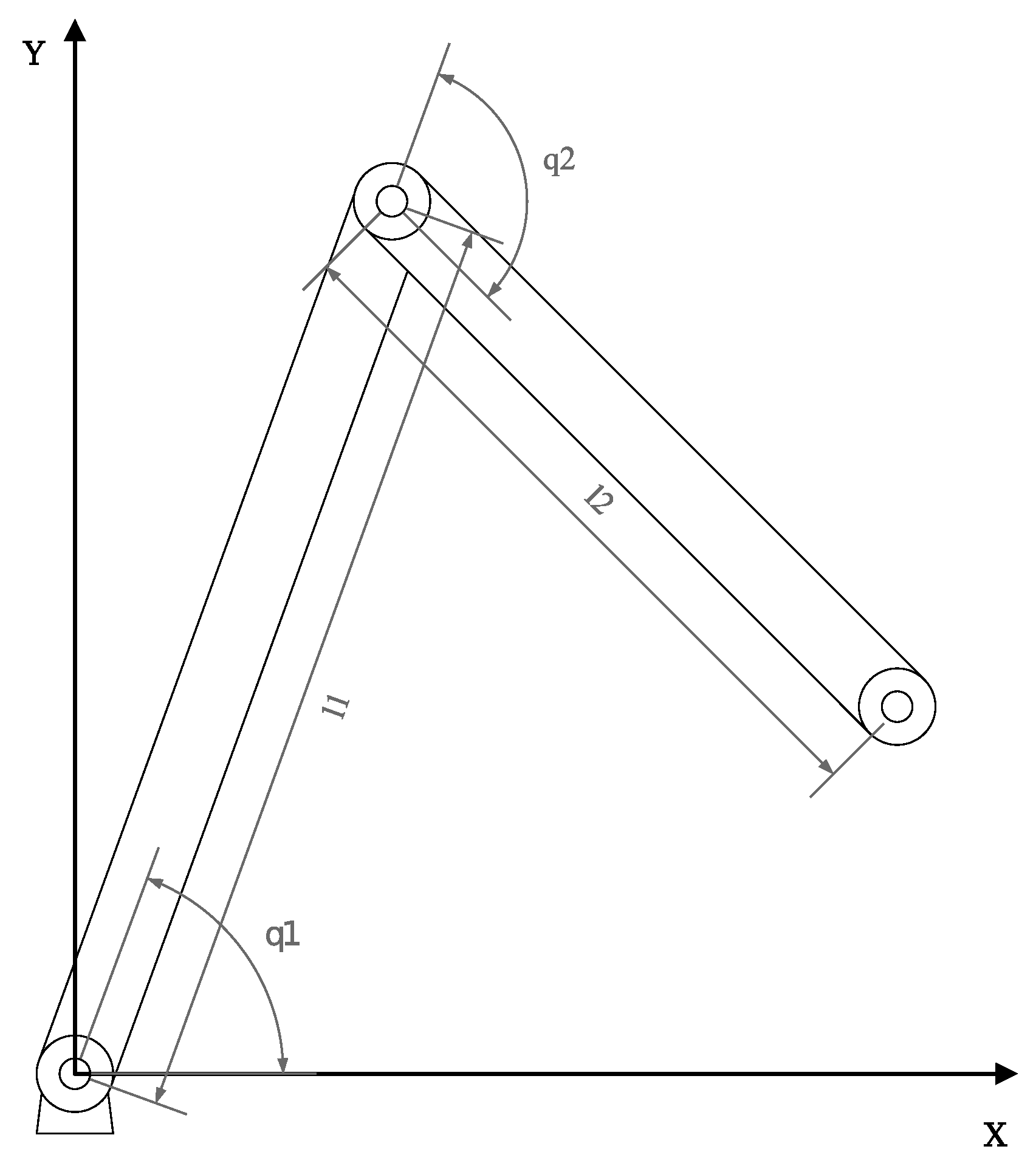
4.1. Robotic System Establishment

In the simulation part, using the robotic arm model in [46], the structure is shown in Figure 2. The descriptions of inertia matrix $M\left(q\right)$, Centripetal and Coriolis torques matrix $C(q,\dot{q})$, and gravitational force vector $G\left(q\right)$ are provided as

$$\begin{array}{c}\hfill M\left(q\right)=\left[\begin{array}{cc}{M}_{11}& M_{12}\\ M_{21}& M_{22}\end{array}\right],\end{array}$$

(47)

$$\begin{array}{c}\hfill C(q,\dot{q})=\left[\begin{array}{cc}{C}_{11}& C_{12}\\ C_{21}& C_{22}\end{array}\right],\end{array}$$

(48)

$$\begin{array}{c}\hfill G\left(q\right)=\left[\begin{array}{c}{G}_{11}\\ G_{21}\end{array}\right],\end{array}$$

(49)

and

$$\begin{array}{cc}\hfill & M_{11}=m_1{l}_{c1}^2+m_2\left(l_1^2+l_{c2}^2+2l_1{l}_{c2}cos{q}_2\right)+I_1+I_2,\hfill \\ \hfill & M_{12}=m_2\left(l_{c2}^2+l_1{l}_{c2}cos{q}_2\right)+I_2,\hfill \\ \hfill & M_{21}=m_2\left(l_{c2}^2+l_1{l}_{c2}cos{q}_2\right)+I_2,\hfill \\ \hfill & M_{22}=m_2{l}_{c2}^2+I_2,\hfill \\ \hfill & C_{11}=-m_2{l}_1{l}_{c2}{\dot{q}}_{2}sin{q}_2,\hfill \\ \hfill & C_{12}=-m_2{l}_1{l}_{c2}\left({\dot{q}}_1+{\dot{q}}_2\right)sin{q}_2,\hfill \\ \hfill & C_{21}=m_2{l}_1{l}_{c2}{\dot{q}}_{1}sin{q}_2,\hfill \\ \hfill & C_{22}=0,\hfill \\ \hfill & G_{11}=\left(m_1{l}_{c2}+m_2{l}_1\right)gcos{q}_1+m_2{l}_{c2}gcos\left(q_1+q_2\right),\hfill \\ \hfill & G_{21}=m_2{l}_{c2}gcos\left(q_1+q_2\right).\hfill \end{array}$$

(50)

The structural parameters of the robot are shown in

Table 1. Parameters of the robot.

Parameter	Description	Value
$m_1$	Mass of link 1	2.00 kg
$m_2$	Mass of link 2	0.85 kg
$l_1$	Length of link 1	0.35 m
$l_2$	Length of link 2	0.31 m
$I_1$	Moment of inertia of link 1	$\frac{1}{4}{m}_1{l}_1^2$ kgm2
$I_2$	Moment of inertia of link 2	$\frac{1}{4}{m}_2{l}_2^2$ kgm2

, and the initial state is set as

$$q_1\left(0\right)=0,q_2\left(0\right)=1,{\dot{q}}_1\left(0\right)=1,{\dot{q}}_2\left(0\right)=0.$$

(51)

The desired tracking trajectory is given as $y_d={[sin\left(t\right),cos\left(t\right)]}^T$, where $t\in [0,t_s]$ and $t_s=20$ s. The other conditions and parameters are taken as $K_1=\mathrm{diag}(7,3)$, $K_2=\mathrm{diag}(10,5)$, $K_3=\mathrm{diag}(15,10)$, and $c=2$. The disturbance is given as $\mathrm{\Lambda }={[0.5sin\left(t\right)+1,0.5cos\left(t\right)+0.5]}^T$. Further, to describe the error signals during actuator operation, we consider the following form of $\varphi$

$$\varphi =\left\{\begin{array}{cc}-0.4{\tau }_{SD},\hfill & t\in [5,10]\hfill \\ -0.4{\tau }_{SD}+{[2cos\left(t\right),2]}^T.\hfill & t\in [13,18]\hfill \end{array}\right.$$

(52)

4.2. Model-Based Control

For the model-based (MB) control, we use the MB control designed in (23), and then the other parameters are set as $p=15$, $q=11$, ${\alpha }_2=40$, and ${\beta }_2=40$. The saturation value of the actuator $u_M$ is set as $\mathrm{diag}(13,10)$. The dead zone characteristic parameters are set as $k={[1,1]}^T$, $r={[2,3]}^T$, ${\zeta }_l={[2,1]}^T$, and ${\zeta }_r={[10,3]}^T$, and the time-varying output constraints are $b_1={[0.8\exp (-5t)+0.2,0.8\exp (-5t)+0.2]}^T$. The initial conditions are taken as $a_{2O}\left(0\right)=0,\hat{\mathrm{\Lambda }}\left(0\right)={[0,0]}^T$.

The simulation results are illustrated in Figure 3, Figure 4, Figure 5 and Figure 6. According to Figure 3 and Figure 4, it can be seen that the system has good position tracking performance. The position output errors do not violate the time-varying output constraints, and the errors can be kept to a minimum during periods of actuator failure. Figure 5 and Figure 6 illustrate the relationship between the system inputs and actuator inputs. The system input signals always stay within the saturation interval, and the control signals fluctuate widely at moments of sudden change.

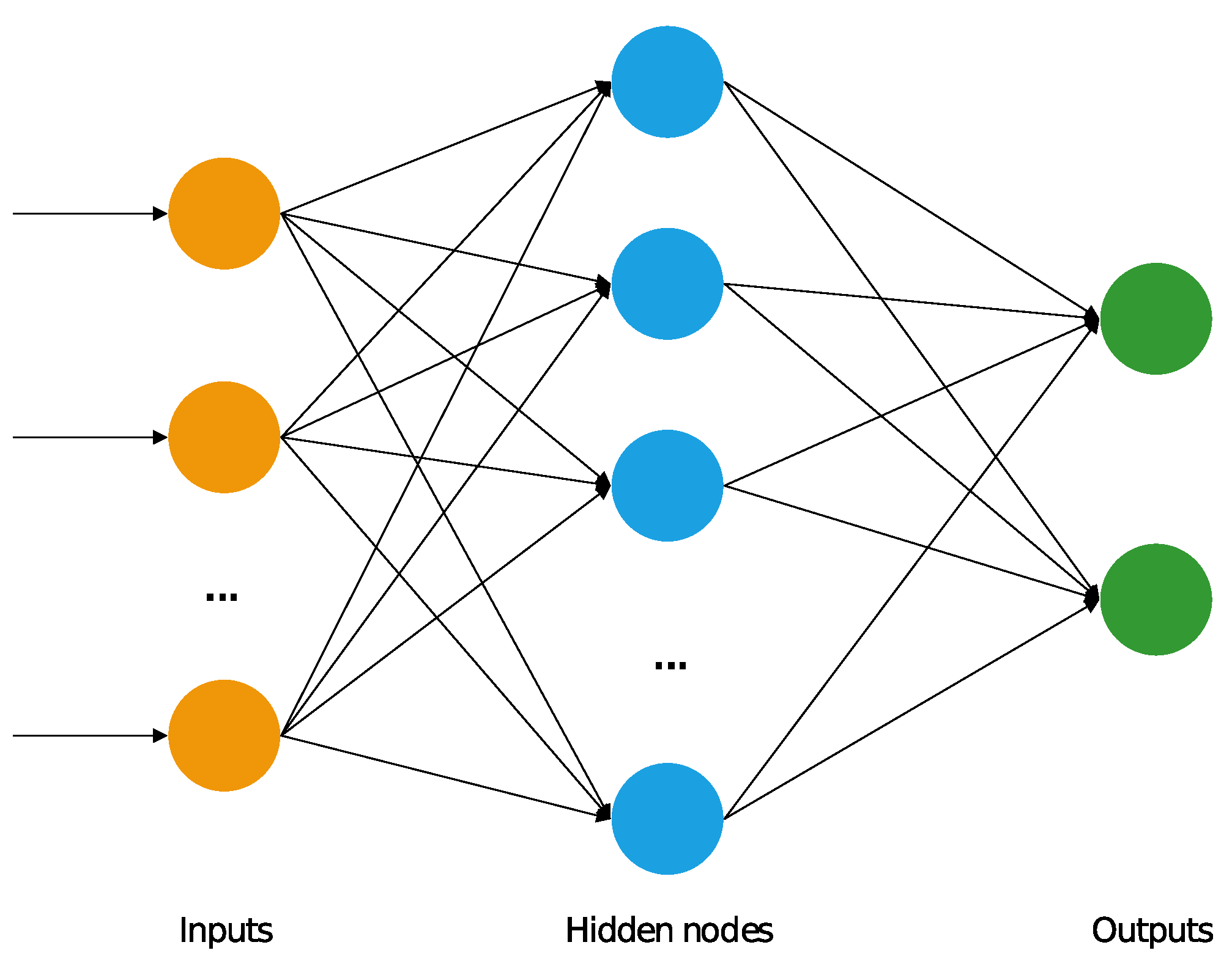
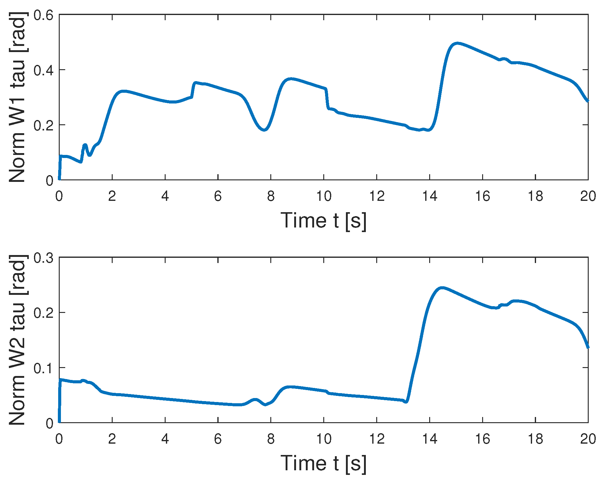
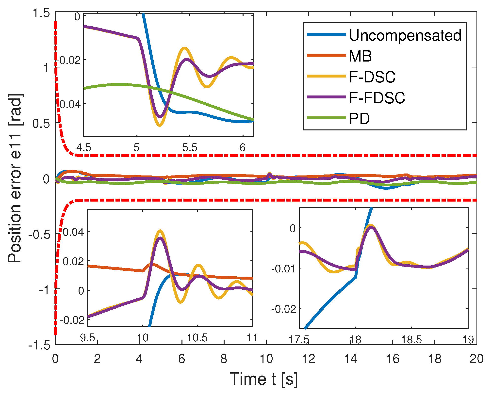
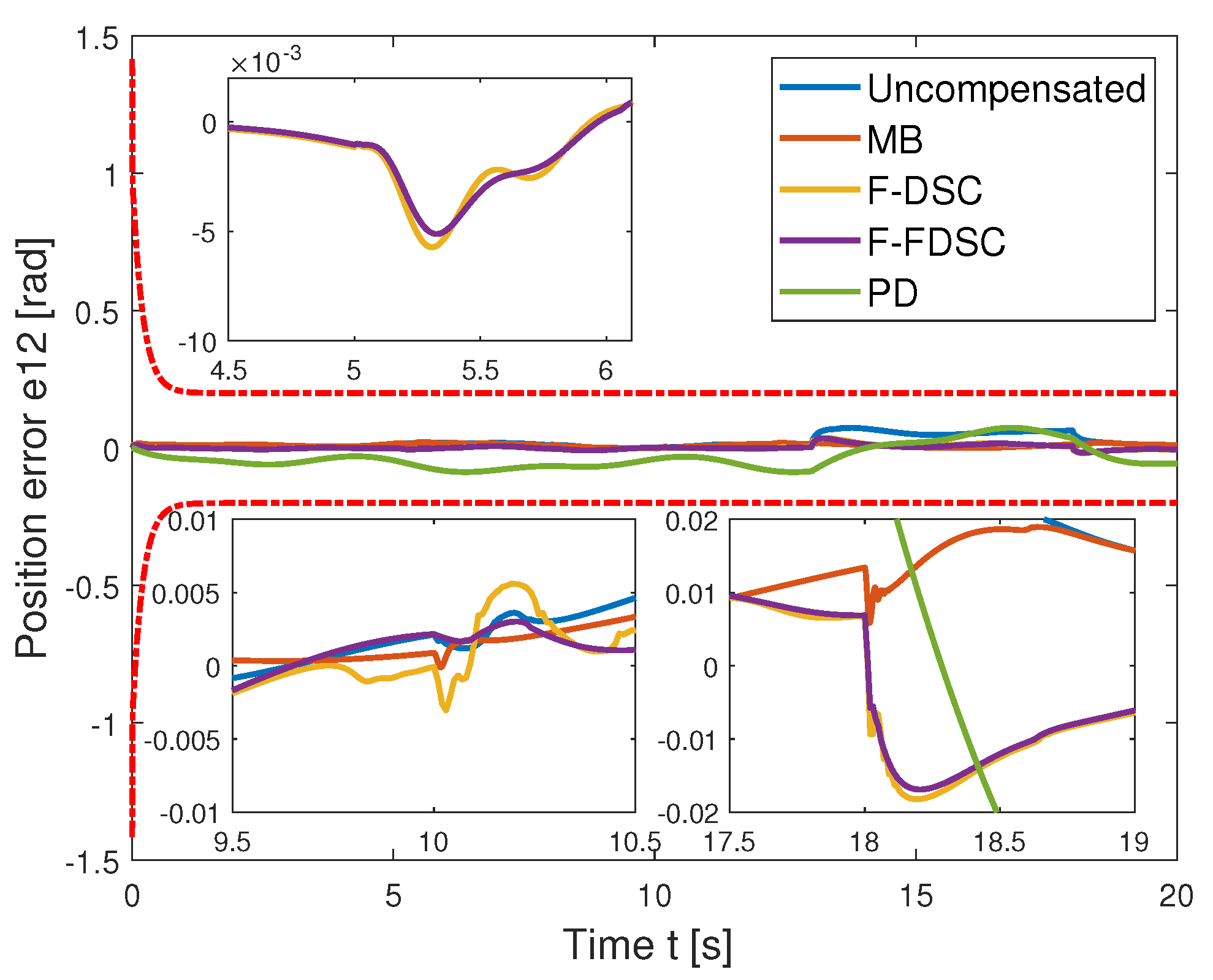
4.3. Adaptive Neural Network Control

For NNs control, we use the control law (27) with the update law (30) and (31). The constraint and gain parameters are the same as those of the MB control, and the control process is shown in Figure 7. The initial conditions are taken as $\hat{W}\left(0\right)=0$, $\widehat{W_{\tau }}\left(0\right)=0$, $a_{2O}\left(0\right)=0,\hat{\mathrm{\Lambda }}\left(0\right)={[0,0]}^T$. $S\left(Z\right)$ and $S\left(Z_{\tau }\right)$ both have 256 nodes; the node centers of NNs ${\mu }_{ki},i=(1,2,\dots ,8)$ are selected in the area of $[-1,1]\times [-1,1]\times [-1,1]\times [-1,1]\times [-1,1]\times [-1,1]\times [-1,1]\times [-1,1]$, ${\eta }_k=2$. The other parameters are given as

$$\begin{array}{c}\hfill \mathrm{\Gamma }=10I_{256\times 256},\sigma =[0.01;0.01],\\ \hfill {\mathrm{\Gamma }}_{\tau }=50I_{256\times 256},{\sigma }_{\tau }=[0.02;0.02].\end{array}$$

(53)

The position tracking performance is shown in Figure 8 and Figure 9, while the corresponding actuator input v and the system input ${\tau }_{SD}$ are displayed in Figure 10 and Figure 11. Compared with the control strategy of MB, the neural network-based control method reduces the fluctuation of the control signal to a certain extent. Figure 12 and Figure 13 depict the weights of the NNs approximation W and $W_{\tau }$.

4.4. PD Control

This case considers a PD controller with a specific control law as $\tau =-K_p{e}_1-K_d{\dot{e}}_1$, where $K_p=\mathrm{diag}(150,20),K_d=\mathrm{diag}(50,20)$. We compare the tracking errors for several different cases with the same control constraints (uncompensated for faults, MB control (23), fault-tolerant DSC (F-DSC) (${\beta }_2=0$), fault-tolerant finite-time DSC (F-FDSC) (27), and PD control) in Figure 14 and Figure 15. First, when compared to the uncompensated, the employment of the NNs approach to compensate for the fault signal improves system performance during the fault time. Second, when the actuator’s state changes, F-FDSC can make the tracking error enter the steady state more smoothly and reduce the error fluctuation compared to F-DSC.

Finally, we sorted out in

Table 2. Output error values.

Parameter	${\mathit{e}}_{11}$ [rad]	${\mathit{e}}_{12}$ [rad]
Uncompensated	0.0936	0.0738
MB	0.0282	0.0245
F-DSC	0.0498	0.0366
F-FDSC	0.0460	0.0360
PD	0.0635	0.0872

the maximum tracking error values E for the above methods during the period of actuator failure, where $E=max\left|x_1-y_d\right|$. By comparison, it can be seen that NNs fault-tolerant control is better than the traditional PD control.

5. Conclusions

In this study, a neural-network-based fault-tolerant controller was proposed for a robotic manipulator system with multiple constraints and actuator failures. A finite-time DSC filter was employed to optimize the design process and ensure that the output of the system converged quickly, even if actuator failure occurred. The neural network approach was applied to approximate actuator faults and uncertain robotic parameters, and a disturbance observer was used to eliminate the effects of external disturbances. Finally, the effectiveness of the proposed controller was demonstrated by the simulation results, that is, the system remained stable and the constraints were never violated, it had better performance during the actuator failure period, and the error signal could enter the steady state faster. The digital simulation initially verifies the feasibility of the designed controller, which we will also verify in real systems in the future.

References

1. Zhang, T.; Ge, S. Adaptive dynamic surface control of nonlinear systems with unknown dead zone in pure feedback form. Automatica 2008, 44, 1895–1903. [Google Scholar] [CrossRef]
2. Wang, L.; Shi, Q.; Liu, J.; Zhang, D. Backstepping control of flexible joint manipulator based on hyperbolic tangent function with control input and rate constraints. Asian J. Control 2020, 22, 1268–1279. [Google Scholar] [CrossRef]
3. Wei, H.; Amoateng, D.O.; Yang, C.; Gong, D. Adaptive neural network control of a robotic manipulator with unknown backlash-like hysteresis. IET Control Theory Appl. 2017, 11, 567–575. [Google Scholar]
4. Yang, C.; Huang, D.; He, W.; Cheng, L. Neural Control of Robot Manipulators with Trajectory Tracking Constraints and Input Saturation. IEEE Trans. Neural Netw. Learn. Syst. 2021, 32, 4231–4242. [Google Scholar] [CrossRef] [PubMed]
5. Zhao, Z.; He, X.; Ren, Z.; Wen, G. Boundary Adaptive Robust Control of a Flexible Riser System with Input Nonlinearities. IEEE Trans. Syst. Man Cybern. Syst. 2019, 49, 1971–1980. [Google Scholar] [CrossRef]
6. Zhao, Z.; Zhang, J.; Liu, Z.; Mu, C.; Hong, K.-S. Adaptive Neural Network Control of an Uncertain 2-DOF Helicopter with Unknown Backlash-like Hysteresis and Output Constraints. IEEE Trans. Neural Netw. Learn. Syst. 2022. [Google Scholar] [CrossRef] [PubMed]
7. Tao, G.; Kokotovic, P. Adaptive control of plants with unknown dead-zones. IEEE Trans. Autom. Control 1994, 39, 59–68. [Google Scholar]
8. Zhou, J.; Wen, C.; Zhang, Y. Adaptive Output Control of Nonlinear Systems with Uncertain Dead-Zone Nonlinearity. IEEE Trans. Autom. Control 2006, 51, 504–511. [Google Scholar] [CrossRef]
9. Shi, Z. Global Asymptotic Tracking for Gear Transmission Servo Systems with Differentiable Backlash Nonlinearity. In Proceedings of the 2014 Seventh International Symposium on Computational Intelligence and Design, Hangzhou, China, 13–14 December 2014; Volume 2, pp. 253–257. [Google Scholar] [CrossRef]
10. Jin, C.; Cai, M.; Xu, Z. Dual-Motor Synchronization Control Design Based on Adaptive Neural Networks Considering Full-State Constraints and Partial Asymmetric Dead-Zone. Sensors 2021, 21, 4261. [Google Scholar] [CrossRef]
11. Shi, X.; Lim, C.C.; Shi, P.; Xu, S. Adaptive Neural Dynamic Surface Control for Nonstrict-Feedback Systems with Output Dead Zone. IEEE Trans. Neural Netw. Learn. Syst. 2018, 29, 5200–5213. [Google Scholar] [CrossRef] [PubMed] [Green Version]
12. Lu, K.; Liu, Z.; Lai, G.; Zhang, Y.; Chen, C.L.P. Adaptive Fuzzy Tracking Control of Uncertain Nonlinear Systems Subject to Actuator Dead Zone with Piecewise Time-Varying Parameters. IEEE Trans. Fuzzy Syst. 2019, 27, 1493–1505. [Google Scholar] [CrossRef]
13. Liu, Z.; Wang, F.; Zhang, Y.; Chen, X.; Chen, C.L.P. Adaptive Tracking Control for A Class of Nonlinear Systems with a Fuzzy Dead-Zone Input. IEEE Trans. Fuzzy Syst. 2015, 23, 193–204. [Google Scholar] [CrossRef]
14. Hua, C.; Wang, Q.; Guan, X. Adaptive Tracking Controller Design of Nonlinear Systems with Time Delays and Unknown Dead-Zone Input. IEEE Trans. Autom. Control 2008, 53, 1753–1759. [Google Scholar] [CrossRef]
15. Yao, D.; Dou, C.; Zhao, N.; Zhang, T. Finite-time consensus control for a class of multi-agent systems with dead-zone input. J. Frankl. Inst. 2021, 358, 3512–3529. [Google Scholar] [CrossRef]
16. Zhao, Z.; Ren, Y.; Mu, C.; Zou, T.; Hong, K.S. Adaptive Neural-Network-Based Fault-Tolerant Control for a Flexible String with Composite Disturbance Observer and Input Constraints. IEEE Trans. Cybern. 2021, 1–11. [Google Scholar] [CrossRef]
17. Zhao, Z.; Liu, Z.; He, W.; Hong, K.S.; Li, H.X. Boundary adaptive fault-tolerant control for a flexible Timoshenko arm with backlash-like hysteresis. Automatica 2021, 130, 109690. [Google Scholar] [CrossRef]
18. Chen, S.; Zhao, Z.; Zhu, D.; Zhang, C.; Li, H.X. Adaptive Robust Control for a Spatial Flexible Timoshenko Manipulator Subject to Input Dead-Zone. IEEE Trans. Syst. Man Cybern. Syst. 2022, 52, 1395–1404. [Google Scholar] [CrossRef]
19. Ma, H.J.; Yang, G.H. Adaptive output control of uncertain nonlinear systems with non-symmetric dead-zone input. Automatica 2010, 46, 413–420. [Google Scholar] [CrossRef]
20. Chen, Y.; Liu, Z.; Chen, C.; Zhang, Y. Adaptive fuzzy control of switched nonlinear systems with uncertain dead-zone: A mode-dependent fuzzy dead-zone model. Neurocomputing 2021, 432, 133–144. [Google Scholar] [CrossRef]
21. He, W.; Ouyang, Y.; Hong, J. Vibration Control of a Flexible Robotic Manipulator in the Presence of Input Deadzone. IEEE Trans. Ind. Inform. 2017, 13, 48–59. [Google Scholar] [CrossRef]
22. Yang, C.; Peng, G.; Cheng, L.; Na, J.; Li, Z. Force Sensorless Admittance Control for Teleoperation of Uncertain Robot Manipulator Using Neural Networks. IEEE Trans. Syst. Man Cybern. Syst. 2021, 51, 3282–3292. [Google Scholar] [CrossRef]
23. He, W.; Kong, L.; Dong, Y.; Yu, Y.; Yang, C.; Sun, C. Fuzzy Tracking Control for a Class of Uncertain MIMO Nonlinear Systems with State Constraints. IEEE Trans. Syst. Man Cybern. Syst. 2019, 49, 543–554. [Google Scholar] [CrossRef]
24. Kong, L.; Wei, H.; Yang, C.; Li, G.; Zhang, Z. Adaptive Fuzzy Control for a Marine Vessel with Time-varying Constraints. IET Control Theory Appl. 2018, 12, 1448–1455. [Google Scholar] [CrossRef]
25. Yang, C.; Chen, C.; Wang, N.; Ju, Z.; Fu, J.; Wang, M. Biologically Inspired Motion Modeling and Neural Control for Robot Learning From Demonstrations. IEEE Trans. Cogn. Dev. Syst. 2019, 11, 281–291. [Google Scholar] [CrossRef] [Green Version]
26. He, W.; Chen, Y.; Yin, Z. Adaptive Neural Network Control of an Uncertain Robot with Full-State Constraints. IEEE Trans. Cybern. 2016, 46, 620–629. [Google Scholar] [CrossRef]
27. He, W.; Huang, H.; Ge, S.S. Adaptive Neural Network Control of a Robotic Manipulator with Time-Varying Output Constraints. IEEE Trans. Cybern. 2017, 47, 3136–3147. [Google Scholar] [CrossRef]
28. He, W.; Yin, Z.; Sun, C. Adaptive Neural Network Control of a Marine Vessel with Constraints Using the Asymmetric Barrier Lyapunov Function. IEEE Trans. Cybern. 2017, 47, 1641–1651. [Google Scholar] [CrossRef]
29. Mao, Z.; Yan, X.G.; Jiang, B.; Chen, M. Adaptive Fault-Tolerant Sliding-Mode Control for High-Speed Trains with Actuator Faults and Uncertainties. IEEE Trans. Intell. Transp. Syst. 2020, 21, 2449–2460. [Google Scholar] [CrossRef] [Green Version]
30. Li, L.; Liu, J. Neural-network-based adaptive fault-tolerant vibration control of single-link flexible manipulator. Trans. Inst. Meas. Control 2020, 42, 430–438. [Google Scholar] [CrossRef]
31. Zhang, S.; Yang, P.; Kong, L.; Li, G.; He, W. A Single Parameter-Based Adaptive Approach to Robotic Manipulators with Finite Time Convergence and Actuator Fault. IEEE Access 2020, 8, 15123–15131. [Google Scholar] [CrossRef]
32. Wang, J.; Liu, Z.; Chen, C.L.P.; Zhang, Y. Fuzzy Adaptive Compensation Control of Uncertain Stochastic Nonlinear Systems with Actuator Failures and Input Hysteresis. IEEE Trans. Cybern. 2019, 49, 2–13. [Google Scholar] [CrossRef] [PubMed]
33. Zhang, S.; Yang, P.; Kong, L.; Chen, W.; Fu, Q.; Peng, K. Neural Networks-Based Fault Tolerant Control of a Robot via Fast Terminal Sliding Mode. IEEE Trans. Syst. Man Cybern. Syst. 2021, 51, 4091–4101. [Google Scholar] [CrossRef]
34. Liu, L.; Liu, Y.J.; Tong, S. Neural Networks-Based Adaptive Finite-Time Fault-Tolerant Control for a Class of Strict-Feedback Switched Nonlinear Systems. IEEE Trans. Cybern. 2019, 49, 2536–2545. [Google Scholar] [CrossRef] [PubMed]
35. Ren, Y.; Zhu, P.; Zhao, Z.; Yang, J.; Zou, T. Adaptive Fault-Tolerant Boundary Control for a Flexible String with Unknown Dead Zone and Actuator Fault. IEEE Trans. Cybern. 2021, 1–10. [Google Scholar] [CrossRef] [PubMed]
36. Hu, Q.; Shao, X.; Guo, L. Adaptive Fault-Tolerant Attitude Tracking Control of Spacecraft with Prescribed Performance. IEEE/ASME Trans. Mechatron. 2018, 23, 331–341. [Google Scholar] [CrossRef]
37. Wang, H.; Liu, P.X.; Zhao, X.; Liu, X. Adaptive Fuzzy Finite-Time Control of Nonlinear Systems with Actuator Faults. IEEE Trans. Cybern. 2020, 50, 1786–1797. [Google Scholar] [CrossRef]
38. Liu, L.; Wang, Z.; Zhang, H. Adaptive NN fault-tolerant control for discrete-time systems in triangular forms with actuator fault. Neurocomputing 2015, 152, 209–221. [Google Scholar] [CrossRef]
39. Van, M.; Ge, S.S.; Ren, H. Finite Time Fault Tolerant Control for Robot Manipulators Using Time Delay Estimation and Continuous Nonsingular Fast Terminal Sliding Mode Control. IEEE Trans. Cybern. 2017, 47, 1681–1693. [Google Scholar] [CrossRef]
40. Zhang, D.; Li, J.; Lu, B.; Ding, S.X.; Wang, Z.; Zhao, C. Satisfactory fault tolerant control with soft-constraint for discrete time-varying systems: Numerical recursive approach. J. Frankl. Inst. 2017, 354, 1109–1137. [Google Scholar] [CrossRef]
41. Liu, Y.; Jin, Z.; Ming, P.U. A Finite-Time Back-Stepping Dynamic Surface Control. J. Beijing Univ. Posts Telecommun. 2019, 42, 74–80. [Google Scholar]
42. Yu, X.; Man, Z. Fast terminal sliding-mode control design for nonlinear dynamical systems. IEEE Trans. Circuits Syst. I Fundam. Theory Appl. 2002, 49, 261–264. [Google Scholar] [CrossRef]
43. Van, M. An Enhanced Robust Fault Tolerant Control Based on an Adaptive Fuzzy PID-Nonsingular Fast Terminal Sliding Mode Control for Uncertain Nonlinear Systems. IEEE/ASME Trans. Mechatron. 2018, 23, 1362–1371. [Google Scholar] [CrossRef] [Green Version]
44. Van, M.; Kang, H.J. Robust fault-tolerant control for uncertain robot manipulators based on adaptive quasi-continuous high-order sliding mode and neural network. Arch. Proc. Inst. Mech. Eng. Part C J. Mech. Eng. Sci. 2015, 229, 1425–1446. [Google Scholar] [CrossRef]
45. Wen, C.; Zhou, J.; Liu, Z.; Su, H. Robust Adaptive Control of Uncertain Nonlinear Systems in the Presence of Input Saturation and External Disturbance. IEEE Trans. Autom. Control 2011, 56, 1672–1678. [Google Scholar] [CrossRef]
46. He, W.; Ge, S.S.; Li, Y.; Chew, E.; Ng, Y.S. Neural Network Control of a Rehabilitation Robot by State and Output Feedback. J. Intell. Robot. Syst. 2015, 80, 15–31. [Google Scholar] [CrossRef]
Figure 1. Schematic of neural network structure.
Electronics 11 01343 g001
Figure 2. Sketch of two-link robot manipulator structure.
Electronics 11 01343 g002
Figure 3. q 1 position trajectory and tracking error e 11 (MB control).
Electronics 11 01343 g003
Figure 4. q 2 position trajectory and tracking error e 12 (MB control).
Electronics 11 01343 g004
Figure 5. Control inputs τ S D and v for the first joint (MB control).
Electronics 11 01343 g005
Figure 6. Control inputs τ S D and v for the second joint (MB control).
Electronics 11 01343 g006
Figure 7. The control process of the adaptive neural network control.
Electronics 11 01343 g007
Figure 8. q 1 position trajectory and tracking error e 11 (NNs-based control).
Electronics 11 01343 g008
Figure 9. q 2 position trajectory and tracking error e 12 (NNs-based control).
Electronics 11 01343 g009
Figure 10. Control inputs τ S D and v for the first joint (NNs-based control).
Electronics 11 01343 g010
Figure 11. Control inputs τ S D and v for the second joint (NNs-based control).
Electronics 11 01343 g011
Figure 12. Norms of the adaptation weights W (NNs-based control).
Electronics 11 01343 g012
Figure 13. Norms of the adaptation weights W τ (NNs-based control).
Electronics 11 01343 g013
Figure 14. Position error e 11 .
Electronics 11 01343 g014
Figure 15. Position error e 12 .
Electronics 11 01343 g015