Weather-Conscious Adaptive Modulation and Coding Scheme for Satellite-Related Ubiquitous Networking and Computing

Abstract

As a crucial part of ubiquitous networking and computing (UNC) technologies, low earth orbit (LEO) satellite communications aim at providing internet connectivity services everywhere. To improve the spectrum efficiency of satellite-to-ground communications, adaptive modulation and coding (AMC) are widely used, which can adjust the modulation and coding types according to the varying channel condition. However, satellite-to-ground communication channels have the characterizations such as fast dynamic change, fast switching, and significant fading. These characterizations make it challenging to predict the channel state information accurately and, thus, to perform accurate AMC. For example, rain loss is one of the crucial factors in satellite-to-ground channel fading. In general, it is difficult to build an integrated global model for rain loss because it varies in different regions around the world. Moreover, for the emerging applications of multiple antennas on satellites, the conventional look-up table method cannot cope with the high-dimensional inputs of the multiple antennas. To tackle the above challenges, we propose an AMC method based on deep learning (DL) and deep reinforcement learning (DRL) for ubiquitous satellite-to-ground networks. The proposed method directly processes real-time global weather and location information in the environment and intelligently selects encoding schemes to maximize system throughput. Simulation results show that the proposed method can increase the total throughput. The total number of correctly transmitted bits per unit time is improved, and the efficiency of the satellite-to-ground communication is enhanced.

1. Introduction

Global network traffic has been proliferating in recent years [1]. To meet the increasing traffic demand in the network, ubiquitous networking and computing (UNC) have been widely used in production and life in recent years [2]. As an essential part of the ubiquitous network communication [3,4], the low earth orbit (LEO) satellite constellations offer high coverage [5] and remain available in times of disaster [6]. It also plays an essential role in the military [7] and the field of autonomous driving [8].

With the development of satellite constellations in recent years, [9], AMC has been used for satellite-to-ground communications within complicated and variable channel environments [10,11]. AMC adjusts the modulation and coding scheme according to the varying channel conditions [12,13,14]. The basis for the correct choice of AMC for satellite-to-ground communications is the accurate estimation of the satellite-to-ground channel state. Vincent et al. [15] introduced a noncoherent M-ary orthogonal AMC method for use in direct sequence code division multiple access scenarios. Ola et al. [16] dynamically selected different low-density parity-check (LDPC) codes according to the bit error rate (BER). However, in these methods, how to estimate the complicated and variable satellite-to-ground channel is not taken into consideration.

To obtain accurate estimations of the satellite-to-ground channel state, many research works have been carried out. Hole et al. [17] predicted the channel quality using a smooth fading method to predict channel quality. Daniels et al. [18] and Tsakmalis et al. [19] adopted support vector regression (SVR) [20], a variant of support vector machine (SVM) [21] to estimate the channel status. Angelone et al. [22] estimated the channel quality by subtracting the estimated feeder downlink signal to noise ratio (SNR) from the end-to-end SNR and selecting the coding scheme based on this. Wang et al. [23] adopted machine learning and tested the prediction accuracy of multiple machine learning methods (i.e., linear regression and multilayer perception). Due to the strong regularity of satellite motion, historical channel information is highly relevant to the channel information to be predicted. With the development of machine learning in recent years, long short-term memory (LSTM) [24] has been widely used in the field of time series prediction. Cheng et al. [25] used LSTM in an audio-video coding scenario to predict the channel quality of the next moment. Moniem et al. [26] used LSTM that considers historical SNRs in predicting the channel quality. The above works have not considered the effect of real-time weather on the channel state and, therefore, cannot accurately predict the channel state.

As mentioned, the weather condition strongly affects satellite-to-ground communications, so it should be involved in the estimation process of channel states. According to the second-generation standard for satellite broadband services, DVB-S2 [27], satellite-to-ground communications should allow for a fixed margin of 6 dB for rain loss. However, the average rain loss varies across the globe and is significantly lower at high latitudes compared with low ones [28]. Even at low latitudes, the real-time rain loss depends on whether it is raining locally and how much it rains. Therefore, the coding scheme can be selected based on real-time weather conditions. Thus, an encoding scheme that can transmit more data is selected when sunny, and a more secure encoding scheme when it is raining or snowing. Choi et al. [29] considered weather and predicted the channel variation using an auto-regressive method. Alberty et al. [30] proposed a method to estimate satellite-to-ground channel quality according to the quality of service (QoS) under different weathers. These schemes only simulate the situation over a specific area. Nevertheless, LEO satellites move around the globe, and thus a model that can consider real-time multiple-region weather is necessary.

Furthermore, even if the actual channel state is obtained, AMC needs to adjust the coding scheme dynamically. Some works [15,16] adopted a look-up table method to obtain the optimal coding scheme. However, the conventional look-up table method cannot cope with multiple antennas scenario. Reinforcement learning can adapt to the complicated satellite-to-ground channel and multiple antennas scenario. Victor et al. [31] proposed a Q-learning algorithm with constrained exploration spaces. Some methods [32,33] proposed a multi-objective Q-learning algorithm to select a coding scheme for satellite-to-ground communication. The satellites move in traditional ways, and therefore, there exist relationships between the current channel state and the historical ones. Unfortunately, these works have not considered the past channel state, which may limit their performance and feasibility.

This paper proposes an AMC method based on deep learning (DL) and deep reinforcement learning (DRL) for ubiquitous satellite-to-ground communications. The estimation model solves the drawback of inaccurate channel estimation in the previous works by establishing a global real-time weather model and considering the precious channel information. The decision model can only cope with the multi-antenna scenario that the table look-up method in the previous works can cope with. Nevertheless, the throughput of the satellite-to-ground communication can be improved by using an actor-critic network. The proposed method consists of a DL-based estimation model and a DRL-based decision model. It is proved that the proposed AMC scheme can improve the throughput performance.

This paper’s remaining sections are organized as follows: Finally, Section 2 describes in detail the work in recent years that is similar to this paper. Section 3 introduces a satellite-to-ground channel and formulates the AMC problem into a Markov decision process (MDP). Section 4 presents the proposed intelligent weather-conscious AMC method. Section 5 describes the performance validation procedure and the simulation results. Section 6 concludes this paper.

2. Related Works

2.1. DL-Based Channel Estimation

Accurate channel estimation is the basis for choosing the correct choice coding scheme in AMC. In the terrestrial audio and video transmission scenario, Cheng et al. [25] use LSTM networks to predict the packet loss rate at the next moment and dynamically adjust the code rate of the Reed–Solomon codes [34]. Reed–Solomon codes are a type of cascade code that can recover the contents of lost packets based on the packets before and after Nevertheless, it cannot accurately recover the contents of lost packets even after the communication quality has deteriorated significantly. This inter-packet FEC can save the time needed to retransmit automatic repeat-request messages. The paper demonstrates that their proposed method can recover more packets at different packet loss rates then a fixed redundancy rate coding scheme at lower redundancy rates using two metrics: the number of successfully recovered packets and the redundancy rate.

Wireless channels are more complicated to estimate compared to wired channels. Moniem et al. [26] use LSTM to predict the channel state and dynamically allocate transmitter power. This article is a non-orthogonal multiple access [35] scenario for multi-user communication, where adaptive coding is achieved by dynamically adjusting the pilot symbols for each user, assigning power to each user, and sending information from the base station. The advantage of using LSTM networks for channel estimation is that the historical information in the channel is used.

Rain loss has a significant impact on the satellite-to-ground channel. Luini et al. [36] used different coding schemes for different rainfall and different atmospheric conditions in Germany. They demonstrated through simulation that their method could serve more users than the original AMC method under weather conditions.

2.2. DRL-Based Coding Scheme Selection

In the face of the rapid development of multi-user and multi-antenna communications, the conventional table look-up method [15,16] with BER and PER as criteria is no longer applicable. Victor et al. [31] use the Q-learning method for channel estimation and selection of coding schemes. This article introduces reinforcement learning into AMC, which solves the drawback that the table look-up method occupies large memory, cannot adapt to changing channels, and cannot identify continuous state and action spaces. Ferreira et al. [33] add neural network responsible for exploration of the Q-learning framework to avoid over-exploration of the unsuitable parameter space. As fewer parameter spaces are explored, Q-learning converges faster and consumes less energy.

3. System Model

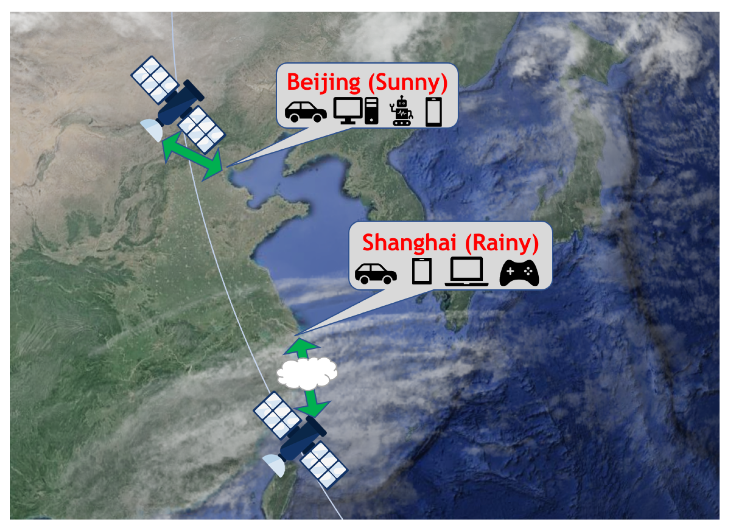
As shown in Figure 1, it is expected that the weather varies from location to location. The satellite over Beijing can choose a coding scheme that can transmit more data because of the clear weather and higher SNR, whereas the satellite over Shanghai can only choose a relatively conservative coding scheme because of the interference from clouds and low SNR. The SNR of the communication link is mainly determined by free-space loss (FSL) and rain loss. However, the current margin value accounting for rain loss is tremendous, which results in the waste of spectrum, so we can dynamically adjust the coding scheme according to the SNR to make full use of the spectrum source.

3.1. Satellite-to-Ground Channel Loss Formulation

We set the scene as terrestrial user equipment (UE) downloading from a satellite. In this scenario, the satellite can dynamically adjust the coding scheme according to the SNR to increase the throughput. The SNR in our scenario is defined as

$$\mathrm{SNR}={EIRP}_{Sat}+{\frac{G}{T}}_{UE}-FSL-k-L_r-B_n-R_b$$

(1)

In this equation, Boltzmann’s constant k is fixed, transmitter power $EIRP$, receiver power $\frac{G}{T}$, and bandwidth $B_n$ are set by the scenario in the beginning and usually remain unchanged. We assume that the transmission rate $R_b$ is constant to observe the band utilization. Here, only the remaining $FSL$ and rain loss $L_r$ are changing.

$$\begin{array}{ccc}\hfill \mathrm{FSL}& =& 20{log}_{10}(\frac{4\pi df}{c})\hfill \end{array}$$

(2)

FSL is only related to distance and frequency, and frequency changes only slightly, so we consider it fixed. Satellites become increasingly closer to us and then fade away, so FSL initially decreases and increases. According to the rain loss calculation method specified by ITU-R P.618-1, rain loss is mainly associated with average rainfall, the altitude, and latitude of UE, elevation angle, and communication frequency. As the communication frequency is fixed, the UE altitude does not easily change, and the elevation angle of each communication is also the same. Therefore, the latitude has the most significant impact. Generally speaking, low-latitude areas have thicker clouds and more significant annual rainfall, while high-latitude areas have lower annual precipitation. Therefore, the rain loss is usually more significant in low-latitude areas, while the rain loss in high-latitude areas is slight. The margin for conventional rain loss, fixed at 6 dB, thus wastes band resources. If we can accurately predict the SNR of the next moment and select a proper coding scheme, band utilization and the throughput can be significantly improved.

Table 1. Abbreviations in the article cross-reference.

Abbreviations	Full Name
AMC	adaptive modulation and coding
AR4JA	accumulate-repeat-4-jagged-accumulate
BER	bit error rate
CCSDS	consultative committee for space data systems
DL	deep learning
DRL	deep reinforce learning
EIRP	equivalent isotropically radiated power
FCC	federal communications commission
FEC	forward error correction
FSL	free-space loss
GAE	generalized advantage estimation
GDP	gross domestic product
G/T	gain-to-noise-temperature
LDPC	low-density parity-check
LEO	low earth orbit
LSTM	long short term memory
MAE	mean absolute error
MDP	markov decision process
PER	package error rate
PPO	proximal policy optimization
QPSK	quadrature phase shift keying
SNR	signal to noise ratio
SVR	support vector regression
SVM	support vector machine
UE	user equipment
UNC	ubiquitous networking and computing

summarizes the terms and their abbreviations in this paper in a cross-reference table.

3.2. AMC Problem Formulation

We assume that the coordinates of a UE are $(lat,lon)$, and the coordinates of a satellite are $(x,y,z)$, and the distance between them can be identified by their coordinates. As cloud thickness and rainfall vary in different locations on Earth, we can use the local real-time weather w and the position of UE $(lat,lon)$ to indicate the local real-time rain loss $L_r$.

$$L_r=g(lat,lon,w)$$

(3)

From Section 3.1, SNR can be expressed as a function of d and $L_r$:

$$\mathrm{SNR}=f(lat,lon,x,y,z,w)$$

(4)

In a real scenario, we do not know the real-time SNR at this moment due to the delay in channel transmission, and for the estimation method normally used, which we denote as $S\widehat{N}R$, we want the error between the estimated value and the true value to be close to 0:

$$|SN{R}_t-S\widehat{N}{R}_t|\stackrel{}{\to }0$$

(5)

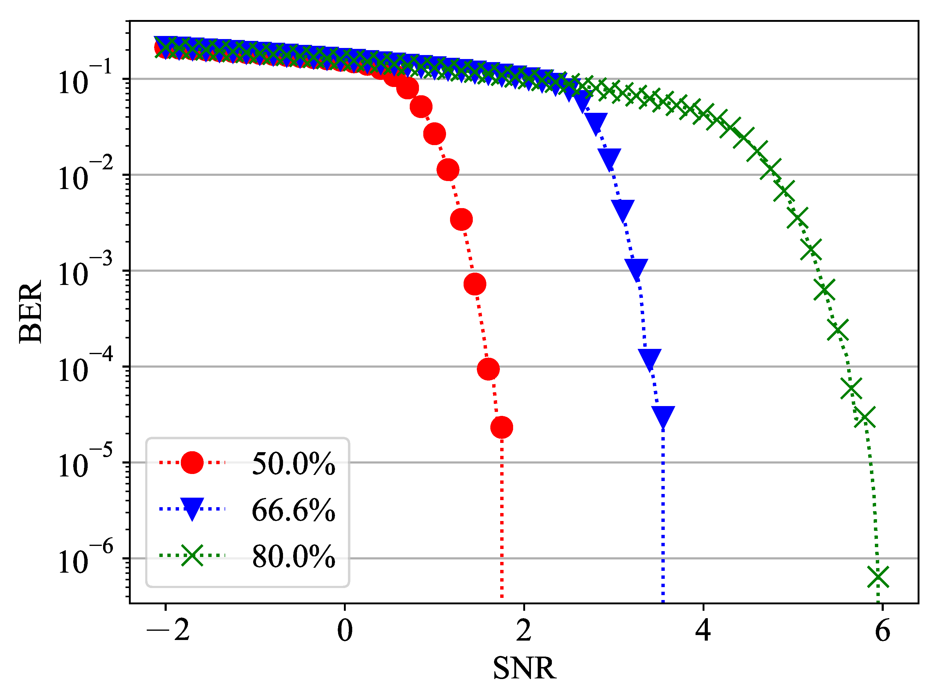
Now that we have obtained an estimate of the real-time SNR, the next task is to select a suitable redundancy rate. The communication coding standard proposed by the consultative committee for space data systems (CCSDS) for use in LEO satellites, uses the accumulate-repeat-4-jagged-accumulate (AR4JA) [37] code was constructed from the protograph based on LDPC, using three data rates of 50%, 66%, and 80%. As is shown in Figure 2, each data rate will have a specific BER at the corresponding SNR. We should try to maximize the data rate while maintaining the quality of communication to obtain the maximum throughput:

$$\underset{DR}{\overset{*}{max}}DR[1-PER(DR,S\widehat{N}R)]$$

(6)

where $DR$ is the data rate and $PER(·)$ represents the package error rate of the corresponding data rate and SNR.

3.3. Markov Decision Process Formulation

As the throughput at this frame is only related to the data rate selected before transmission, we can transform the above problem into an MDP problem represented by a tuple $(\mathcal{S};\mathcal{A};P;r)$, where $\mathcal{S}$ is the set of states observed from the environment, $\mathcal{A}$ is the set of actions from the available selections, the probability distribution of the system is written as $P:\mathcal{S}\times \mathcal{A}\times \mathcal{S}\stackrel{}{\to }\mathcal{R}$, and $r:\mathcal{S}\times \mathcal{A}\times \mathcal{S}\stackrel{}{\to }\mathcal{R}$ is the reward.

We first define the state at time slot t as $s_t$. This part consists of two components: the distance $d_t$ of the satellite-to-ground channel and real-time weather $w_t$. As we can obtain the distance $d_t$ from the satellite position $(x_t,y_t,z_t)$ and the UE position $(la{t}_t,lo{n}_t)$, Moreover, rain loss at different latitudes and longitudes around the world varies. Therefore, we retain the original position information of the state. The connection between the satellite and the UE is concise. Even the longest time is less than 3 min in the Starlink scenario. Hence, we use the weather at the beginning of the connection $w_t$ as the real-time weather for each connection in a single connection. In summary, we define $s_t=\{la{t}_t,lo{n}_t,x_t,y_t,z_t,w_t\}$.

Next, we define the action at time slot t as $a_t=\left\{D{R}_t\right\}$, where $D{R}_t$ is the data rate at time t. It is worth mentioning that the action will not affect the environment itself because the choice of data rate will not affect the location of the satellite and UE, nor will it affect the weather. It will, however, affect the throughput. Although the $BE{R}_t$ will be very low if we choose an overly conservative data rate, the throughput will also be low; on the contrary, selecting an overly aggressive action will cause the receiver to make mistakes, and the $BE{R}_t$ is so high that it cannot communicate normally.

Finally, we define the reward at time t as $r_t=\left\{D{R}_t[1-PER(D{R}_t,SN{R}_t)]\right\}$, where $PER(·)$ represents the package error rate of the corresponding data rate $D{R}_t$ and $SN{R}_t$. In order to transmit more data per time slot, we define $r_t$ as the number of bits transmitted per unit bandwidth. The cumulative reward is $R={\sum }_{t=1}^{\infty }{\gamma }^t{r}_t$, where $\gamma$ is the discount rate.

4. Intelligent Weather-Conscious AMC Scheme for Global Satellite-to-Ground Communications

4.1. Overview

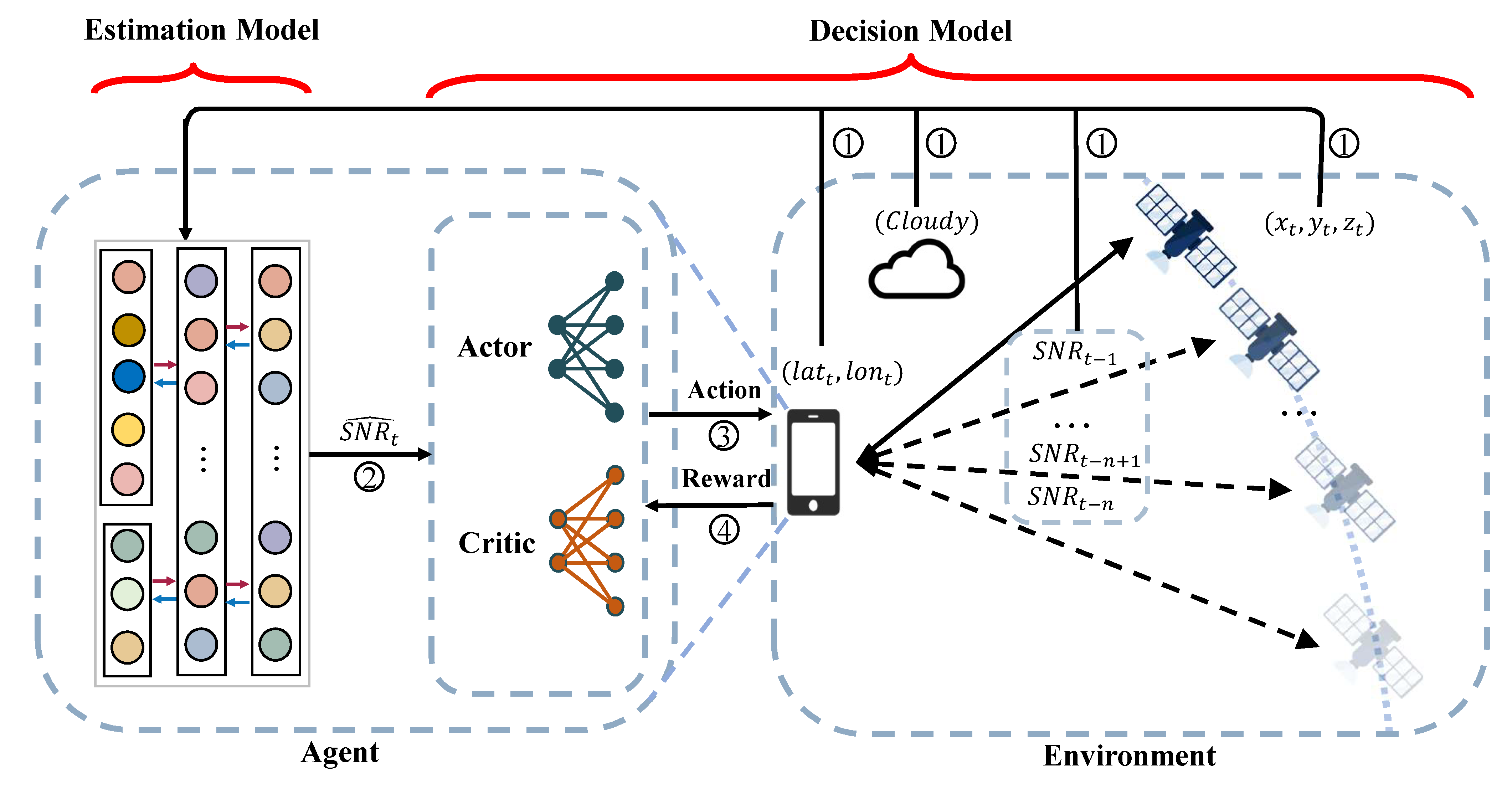
We propose an AMC method for satellite-to-ground based on DL and DRL, which fully considers satellite motion patterns, historical SNRs, and weather conditions. This method can identify transmitter and receiver characteristics, learn online, and adapt to highly variable radio communication scenarios. As shown in Figure 3, the intelligent weather-conscious AMC model processes the position and weather information from the environment. Furthermore, it estimates the state of the satellite-to-ground channel jointly with the past channel information. The coding scheme is then dynamically selected based on the estimation results. So the integrated AMC model can be represented as a DL-based estimation model and a DRL-based decision model. The estimation model makes full use of the historical data of the satellite-to-ground channel and takes the real-time global weather model into account. The decision model can input multi-dimensional information and identify the characteristics of different transmitters and receivers.

First, the estimation model reads information from the environment, including the position of the UE at moment t: $(la{t}_t,lo{n}_t)$, the position of the satellite at moment t: $(x_t,y_t,z_t)$, the SNR for the past moments $\{SN{R}_{t-1},SN{R}_{t-2},\dots ,SN{R}_{t-n}\}$, and the real-time weather conditions. We use one-hot encoding $(Sunny,Cloudy,Rainy)$ to describe weather; if it is currently sunny, the encoding should be $(1,0,0)$, and to write this conveniently, we will use $w_t$ to represent weather at moment t. In summary, the information read by the estimation model from the environment at moment t is $(la{t}_t,lo{n}_t,x_t,y_t,z_t,w_t)$.

Next, when the estimation model predicts the satellite-to-ground channel state at the moment t as $S\widehat{N}{R}_t$, it is passed to the actor-critic network in the decision model to select the optimal encoding scheme. The actor-network is responsible for selecting the optimal encoding scheme, i.e., giving the selected action $a_t$, Moreover, the critic network needs to score the selection of the actor-network, and the two enhance each other and work together to learn the optimal strategy for selecting the encoding. When the actor selects the action $a_t$, it needs to be passed to the environment as the encoding scheme for the satellite-to-ground channel at time t. Finally, the environment will pass back the reward $r_t$, which is the actual throughput $D{R}_t[1-PER(D{R}_t,SN{R}_t)]$ at moment t. This concludes a complete interaction.

4.2. DL-Based Estimation Model

Along with DL development, LSTM is widely used in temporal sequence prediction. Considering that the memorability of LSTM can adequately identify the regular motion of satellites, past SNRs, and weather, we chose the LSTM network as an estimation model to predict the SNR of the next moment.

The input of the LSTM network state $s\left(t\right)$ is divided into two parts: location information and weather information. We classify the global weather into three types: sunny, cloudy, and rainy, and represent them with one-hot encoding $(sunny,cloudy,rainy)$, denote as $w_t$. We denote rainfall and snowfall weather uniformly as rainy because they are both precipitations. The UE on the ground can acquire the weather conditions $w_t$ and its real-time position $(la{t}_t,lo{n}_t)$ and the satellite position for the next moment by storing the satellite orbit information. We use latitude and longitude to describe the location of the UE on the ground. In a practical scenario, we can use GeoHash [38] to compress the latitude and longitude information to 6 bits to reduce the bandwidth consumption while preserving the location information. As satellites have altitude, any 3D coordinate system can, theoretically, describe their position. We use the geographic coordinate system [39] to describe the satellite position, where $(x_t,y_t,z_t)$ denotes the longitude, latitude, and altitude, respectively, of the satellite at the moment t.

After introducing the input for the LSTM network, we introduce its architecture. As shown in Figure 3, the input parameters need to go through the embedding layer first. The embedding layer has two blocks, whereby the first block aims to process weather information and the other block aims to process the location information. Two embedding blocks converge together into an LSTM layer. The LSTM layer, differently from conventional RNNs, controls the flow of information through three gates: the forget, memory, and output gates.

4.2.1. Forget Gate

When new information is input, the model needs to forget some of the old information, and the forget gate is used to select which information to forget and which to keep and, in this way, avoids the problems of gradient disappearance and gradient explosion:

$${\mathbf{f}}_t=\sigma \left[{\mathbf{W}}_{f}s(t-1)+{\mathbf{U}}_f{\mathbf{h}}^{\prime }(t-1)+{\mathbf{b}}_f\right]$$

(7)

where ${\mathbf{W}}_f$ represents the weight between the input and the forget gate, ${\mathbf{U}}_f$ is the weight between the precious hidden state ${\mathbf{h}}^{\prime }(t-1)$ and the forget gate, ${\mathbf{b}}_f$ is the bias of the forget gate, and $\sigma (·)$ is the sigmoid function.

4.2.2. Input Gate

The input gate is used to determine which new information is saved in the cell state of the gate. The input gate is divided into two parts, where one is a control signal consisting of a sigmoid function to control the $\widehat{{\mathbf{C}}_t}$ input, and the other is the estimated cell state $\widehat{{\mathbf{C}}_t}$ at the current moment generated by a $tanh(·)$ function:

$$\begin{array}{cc}\hfill & {\mathbf{i}}_t=\sigma \left[{\mathbf{W}}_{i}s(t-1)+{\mathbf{U}}_i{\mathbf{h}}^{\prime }(t-1)+{\mathbf{b}}_i\right]\hfill \\ \hfill & {\tilde{\mathbf{C}}}_t=tanh\left[{\mathbf{W}}_{c}s(t-1)+{\mathbf{U}}_c{\mathbf{h}}^{\prime }(t-1)+{\mathbf{b}}_c\right]\hfill \end{array}$$

(8)

where ${\mathbf{W}}_i$ and ${\mathbf{W}}_c$ are the weights between the input gate and state $s\left(t\right)$, while ${\mathbf{U}}_i$ and ${\mathbf{U}}_c$ are the weights between the precious hidden layer ${\mathbf{h}}^{\prime }(t-1)$ and the input gate. $tanh(·)$ is a hyperbolic tangent function. The cell state vector is updated as follows:

$${\mathbf{C}}_t={\mathbf{f}}_t\odot \mathbf{C}(t-1)+{\mathbf{i}}_t\odot {\tilde{\mathbf{C}}}_t$$

(9)

where ⊙ represents Hadamard product operator.

4.2.3. Output Gate

The output gate, which is responsible for selectively outputting the hidden state of the cell, has two parts. One is the control signal ${\mathbf{o}}_t$ represented by the sigmoid function, and the other is the final output value ${\mathbf{h}}_t$:

$$\begin{array}{cc}\hfill & {\mathbf{o}}_t=\sigma \left[{\mathbf{W}}_{o}s\left(t\right)+{\mathbf{U}}_o{\mathbf{h}}^{\prime }(t-1)+{\mathbf{b}}_o\right]\hfill \\ \hfill & {\mathbf{h}}^{\prime }\left(t\right)={\mathbf{o}}_t\odot tanh\left({\mathbf{C}}_t\right)\hfill \end{array}$$

(10)

where ${\mathbf{W}}_o$ is the weight between the current input and the output gate and ${\mathbf{U}}_f$ is the weight between the hidden state of the last moment ${\mathbf{h}}^{\prime }(t-1)$ and the output gate. The predicted state is represented as

$$\begin{array}{c}\hfill s_t=\sigma \left[{\mathbf{W}}_t{\mathbf{h}}^{\prime }(t-1)\right]\end{array}$$

(11)

where ${\mathbf{W}}_t$ is the weight vector of the output gate.

The LSTM layer is followed by a fully connected layer, which is used to integrate and analyze the outputs of the LSTM layer. The output layer is connected after the fully connected layer, and since we only need to predict SNR in moment t as $\widehat{SN{R}_t}$, the size of the output layer is one neuron.

The estimation model can be pre-trained using historical information. Finally, the output of the estimation model $\widehat{SN{R}_t}$ is passed to the actor-critic network as input in the decision model. Accurate prediction of the SNR at this moment is crucial, which is the basis upon which the decision model can make correct decisions.

4.3. DRL-Based Decision Model

As MIMO antennas are often used in satellite-to-ground channel communication, the conventional look-up table method cannot cope with it; moreover, in order to be compatible with the gap between different devices and to adapt to the dynamically changing characteristics of the satellite-to-ground channel, we adopt a DRL-based decision model for selecting the optimal coding scheme for each moment.

For simplicity of presentation, we use $s_t,a_t,r_t$ to represent state, action, reward, respectively, at moment t. The state of the decision model is the satellite-to-ground channel state estimated by the estimation model, action is defined as $a_t=\left\{D{R}_t\right\}$, and reward is represented as throughput $r_t=\left\{D{R}_t[1-PER(D{R}_t,SN{R}_t)]\right\}$. We suppose a trajectory exists in the MDP problem and that the trajectory describes the interaction process between the environment and the DRL agent. Therefore, we can obtain the rewards of each time in the trajectory, and the real cumulative reward at state $s_t$ is

$$V^{\prime \pi }\left(s_t\right)=\sum _{\tau =t}^{T\left(\pi \right)}{\gamma }^{\tau -t}{r}_{\tau }$$

(12)

where discount factor $\gamma \in [0,1]$ is a hyperparameter that balances short-term and long-term returns.

There is less accurate data available for learning in satellite-to-ground channel communication, so we want to use historical data fully. Therefore, the Proximal policy optimization (PPO) algorithm [40], based on the actor-critic algorithm [41], is used as the gradient update algorithm. Actor and critic are the two neural networks in the agent. The actor-network is responsible for making decisions and selecting the best action $a_t$, while the critic network is responsible for scoring and evaluating the choice of the actor.

We use this sampled value as the expected cumulative reward to train the critic network. The loss function is defined as

$$\begin{array}{c}\hfill {\mathcal{L}}_c\left(\varphi \right)=\left|\right|V_{\varphi }^{\pi }\left(s_t\right)-V^{\prime \pi }\left(s_t\right){\left|\right|}_2\end{array}$$

(13)

where $\varphi$ is a parameter of the critic network.

The environments of satellite-to-ground channels are similar, under similar environments and similar SNRs, and the choices are likely to be the same. To fully use the information from other trajectories, we introduced importance sampling into gradient propagation.

$$\underset{\theta }{maximize}\widehat{\mathbb{E}}\left[\frac{{\pi }_{\theta }\left(a_t|s_t\right)}{{\pi }_{{\theta }_{\mathrm{old}}}\left(a_t|s_t\right)}\widehat{A}\right]$$

(14)

where ${\pi }_{\theta }\left(a_t\right|s_t)$ is the current policy and ${\pi }_{{\theta }_{old}}\left(a_t\right|s_t)$ is the old policy for collecting trajectory, ${\widehat{A}}_t$ is the estimation of advantage function, which measures how much a specific action $a_t$ is better than the average actions at state $s_t$. To reduce the bias of advantage function, we employ an exponentially weighted method to obtain the Generalized Advantage Estimation (GAE) [42]:

$${\widehat{A}}_t=\sum _{\tau =t}^{T\left(\pi \right)}{\left(\gamma \lambda \right)}^{\tau -t}\left(r_t+\gamma V_{\varphi }^{\pi }\left(s_{t+1}\right)-V^{\prime \pi }\left(s_t\right)\right)$$

(15)

where $\lambda \in [0,1]$ is a hyperparameter. If $t+1>T\left(\pi \right)$, we have $V_{\varphi }^{\pi }\left(s_{t+1}\right)=0$.

Referenced by the gradient descent, we obtain the first-order derivative solution, which is closer to the second-order derivative solution, by adding soft constraints. Due to excessive deviations in the trajectory, we adopted the method in [40] to avoid large gradient deviations.

$${\mathcal{L}}^{\mathcal{CLIP}}(\theta )=\mathbb{E}\left[\sum _{t=0}^T[min(r(\theta ){\widehat{A}}^{{\pi }_k},\mathrm{clip}(r(\theta ),1-ϵ,1+ϵ){\widehat{A}}^{{\pi }_k})]\right]$$

(16)

where $r\left(\theta \right)=\frac{{\pi }_{\theta }\left(a_t\right|s_t)}{{\pi }_{{\theta }_k}\left(a_t\right|s_t)}$ is the ratio between the new policy and the old policy, $ϵ$ is a hyperparameter that denotes the tolerance for the deviation level, and $\mathrm{clip}\left(r\left(\theta \right),1-ϵ,1+ϵ\right)$ modifies the surrogate objective by clipping the probability ratio, which removes the incentive for moving $r(·)$ outside of the interval $[1-ϵ,1+ϵ]$.

Therefore, we can formulate the objective function of the actor network as

$${\mathcal{L}}_a\left(\theta \right)={\mathcal{L}}^{CLIP}\left(\theta \right)+\zeta {\mathbb{E}}_t\left[\mathcal{H}\left({\pi }_{{\theta }_n}\left(a_t\right|s_t)\right)\right]$$

(17)

where $\mathcal{H}\left({\pi }_{{\theta }_n}\left(a_t\right|s_t)\right)$ is an entropy bonus that encourages exploration and $\zeta$ is a balancing hyperparameter. We summarize the training procedure of purposed intelligent weather-conscious AMC in Algorithm 1. Each expectation term is evaluated by the averaged results of a batch of samples.

Algorithm 1:Training of the Intelligent Weather-Conscious AMC.

5. Performance Evaluation

5.1. Simulation Setup

5.1.1. Satellite Constellation

We chose the first phase of SpaceX’s Starlink as the low earth orbit constellation as simulated in the system tool kit (STK), and the scenario of the simulation is shown in Figure 4. Starlink is a constellation of 72 orbits and 22 satellites in each orbit. The inclination of each orbit is 53°, and the satellite’s altitude from the ground is 550 km. As the satellite’s altitude is only 550 km, we can consider that the earth is approximately flat on such a small scale. Using the trigonometric function, we can determine that the satellite can communicate with an area below that can be represented by a circle of radius of 573.5 km. Furthermore, we can find that the satellite can communicate with users whose straight-line distance is as far as $\sqrt{573.5^2+{550}^2}\approx 794.6$ km.

We defined the parameters of the satellite transmitter and receiver according to the technical documents submitted by Starlink to the federal communications commission (FCC) in 2017 [43]; its communication downlink frequency is 10.7–12.7 GHz, transmitter equivalent isotropically radiated power (EIRP) is 10–12.88 dBW/MHz, and receiver power gain-to-noise-temperature (G/T) is 11.1–13.7 dB/K. In our scenario, we take the communication frequency as 12 GHz, EIRP and G/T take the maximum value, EIRP is 12.88 dBW/MHz, and G/T is 13.7 dB/K. After the constellation is fully deployed, the minimum elevation angle is 40 degrees, which means its communication range is determined accordingly. These parameters are also shown in

Table 2. Parameters in the scenario simulation.

Name	Value
Orbit Planes	72
Satellite Per Orbit	22
Inclination	53°
Altitude	550 km
Transmitter EIRP	12.88 dBW/MHz
Receiver G/T	13.7 dB/K
Ground Communication Range Radius	573.5 km
Farthest Connection Distance	794.6 km
Downlink Speed	50 Mbps
Modulation Method	QPSK
Channel Encoding Method	AR4JA
Frequency	12.0 GHz
Data Rate	50%, 66%, 80%
Date	8 and 9 December 2020
Data Interval	1 s

.

5.1.2. Satellite-to-Ground Channel

The influence of clouds and atmosphere needs to be strongly considered in low earth orbit satellite communication scenarios. As stated in Section 3.1, the fading of the satellite-to-ground channel mainly originates from FSL and rain loss, However, to model the realism of the scenario, we also take into account losses such as atmospheric noise, flicker loss, and losses caused by terrain.

After considering the cloud cover and atmospheric environment modeling, we specified the coding approach. We adopted AR4JA as the channel encoding method, with code length $k=1024$ and code rates of 50%, 66%, and 80%. After repeating Monte Carlo simulations 10 million times at different SNRs, we obtain their PER and BER curves, as shown in Figure 2. Quadrature phase-shift keying (QPSK) modulation is adopted as the modulation method. According to users’ actual download speed test nowadays, the maximum is 116 Mbps, so we take 100 Mbps as the downlink speed. In the simulation, we assume that the satellite’s location and the channel quality are derived once per second.

5.1.3. Weather Model

To truly simulate the global communication scenario under different weather conditions, we use hourly weather data from 8 December 2020 to 9 December 2020. We selected 150 cities with the highest gross domestic product (GDP) globally and assumed that users communicate with satellites at these locations. These cities are spread across six continents, and each latitude has a wide range of representation.

As Starlink has an inclination angle of 53°, it cannot communicate with some high-latitude cities (such as Moscow). Finally, 147 cities can communicate with satellites. Due to the fast speed of the satellite, the longest time for each link is about 173 s. Hence, we consider the weather for a single connection to be the weather at the beginning of the connection.

5.1.4. Estimation Model

The estimation model is responsible for processing the information in the environment and predicting the satellite-to-ground channel state. In experiments, we set the satellite-to-ground channel state as SNR. Accurate prediction of SNR with as little introduced noise as possible becomes the keynote of the estimation model network design. In the experiments, we set the LSTM network to contain 100 neurons in 1 layer and set the fully connected layer behind the LSTM layer to also contain 100 neurons as the LSTM network itself is powerful enough.

The neurons responsible for processing weather information and distance information in the embedding layer are $n_W$ and $n_D$, respectively. Their influences on prediction accuracy are discussed in the following text.

The number of passing moments considered by the LSTM network n is also significant. An excessively small n leads the network not fully to consider past information, while an excessively large n will cause the network to consider too much noise, and the training speed and convergence speed will be slow. Thus, we need to strike a balance between the two.

In summary, the network structure of the estimation model from front to back is an embedding layer consisting of $n_W$ and $n_D$ neurons, an LSTM layer containing 100 neurons, a complete connection layer contains 100 neurons, and an output layer contains one neuron.

In the experiment, the learning rate is 0.01, all data are trained at 400 epochs, and the learning rate is reduced at 100 and 200 epochs such that the initial learning rate is multiplied by $0.1$. The sequence length is n, which means that n pieces of data enter the network each time. Therefore, the batch size that we select is 128. We divided the overall dataset into a training set, test set, and validation set according to the ratio of $70\%,$ 20%, and $10\%$. We used STK to collect data from Starlink on 8 December 2020 and the weather data of that day for training, with a total data volume of 600 MB. Mean absolute error (MAE) is served as the criterion of loss. The above parameters are summarized in

Table 3. Parameters in estimation model and decision model.

Name	Value
Neurons in Weather Embedding Layer	$n_W$
Neurons in Distance Embedding Layer	$n_D$
Consider Past Moment Number	n
Estimation Model Learning Rate ${\alpha }_E$	0.01
Estimation Model Training Epochs $E_{max}$	400
Estimation Model Batch Size $b_E$	128
Estimation Model Loss Criterion	MAE
Estimation Model Training Data Set	70%
Estimation Model Validation Data Set	20%
Estimation Model Test Data Set	10%
Decision Model Training Data Set	80%
Decision Model Test Data Set	20%
Decision Model Memory Size $\left|\right|\mathbf{M}\left|\right|$	8192
Decision Model Batch Size $b_D$	2048
Decision Model Repeat Time N	40
Decision Model Maximum Step $S_{max}$	60 k
Decision Model Learning Rate ${\alpha }_D$	0.001
Decision Model Forget Factor $\gamma$	0.3, 0.5, 0.7, 0.9
Baseline (BER) Method Margin	${10}^{-5}$
Baseline (PER) Method Margin	0.1

.

We have chosen the following methods as the estimation methods for comparison:

• Linear Smoothing [17]: The historical data are assigned weights, and the sum of these weights is 1. We define all weights as $\frac{1}{n}$, where n is the number of past moments we need to consider.

  $$\widehat{SN{R}_t}=\sum _{\tau =t-n}^{t-1}\frac{1}{n}SN{R}_{\tau }$$

  (18)
• Exponential Smoothing [17]: Compared to linear smoothing, the importance of the historical data is measured by exponential weights, which focus more on the data at the nearer moments. The sum of the weights is equal to 1.

  $$\widehat{SN{R}_t}=\sum _{\tau =t-n}^{t-1}a{(1-a)}^{t-\tau }SN{R}_{\tau }$$

  (19)

  where a is the weighting factor, and a higher value of a indicates a greater appreciation of historical information. To balance historical and new information, we set a as 0.6.
• SVR [18,19]: SVR borrows ideas from SVM and applies them to the field of time-series prediction.
  Samples that are linearly indistinguishable in low-dimensional space can be linearly distinguishable after mapping to higher dimensions. Kernel function avoids computing the parameters of the nonlinear transformation function and avoids dimensional catastrophe [44]. SVR also adopted this method [45], and the objective function is set as

  $$f\left(x\right)=\sum _{i=0}^{t-1}\left({\widehat{\alpha }}_i-{\alpha }_i\right)\kappa \left(x_i^{T}x\right)+b,$$

  (20)

  where $\widehat{\alpha }$ and $\alpha$ is the Lagrange multiplier, b is the bias term, and $\kappa (·)$ is the kernel function. We adopt the radial basis function [46] as the kernel function.

As the above estimation methods for comparison has a different ability to process information, we provide the linear smoothing and exponential smoothing method with the sequence of past SNRs as input. As SVR cannot, in practice, handle the input mentioned in Section 3.3, we provide SVR with $(d_t,sunny,cloudy,rainy)$ as input, in which the five-dimensional distance information $(la{t}_t,lo{n}_t,x_t,y_t,z_t)$ is processed as distance $d_t$. The disadvantage of this is the loss of the ability to identify different locations around the globe.

5.1.5. Decision Model

The decision model is based on the DRL framework, so we introduce it as two parts: environment and agent.

Environment: The input of the decision model is the output of the estimation model, and the estimation model can achieve high accuracy, so we used accurate SNR data directly in training the decision model. The initial state in the environment is the state at the first moment.

After the agent has selected the action for that step, the environment will step forward accordingly, simulating time change in the real world. We classify 80% of the data as the training set and the other 20% as the test set. We consider one interaction between the satellite and the UE as a trajectory and test the current model performance after collecting one trajectory.

The environment also calculates the throughput based on Equation (6) and returns it to the agent to update its parameters.

Agent: The agent part is mainly composed of the actor and the critic. The neural network structure of actor and critic is $(256,128,64,3)$ neurons in each layer. The activation function between layers is $relu(·)$, and the output layer goes through a $softmax$ function.

The gradient algorithm we adopted is the PPO algorithm mentioned in Algorithm 1, whose memory $\left|\right|\mathbf{M}\left|\right|$ size is 8192, batch size b is 2048, repeat time N is 40 times, and maximum number of steps, $S_{max}$ is 60k. The network parameters are updated every $\left|\right|\mathbf{M}\left|\right|$ step, and the test set data are run once to ensure that the network is not overfitted. The learning rate of both actor and critic networks is $0.001$.

The forgetting factor $\gamma$ is discussed in the following sections, and we discuss the case when $\gamma$ is $(0.3,0.5,0.7,0.9)$ separately. A more prominent forgetting factor means that the system values historical data more, while a smaller forgetting factor means that the system is more straightforward and related to nearby values.

The baseline in the decision model experiment comprises the following.

• Select Data Rate by BER [16]: The BER is the ratio of the erroneous bits to the total number of bits in a frame, and the BER decreases as the SNR increases. The data rate is selected according to BER as the highest data rate among the coding schemes with BER less than ${10}^{-5}$. To simplify writing and drawing, we will hereafter refer to this method as “BER”.
• Select Data Rate by FER [15]: FER is the probability that there is an error code in a frame. FER can be calculated as

  $$FER=1-{(1-BER)}^L$$

  (21)

  where L is the length of a frame.
  FER decreases rapidly as SNR rises. The data rate is selected according to FER as the highest data rate among the coding schemes with FER less than 0.1. To simplify writing and drawing, we will hereafter refer to this method as ”FER”.

To verify the convergence and stability of the algorithm, the experiments were repeated three times for each pair of parameters. To demonstrate the necessity of the estimation model, we also use the state $(la{t}_t,lo{n}_t,x_t,y_t,z_t,w_t)$ in the environment directly in the agent in the experiment, instead of feeding it to its predicted SNR, and the results will be described in Section 5.3.

5.2. Estimation Model Results Analysis

5.2.1. Performance of Different Methods

We adopted the different methods mentioned in Section 5.1.4 as the approach to the estimation model. The results are shown in

Table 4. MAE of Different Methods.

Method	MAE
Linear Smoothing	0.114
Exponential Smoothing	0.062
SVR	0.032
Proposed method	0.014

. So the error can be further reduced, we use MAE as the criterion of the loss function.

Linear smoothing has the worst performance because it takes the average of past moments into account; exponential smoothing has slightly better performance because it favors information from the nearer moments.

The performance of SVR that adopts machine learning methods is excellent. However, LSTM considers the information of past moments, and the MAE is even lower and performs best according to general presence. To show its sustainability, we will discuss the performance of each method in each location around the world in the next part.

5.2.2. Performance in Different Locations

After knowing that LSTM works well in terms of overall performance, we analyze the performance of different methods for different locations. As satellites need to move around the globe, we expect the algorithm to maintain a low MAE and high prediction accuracy at any location. We tested the algorithm’s performance separately for 147 cities around the world. These locations are found on different continents at different latitudes and longitudes and with different weather conditions.

The test results are shown in Figure 5, where the vertical axis is a cumulative distribution function (CDF) plot composed of the test results from different locations around the world. These results indicate that the proposed method performs better than other algorithms in the vast majority of worldwide locations. Even in the worst-performing locations, the MAE of the proposed method is less than 0.07.

5.2.3. Performance According to the Number of Neurons in the Embedding Layer

Different network architectures may lead to the widely varying performance of the network. One of the essential tasks of the estimation model is to interpret weather and distance information in the environment. As mentioned in Section 4.2, different embedding layers are used to handle weather and distance information. We take $n_W$ as the number of neurons in the weather embedding layer and $n_D$ as the number of neurons in the distance embedding layer.

The experimental results are shown in

Table 5. Performance According to Differences in the Number of Neurons in Embedding Layers.

		${\mathit{n}}_{\mathit{W}}$	1	2	3	4	5
	MAE
${\mathit{n}}_{\mathit{D}}$
1			0.93	0.54	0.21	0.029	0.028
2			0.93	0.60	0.20	0.024	0.018
3			0.91	0.61	0.18	0.027	0.014
4			0.90	0.65	0.15	0.06	0.06
5			0.88	0.67	0.12	0.08	0.06

, and it can be seen that the best performance is achieved when $n_W$ and $n_D$ are 3 and 5, respectively. This value corresponds exactly to the number of dimensions of the data in the input states.

5.2.4. Performance of the Number of Past Moments n

LSTM needs to consider information from past moments. Considering too few moments may result in too much focus on current information while ignoring historical information, whereas considering information for excessively long times will introduce more noise. Therefore, we tested the estimation accuracy of the network according to variations in n. The results are shown in

Table 6. MAE of Different Number of Past Moments n.

n	1	2	3	4	5	6	7
MAE	0.06	0.013	0.014	0.016	0.014	0.019	0.019

.

When $n=1$, the LSTM degenerates to a single memory cell with a large MAE. When $n=2$, the LSTM considers the information of the most recent past moments and therefore has the highest accuracy. However, because the network only considers information from very few moments in the past, it is overly reliant on this information and tends to perform poorly in real scenarios with high variability. When $n=3$, the accuracy decreases again, indicating the possibility of overfitting the network at this point, which confirms our conclusion above. As n continues to increase, the MAE also slowly increases. We finally take $n=5$, which not only takes into account the past information more fully but also does not introduce too much noise.

5.3. Decision Model Results Analysis

5.3.1. Necessity of Estimation Model

To demonstrate the importance of the estimation model, we selected the data rate without using the estimation model and used the agent to read the data directly from the environment. The results for when historical information is fully considered, for example, when $\gamma$ is 0.9 or 0.95, are shown in Figure 6. The network can sometimes learn the correct strategy for choosing the data rate, but the variance is enormous and does not ensure the system’s stability. Moreover, the performance is lower than the baseline even after the network converges. Experiments also show that when $\gamma$ is smaller than 0.9, such as when $\gamma$ is 0.5 or 0.7, the training results are a straight line, indicating that the network cannot learn to select a data rate effectively. When $\gamma$ is more significant than 0.95, for example, when $\gamma$ is 0.99, the network fails to learn the correct strategy because it overlooks historical information.

This set of experiments demonstrates that the simple DRL framework is not sufficient to extract useful information from complex states and make choices at the same time. The need for the estimation model is thus confirmed.

5.3.2. Performance of the Forgetting Factor $\gamma$

In this part, we discuss the effect of different $\gamma$ on the results and we conduct experiments for the system performance when $\gamma$ is 0.3, 0.5, 0.7, and 0.9. As shown in Figure 7, the system performs better than the baseline method for different $\gamma$.

An extensive $\gamma$ means paying more attention to historical information, while a small $\gamma$ means paying more attention to current information. The training curves show that the convergence is faster when $\gamma$ is smaller. This indicates that the introduction of the estimation model reduces the difficulty of deciding for the agent and allows it to focus on current information.

Based on the throughput in

Table 7. Throughput of Different Methods.

Method	Throughput
Baseline (BER)	96,316
Baseline (PER)	114,763
Proposed method	118,358

, which is also the reward in the DRL framework, it can be seen that our proposed method improves 22.9% over the BER method and 3.13% over the PER method. We will explore the reasons why performance exceeds the baseline in Section 5.3.3.

5.3.3. Performance According to Different SNRs

To explore the reason for the throughput improvement, we plotted the PER performance of different methods at different SNRs, as shown in Figure 8. When the SNR is very low, the PERs of all methods are high. When the SNR is high, the PERs of the different methods are all 0 and, again, there is no difference.

The “junction” of different encoding schemes, i.e., when the data rate needs to be switched, represents the point at which our method can confer an improvement. To verify the strategy of the proposed method to switch between the adjacent coding schemes, an additional AR4JA code with a code rate of 60% is included in this paper. We have zoomed in on this region in the right half of the figure for ease of observation. The proposed method switches to the following encoding scheme earlier, using a more significant data rate to increase the total throughput. AMC is a trade-off between efficiency and accuracy, and our solution improves total throughput by learning historical information for accurate estimation.

6. Conclusions

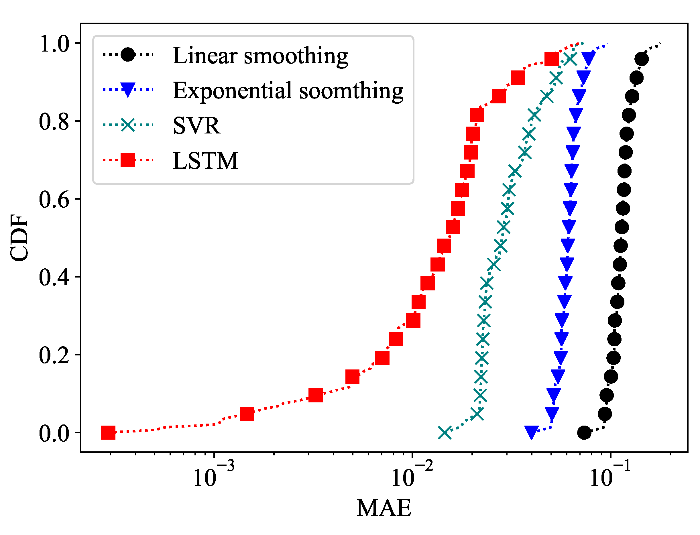
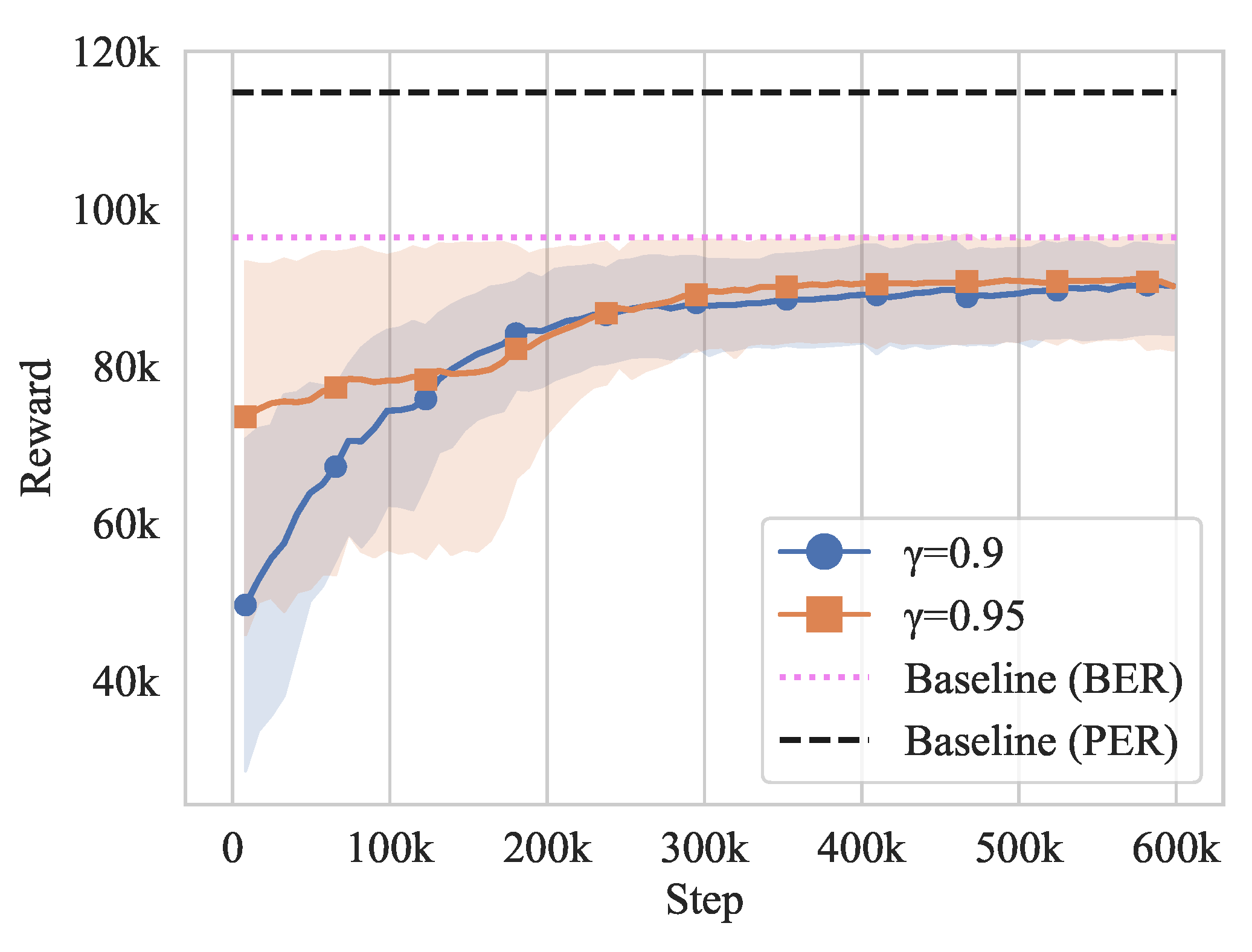
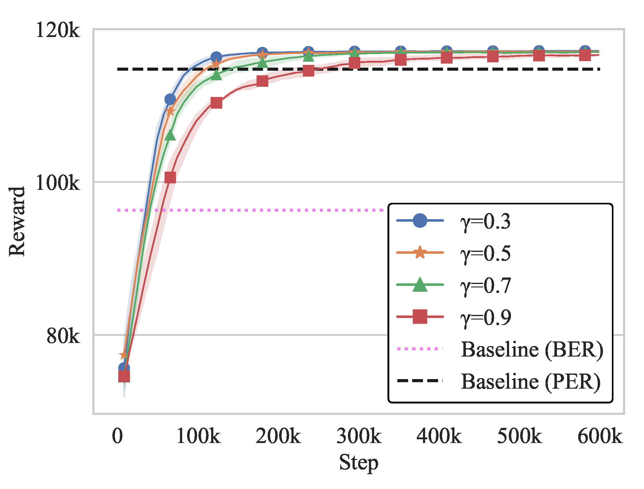
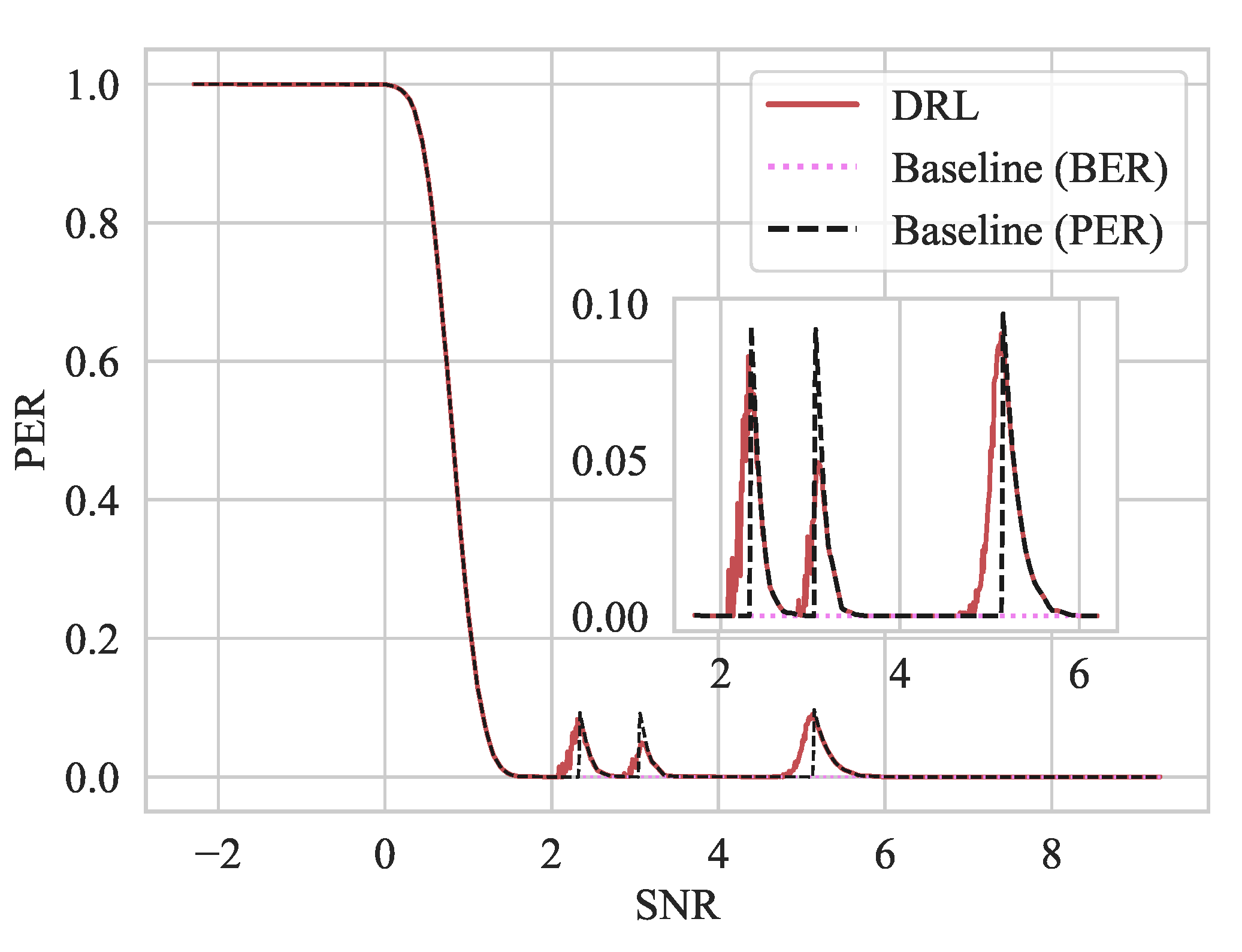
In this paper, we proposed a weather-conscious AMC method for satellite-related UNC. Firstly, the satellite-to-ground scenario was modeled and formulated into an MDP problem. Then, the proposed framework was depicted, which contained the DL-based estimation model and the DRL-based decision model. The estimation model was based on LSTM, which remembered historical information and was responsible for acquiring information from the environment and predicting satellite-to-ground channel states. The decision model was designed based on the actor-critic network. The actor-network in the decision model was responsible for selecting a proper coding method, and the critic network scored the selection of the actor-network. Within our proposed method, the real-time global weather and historical channel information were fully considered, and therefore, the accuracy of channel estimations could be improved. The designed decision model can intelligently switch coding schemes in advance, thus increasing the total throughput of satellite-to-ground communications. Simulations were carried out by using the LSTM network and actor-critic network to verify the performance of the proposed method. Results showed that our estimation model outperformed three existing ones, including SVR, linear soothing, and exponential smoothing. It was also demonstrated that the proposed method improved the throughput by 3.1% over the BER-based and PER-based look-up table method. This work can be helpful to realize the internet connectivity service everywhere in the UNC.