Chipless RFID Sensing System for Precise Ethanol Determination in Alcoholic Solutions

Abstract

The paper presents a new methodology to assess the ethanol content in water solutions. The system exploits a microwave resonator embedded in a polycarbonate sampling cell. The resonator frequency depends on the ethanol percentage and is monitored in real-time through a non-contacting probe. The method shows a precision better than 1% in ethanol percentage in the range of 1–30%, but can be applied also outside this range. Moreover, the methodology can be further improved or adapted for the analysis of other types of aqueous solutions or liquid mixtures upon evaluation of their dielectric properties.

1. Introduction

The development of chipless radio-frequency identification (RFID) technology offers several advantages to the field of radio-frequency (RF) identification. This technology encodes data into the tags by using direct electromagnetic coding into the chipless tag structure instead of embedding silicon chips, which is the usual procedure in conventional RFID systems [1]. This strongly reduces the tag cost, because it opens the way to low-cost mass production of tags, mainly using printing techniques [2,3]. Frequency-encoded chipless RFIDs can be easily adapted and combined with sensing technologies to provide low-cost solutions to a wide range of applications [4,5] including retail, healthcare and pharmaceuticals, food and beverage, precision agriculture, and waste management [4,6,7,8].

The methods that make use of microwave resonators for dielectric analysis are normally divided into resonant and non-resonant categories [9]. Resonant methods are by far more accurate and are especially suited for low-loss materials. Resonant technologies make often use of metamaterials-inspired resonators that have been successfully employed in several dielectric systems operating in the microwave region because of their high Q values and their compactness [10]. Several papers report the determination of the dielectric response of liquids and liquid solutions by using metamaterial-based sensors [11,12,13,14,15]. Only very few of them, however, discuss the intrinsic accuracy of the methodology, which is essential for practical applications.

In this paper, we focused our interest on water-ethanol solutions, because these liquid mixtures are of great interest for the alcoholic beverage industry, and especially for wine quality characterization. Ethanol/water solutions behave as dielectrically homogeneous liquids [16], with no phase separation at any concentration, because of the strong interaction between the ethanol and the water molecules. The most common methods of analysis of ethanol in water-based solutions include High Performance Liquid Chromatography (HPLC) and Near-Infrared Spectroscopy (NIR) [17,18]. Both these techniques are specialized laboratory techniques, and consequently quite expensive. HPLC is very precise, but requires dedicated equipment and trained personnel, standard calibration solutions and is therefore very costly. NIR is less expensive and less precise than HPLC but requires nevertheless a complex sample preparation before analysis. The literature confirms the interest in these solutions, which have been already characterized by dielectric methods by using antennas [11,19] or microstripped resonators [12,20]. Nevertheless, these studies are based on non-resonant technologies and report neither a quantitative estimation of ethanol content nor the intrinsic accuracy and range of applicability of the method, which is of fundamental importance for the practical implementation or the market exploitation. To meet the requirements of the wine industry, the dielectric analysis must be very sensitive to the ethanol content especially when this is low, and consequently, resonant methods are in principle the best approach. The main reason that hinders resonant analysis strategies is the high material loss of both water and ethanol, which makes the achievement of high-Q resonances very difficult, but necessary to make the methodology practically usable in analytical determinations. This paper proposes a novel low-cost method of analysis of liquids based on a chipless RFID sensor structure. This non-contact and real-time monitoring device is designed using a passive microwave resonator embedded in a specifically designed plastic sampling cell. As a simple, cheap, rapid, and non-destructive measuring technique, this method provides information about the dielectric response of liquid materials to electromagnetic fields for specific analysis. It is therefore a convenient method for evaluating food and beverage quality and authenticity. In this work, we analyze the conditions and best frequency range where dielectric resonant analysis can be more efficiently performed, and we propose a simple, fast, and non-contact methodology to determine the ethanol concentration in aqueous solutions with an accuracy of 1% or better making use of only two milliliters of solution and reports a higher sensitivity when compared to similar methods [19,20]. The method uses low-cost materials and could be further optimized, reducing the sensor dimension and therefore the liquid consumption, and can be extended to other liquid/liquid mixtures, provided that the permittivity difference of the components is sufficiently large to have good sensitivity.

2. Frequency Range Analysis and System Design

In order to correctly design the resonant system, it is essential to determine the optimal frequency range where the peaks of the resonator will be best detected, minimizing at the same time the resonator dimension and consequently the liquid consumption. The resonator characteristics have a strong dependence on both its geometrical dimensions and on the dielectric parameters of the medium surrounding it.

The permittivity of a liquid ε is a function of the frequency and is defined as

$$\epsilon ={\epsilon }^{\prime }+j{\epsilon }^{″}$$

(1)

where ε′ and ε″ are its real and imaginary components, respectively. In general, the resonance frequency of a microwave resonator is directly related to its geometrical dimensions. However, a resonating system decreases its peak frequency compared to its value in air when is surrounded by a liquid. This frequency shift is determined only by the real part of the dielectric constant of the liquid. Even though the relationship between ε′ and frequency shift is not linear, the negative shift increases as ε′ increases. However, when the imaginary part of the liquid permittivity ε″ is sensibly different from zero, the resonant peak broadens and when ε″ is sufficiently high, the peak is no longer detectable, and no resonant analysis can be performed. The variation of ε with frequency is usually expressed [16] using the Debye formula.

$${\epsilon }^{\prime }={\epsilon }_{\infty }^{\prime }+\frac{{\epsilon }_{st}^{\prime }-{\epsilon }_{\infty }^{\prime }}{1+{\left(\omega \tau \right)}^2}$$

(2)

$${\epsilon }^{″}=\frac{\left({\epsilon }_{st}^{\prime }-{\epsilon }_{\infty }^{\prime }\right)\omega \tau }{1+{\left(\omega \tau \right)}^2}+\frac{\sigma }{\omega {\epsilon }_0}$$

(3)

where ε₀ is the permittivity of free space, ε_st is the static dielectric constant, and ε_∞ is the ε high-frequency limit. ω = 2πf is the angular frequency and τ is the relaxation time. The effective conductivity, σ, is the ionic conductivity due to dissolved salt or other ions and is negligible for the particular binary system studied in this paper. The dielectric parameters of both water and ethanol follow a simple Debye behavior characterized by a single relaxation time at room temperature and in the range of frequencies going from few MHz to about 10 GHz [16].

As displayed in Figure 1, ε′ of water at 25 °C is stable at 78.5 up to few GHz, while ε′ of ethanol starts decreasing from the low-frequency value of 24.5 at around 400 MHz. On the other hand, while the maximum ε″ value of ethanol is around 10 at 1 GHz, the ε″ value of water keeps increasing with frequency up to 10–12 GHz. To reach the best sensitivity, in principle it is better to choose the range of frequencies where the difference in ε′ is maximum because the shift of the resonance peak mainly depends on this difference. This corresponds approximatively to the range of 2–5 GHz. However, in this range the losses of both water and ethanol are very high, lowering the chances to obtain a clearly detectable resonance peak. On the other hand, in the region around 50–500 MHz, water has a low ε″ value, and the ε′ difference between water and ethanol is high and stable in value. This spectral region can be therefore the most suitable for resonance dielectric analysis, and especially favorable when the ethanol content in the mixture is low because ε″ of water is much lower than that of ethanol.

The resonator was consequently designed to cover this frequency range. The selected design is reported in Figure 2 with all its dimensions. The resonator is square-shaped and includes 6 pairs of interdigitated electrodes (IDE). The use of IDEs is an effective strategy to lower the resonant frequency without increasing the resonator dimensions. The resonator’s lowest resonance was targeted in the range of 300–400 MHz in air.

3. Materials and Methods

The resonator was fabricated by evaporation of 1.1 µm of Aluminum on a 375 µm polycarbonate substrate. After aluminum deposition, the resonator design was transferred on the substrate using photolithographic techniques. The fabricated resonator was then used to realize the sampling cell. The resonator was inserted inside, as reported in Figure 3, in direct contact with the liquid. The cell used for the analytical measurements was built in-house using multiple structured polycarbonate layers bonded together by solvent bonding [21]. The thickness of the liquid layer in the cell was 1.1 mm.

Measurements were performed with an RF-probe directly connected to a VNA (C1220-Copper Mountain Technologies) and the return loss was measured with a sampling interval of 0.2 MHz in the range 10–500 MHz. The distance between the probe and the sampling cell was 16 mm and the probe diameter was 20 mm. The measurements were made by filling the sampling cell with mixtures of water/ethanol at different concentrations in the range 0–100% and measuring the corresponding return loss. The mixtures were prepared using deionized water (from the FBK clean-room deionizing plant) and pure ethanol (Sigma-Aldrich) and the concentrations are calculated as volume ratio. The liquid volume required to fill the cell was 2 mL. The cell was fixed to a plastic support to be held perfectly vertical in a reproducible position after the filling/unfilling procedure. The return loss measured with the probe without sampling cell has been subtracted to all measurements as the baseline.

4. Results and Discussion

The return loss measured with the sampling cell filled with water, ethanol, and selected mixtures of them are shown in Figure 4. Only the 20%, 40%, 60%, and 80% solutions are shown to enhance. As a comparison, also the return loss of the empty cell is reported.

This last curve had to be truncated because is considerably more intense than all the other curves. The lowest frequency peak of the empty cell is centered at 332 MHz, but it moves to 70 MHz and 122 MHz when the cell is filled with water and ethanol, respectively. This huge peak shift is the main characteristic we use for ethanol content determination and is due to the very large relative dielectric constant ε′ of water (78.5) compared to the value of ethanol (24.5) and air (1). On the other hand, the effect of the losses is quite evident. Two peaks are present in the range 50–500 MHz for all pure liquid and mixtures, but the higher frequency peak is broader and less intense, and, in the case of pure ethanol is barely visible. As the frequency and the ethanol content increase, the peak intensity drops dramatically, and, for water-ethanol mixtures at frequencies higher than 400 MHz, the losses become dominant. This means the frequency range 2–5 GHz, where the difference of ε′ between water and ethanol is maximum, is definitely not usable. From Figure 4 it is clear that the shift of the higher frequency peak is more pronounced. This means that in absolute terms the position of this peak is more sensitive to the ethanol content in the mixture, but on the other hand, the peaks are broader and less intense, and the measurement error on the peak position determination is higher. The peak intensity has not been considered in the analysis because it depends on the ethanol percentage in a complex way. Moreover, it is very sensitive to the probe-cell distance and is therefore affected by the positioning error. The peak frequency is quite insensitive to this parameter.

For a more meaningful comparison, we defined the frequency shift Δf as the peak frequency difference between mixture and water and the relative frequency shift Δf/f_water as its fraction of the water peak frequency. In this way, we can compare the frequency variations of the two peaks taking into account the different peak frequency ranges. In this case, as reported in Figure 5, we see that the two peaks overlap perfectly. However, at high ethanol content, only the lower frequency peak is detectable with sufficient precision. The almost perfect overlap is somehow surprising, and it is due to the stability of the ε′ values in the frequency range 50–300 MHz, while the increasing ε″ values in the same range do not affect the peak position. But the most useful information we can obtain from Figure 5 from an analytical perspective is that the data trend is clearly linear in the range 0–30% of ethanol content for both peaks, even though is not linear in all the concentration range investigated. The low ethanol content is the one of greatest interest for the wine and beverages market and considering this we restricted our following analysis to the 0–30% range. Since our purpose is to provide a reliable tool for ethanol content determination, we want to establish what is the detection limit and the intrinsic precision of our methodology. To do this we selected only the data of Figure 5 that fall into the linear region and swapped the x and y-axis to assume that the ethanol percentage is the dependent variable. The data was then fitted assuming a linear dependence of the ethanol content from the relative shift. The formula used for the fit is

y = b·x

(4)

where x is the relative frequency shift and y is the ethanol content. The fit includes only the b parameter because the intercept with the x-axis has been set to zero.

In Figure 6 this linear fit is reported for three different sets of data: the first peak, the second peak, and the combined fit of both peaks. In

Table 1. Statistical parameters for the linear fit of the different data sets displayed in Figure 6.

Data Set	b Value	Standard Error	Relative Standard Error	Person’s r Value
Both peaks	289.3	2.58	0.89%	0.99948
Lower frequency peak	292.5	3.22	1.10%	0.99964
Higher frequency peak	286.2	3.87	1.35%	0.99945
Both peaks without outlier	292.2	2.16	0.73%	0.99967

the basic statistics for the three series of data are reported. The fit results are very similar for the three series, but the combined fit gives the best result in terms of relative error on the b value, which in this case is below 1%. It is also evident that all three series of data can be considered absolutely linear (Pearson’s r value very close to 1) and that the higher frequency peak does not give a more precise determination despite its higher frequency shift.

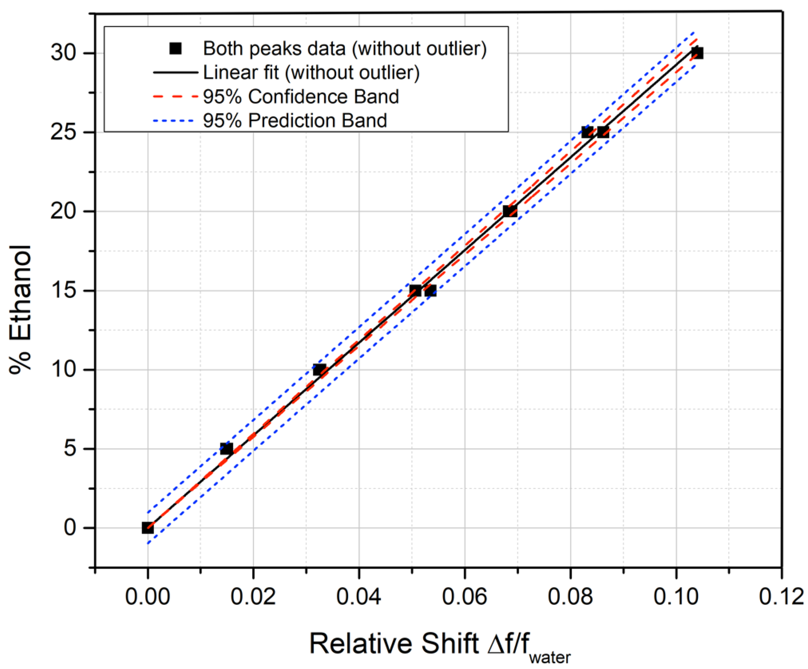
In Figure 7 the residuals are reported for the linear fit of both peaks. All residuals lay within the ±1% of the ethanol concentration, with the only exception of one outlier corresponding to the higher frequency peak of the 30% mixture (red square in Figure 7). This peak is the broadest and least intense peak of the considered interval, and therefore the one with the highest measurement uncertainty. We then decided to remove this point from the data set and rerun the fitting procedure. In this way, the error on the b parameter reduces to 0.73% (Table 1) and the residuals lay within ±0.7% of the fitted ethanol percentage (Figure 7). In Figure 8 the 95% confidence band and prediction band for the ethanol percentage are reported for the fit of both peaks without the outlier. The confidence band is very narrow, and the prediction interval is around ±0.9% of the central value for every concentration.

In

Table 2. Comparison with similar methods for the analysis of water-ethanol solutions.

Frequency for Water (MHz)	Relative Sensitivity 1 (%)	Volume	Range	Reference
4200	0.10%	nL	0–100%	[19]
870	0.09%	mL–µL	0–90%	[20]
70	0.74%	mL	0.100%	This paper
70	0.34%	mL	0–30%	This paper

¹ The relative sensitivity is the ratio between the sensitivity and the peak frequency with pure water, corresponding to the relative shift Δf/f_water for the variation of 1% of ethanol content.

, a comparison with similar methods reported in the references has been reported. To be consistent with data reported in Figure 5, Figure 6 and Figure 8, and to compare systems working at different frequencies, the sensitivity in MHz/% has been divided by the resonant frequency measured with pure water, resulting in the relative shift Δf/f_water for 1% variation of ethanol content. The methodology of this paper is by far the most sensitive in terms of relative frequency shift when compared to the others, and the only one that reports the precision of the methodology employed. However, the sample quantity required for the analysis is larger than in the other cases, and this can be a direction where our system can be improved.

Our methodology can therefore be used to determine the ethanol content in solution with an error below 1%, and, with further refinement and calibration optimization, this limit can be lowered considerably. However, it should be mentioned that the typical alcoholic beverage is not a simple mixture of water and ethanol but a more complex liquid. When applied to a specific product, this limit should be verified, because interferences from other components may be important. Moreover, this determination does not consider the effect of temperature variations on the dielectric parameters. If the temperature is sensibly different from standard ambient temperature, this effect can be compensated with a calibration using pure water or pure ethanol before the analysis.

5. Conclusions and Outlook

We demonstrated that the methodology proposed is able to detect the ethanol content with precision around or better than 1% but this parameter can be improved in different ways, and this will be the focus of our future work. Using more water-ethanol solutions of different concentrations will improve the number of data points and the calibration curve precision. Consequently, the error on the b parameter and the prediction intervals can be strongly reduced. In addition, an optimization of the design of the whole system, including the Q-factor of the resonator, the thickness of the liquid in the cell, the reading distance, and the precision of the cell positioning can further reduce the measurement error by at least an order of magnitude. The resonator dimensions and quantity of liquid used for the analysis can be minimized with an optimization of the resonator and cell design. Moreover, other concentration ranges outside the 0–30% of ethanol can be assessed using a non-linear fitting function (e.g., quadratic). Even though the linear dependence has some obvious advantages, the relative shift is higher at high ethanol percentages than in the 0–30% range, making the detection methodology more sensitive. Lastly, the proposed detection system can be easily adapted to analyze liquid solutions with different liquid components, rescaling the optimal resonator dimensions and frequency range depending on the dielectric parameters of the specific liquids. However, the applicability to other liquid solutions depends on the difference on the permittivity values of the liquids involved because this is directly related to the sensitivity. Liquid with similar permittivity cannot be distinguished with this method. Lastly, but importantly, the method will be tested on real alcoholic beverages, such as beer or wine to verify its applicability and reliability to real consumer products.