
Enhanced Credit Card Fraud Detection Model Using Machine Learning


Abstract
:1. Introduction
2. Related Work
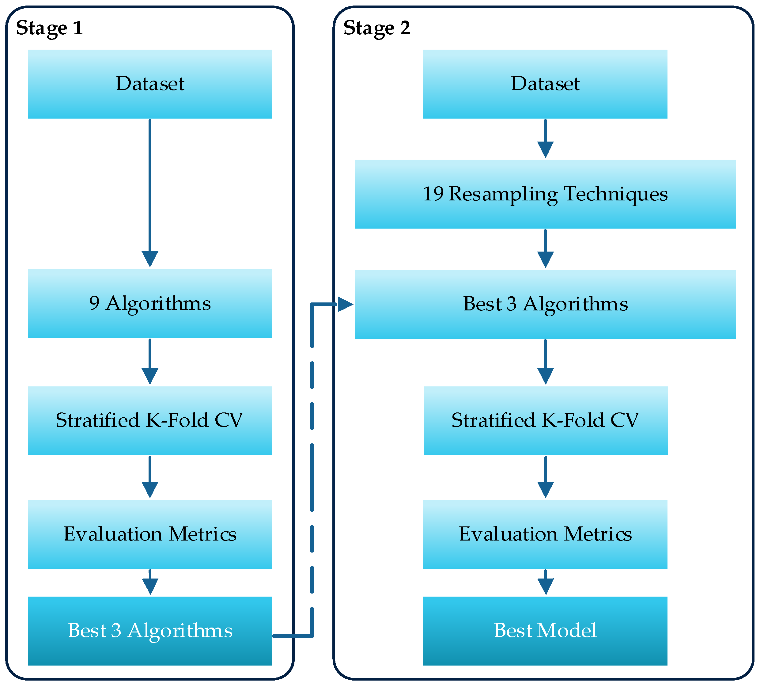
3. Proposed Approach
3.1. Simulation Environment
3.1.1. Software
3.1.2. Hardware
- Processor: Intel(R) Xeon(R) CPU D-1527 @ 2.20 GHz 2.19 GHz.
- RAM: 7.00 GB.
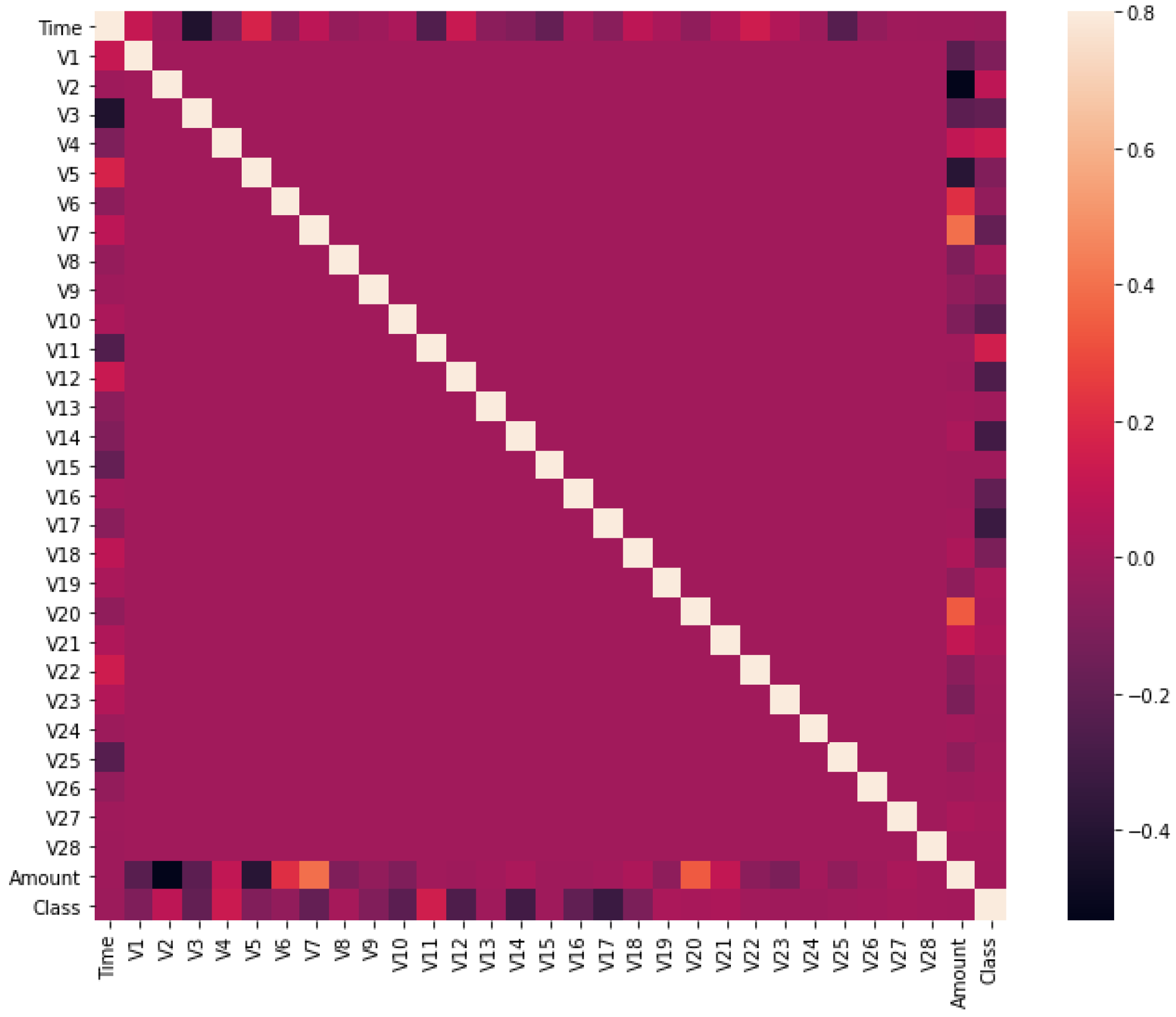
3.2. Dataset
3.3. Algorithms
3.3.1. Logistic Regression
3.3.2. K-Nearest Neighbors
3.3.3. Decision Tree
3.3.4. CatBoost
3.3.5. XGBoost
3.3.6. GBM
3.3.7. LightGBM
3.3.8. Naïve Bayes
3.3.9. Random Forest
3.4. Resampling Techniques
3.4.1. Undersampling
3.4.2. Oversampling
3.4.3. Combination of Both Undersampling and Oversampling
3.4.4. The 19 Resampling Techniques
- Eleven undersampling techniques.
- Six oversampling techniques.
- Two combinations of both undersampling and oversampling techniques at once.
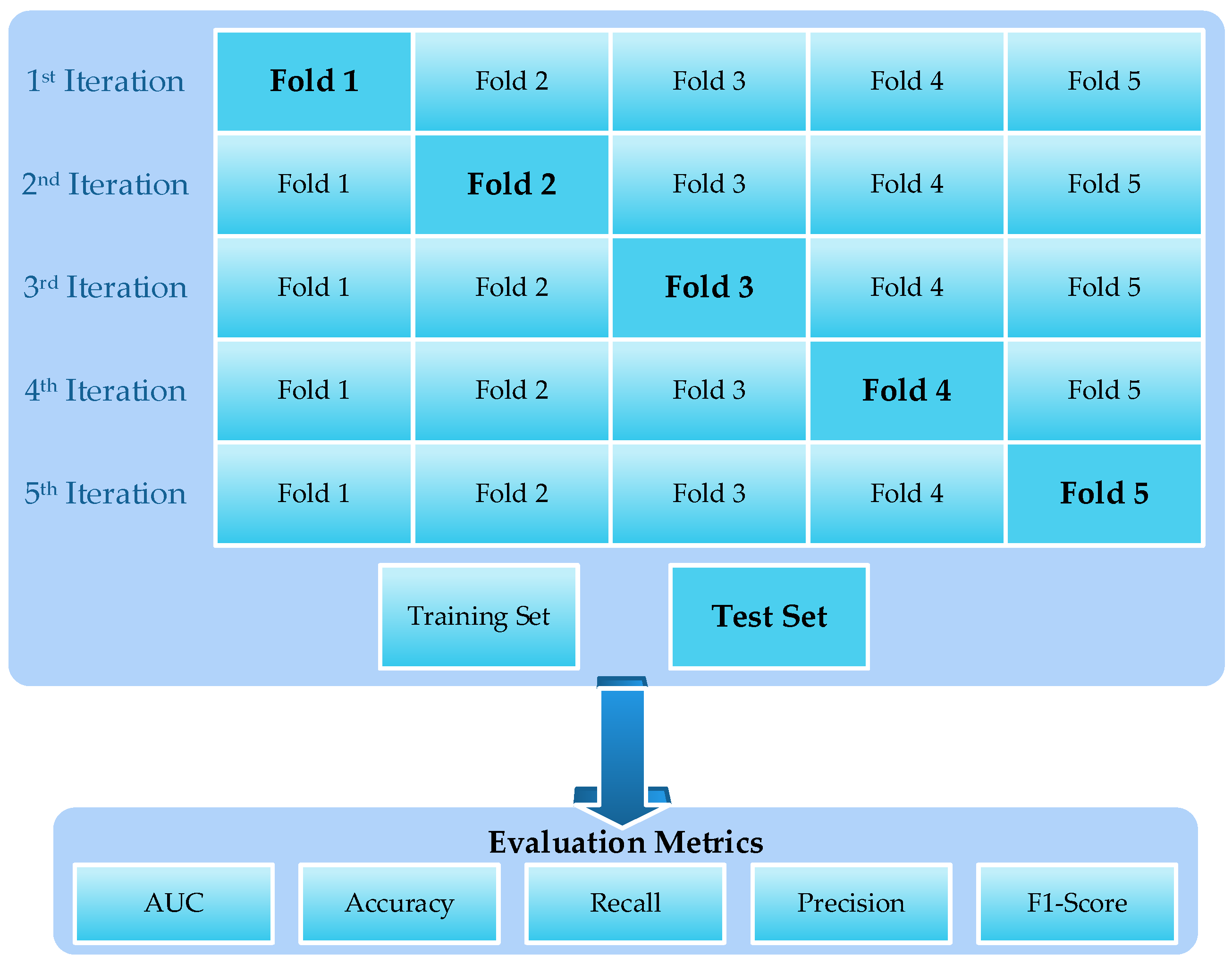
3.5. Stratified K-Fold Cross-Validation
3.6. Evaluation Metrics
4. Results
4.1. The First Stage: Algorithm Comparison
4.2. The Second Stage: Resampling Techniques
4.2.1. AUC
4.2.2. Accuracy
4.2.3. Recall
4.2.4. Precision
4.2.5. F1-Score
4.3. Comparison with Previous Works
5. Conclusions and Future Work
Author Contributions
Funding
Conflicts of Interest
References
- Dubey, S.C.; Mundhe, K.S.; Kadam, A.A. Credit Card Fraud Detection using Artificial Neural Network and BackPropagation. In Proceedings of the 2020 4th International Conference on Intelligent Computing and Control Systems (ICICCS), Rasayani, India, 13–15 May 2020; pp. 268–273. [Google Scholar] [CrossRef]
- Martin, T. Credit Card Fraud: The Biggest Card Frauds in History. Available online: https://www.uswitch.com/credit-cards/guides/credit-card-fraud-the-biggest-card-frauds-in-history/ (accessed on 22 January 2022).
- Zhang, X.; Han, Y.; Xu, W.; Wang, Q. HOBA: A novel feature engineering methodology for credit card fraud detection with a deep learning architecture. Inf. Sci. 2019, 557, 302–316. [Google Scholar] [CrossRef]
- Makki, S.; Assaghir, Z.; Taher, Y.; Haque, R.; Hacid, M.-S.; Zeineddine, H. An experimental study with imbalanced classification approaches for credit card fraud detection. IEEE Access 2019, 7, 93010–93022. [Google Scholar] [CrossRef]
- McCue, C. Advanced Topics. Data Mining and Predictive Analysis; Butterworth-Heinemann: Oxford, UK, 2015; pp. 349–365. [Google Scholar]
- Berad, P.; Parihar, S.; Lakhani, Z.; Kshirsagar, A.; Chaudhari, A. A Comparative Study: Credit Card Fraud Detection Using Machine Learning. J. Crit. Rev. 2020, 7, 1005. [Google Scholar]
- Jain, Y.; Namrata, T.; Shripriya, D.; Jain, S. A comparative analysis of various credit card fraud detection techniques. Int. J. Recent Technol. Eng. 2019, 7, 402–403. [Google Scholar]
- Tolles, J.; Meurer, W.J. Logistic regression: Relating patient characteristics to outcomes. JAMA 2016, 316, 533–534. [Google Scholar] [CrossRef] [PubMed]
- Shirodkar, N.; Mandrekar, P.; Mandrekar, R.S.; Sakhalkar, R.; Kumar, K.C.; Aswale, S. Credit card fraud detection techniques–A survey. In Proceedings of the 2020 International Conference on Emerging Trends in Information Technology and Engineering (ic-ETITE), Shiroda, India, 13–15 May 2020; pp. 1–7. [Google Scholar] [CrossRef]
- Gaikwad, J.R.; Deshmane, A.B.; Somavanshi, H.V.; Patil, S.V.; Badgujar, R.A. Credit Card Fraud Detection using Decision Tree Induction Algorithm. Int. J. Innov. Technol. Explor. Eng. IJITEE 2014, 4, 66–67. [Google Scholar]
- Zareapoor, M.; Seeja, K.; Alam, M.A. Analysis on credit card fraud detection techniques: Based on certain design criteria. Int. J. Comput. Appl. 2012, 52, 35–42. [Google Scholar] [CrossRef]
- Friedman, J.H. Greedy function approximation: A gradient boosting machine. Ann. Stat. 2001, 29, 1189–1232. [Google Scholar] [CrossRef]
- Microsoft. LightGBM. Available online: https://github.com/microsoft/LightGBM (accessed on 22 January 2021).
- XGBoost Developers. Introduction to Boosted Trees. Available online: https://xgboost.readthedocs.io/en/latest/tutorials/model.html (accessed on 22 January 2022).
- Yandex Technologies. CatBoost. Available online: https://yandex.com/dev/catboost/ (accessed on 22 January 2022).
- Delamaire, L.; Abdou, H.; Pointon, J. Credit card fraud and detection techniques: A review. Banks Bank Syst. 2009, 4, 61. [Google Scholar]
- Khatri, S.; Arora, A.; Agrawal, A.P. Supervised machine learning algorithms for credit card fraud detection: A comparison. In Proceedings of the 2020 10th International Conference on Cloud Computing, Data Science & Engineering (Confluence), Noida, India, 29–31 January 2020; pp. 680–683. [Google Scholar] [CrossRef]
- Taha, A.A.; Malebary, S.J. An intelligent approach to credit card fraud detection using an optimized light gradient boosting machine. IEEE Access 2020, 8, 25579–25587. [Google Scholar] [CrossRef]
- Vengatesan, K.; Kumar, A.; Yuvraj, S.; Kumar, V.; Sabnis, S. Credit card fraud detection using data analytic techniques. Adv. Math. Sci. J. 2020, 9, 1185–1196. [Google Scholar] [CrossRef]
- Puh, M.; Brkić, L. Detecting credit card fraud using selected machine learning algorithms. In Proceedings of the 2019 42nd International Convention on Information and Communication Technology, Electronics and Microelectronics (MIPRO), Zagreb, Croatia, 20–24 May 2019; pp. 1250–1255. [Google Scholar] [CrossRef]
- Hema, A. Machine Learning methods for Discovering Credit Card Fraud. Int. Res. J. Comput. Sci. 2020, 8, 1–6. [Google Scholar]
- Kumar, M.S.; Soundarya, V.; Kavitha, S.; Keerthika, E.; Aswini, E. Credit card fraud detection using random forest algorithm. In Proceedings of the 2019 3rd International Conference on Computing and Communications Technologies (ICCCT), Chennai, India, 21–22 February 2019; pp. 149–153. [Google Scholar] [CrossRef]
- Patidar, R.; Sharma, L. Credit card fraud detection using neural network. Int. J. Soft Comput. Eng. IJSCE 2011, 1, 32–38. [Google Scholar]
- Asha, R.; KR, S.K. Credit card fraud detection using artificial neural network. Glob. Trans. Proc. 2021, 2, 35–41. [Google Scholar] [CrossRef]
- Varmedja, D.; Karanovic, M.; Sladojevic, S.; Arsenovic, M.; Anderla, A. Credit card fraud detection-machine learning methods. In Proceedings of the 2019 18th International Symposium Infoteh-Jahorina (Infoteh), Novi Sad, Serbia, 20–22 March 2019; pp. 1–5. [Google Scholar] [CrossRef]
- Breunig, M.M.; Kriegel, H.P.; Ng, R.T.; Sander, J. LOF: Identifying density-based local outliers. In Proceedings of the 2000 ACM SIGMOD International Conference on Management of Data, Dallas, TX, USA, 15–18 May 2000; pp. 93–104. [Google Scholar] [CrossRef]
- Liu, F.T.; Ting, K.M.; Zhou, Z.H. Isolation forest. In Proceedings of the 2008 Eighth IEEE International Conference on Data Mining, Ballarat, VIC, Australia, 15–19 December 2008; pp. 413–422. [Google Scholar] [CrossRef]
- John, H.; Naaz, S. Credit card fraud detection using local outlier factor and isolation forest. Int. J. Comput. Sci. Eng 2019, 7, 1060–1064. [Google Scholar] [CrossRef]
- Dal Pozzolo, A.; Caelen, O.; Johnson, R.A.; Bontempi, G. Calibrating probability with undersampling for unbalanced classification. In Proceedings of the 2015 IEEE Symposium Series on Computational Intelligence, Cape Town, South Africa, 7–10 December 2015; pp. 159–166. [Google Scholar] [CrossRef]
- Sahin, Y.; Duman, E. Detecting credit card fraud by ANN and logistic regression. In Proceedings of the 2011 International Symposium on Innovations in Intelligent Systems and Applications, Istanbul, Turkey, 15–18 June 2011; pp. 315–319. [Google Scholar]
- Kokkinaki, A.I. On atypical database transactions: Identification of probable frauds using machine learning for user profiling. In Proceedings of the 1997 IEEE Knowledge and Data Engineering Exchange Workshop, Nicosia, Cyprus, 4 November 1997; p. 109. [Google Scholar]
- Piryonesi, S.M.; El-Diraby, T.E. Data analytics in asset management: Cost-effective prediction of the pavement condition index. J. Infrastruct. Syst. 2020, 26, 04019036. [Google Scholar] [CrossRef]
- Maes, S.; Tuyls, K.; Vanschoenwinkel, B.; Manderick, B. Credit card fraud detection using Bayesian and neural networks. In Proceedings of the 1st International Naiso Congress on Neuro Fuzzy Technologies, Brussel, Belgium, 16–19 January 2002; pp. 261–270. [Google Scholar]
- Syeda, M.; Zhang, Y.Q.; Pan, Y. Parallel granular neural networks for fast credit card fraud detection. In Proceedings of the 2002 IEEE World Congress on Computational Intelligence. 2002 IEEE International Conference on Fuzzy Systems. FUZZ-IEEE’02. Proceedings (Cat. No. 02CH37291), Atlanta, GA, USA, 12–17 May 2002; pp. 572–577. [Google Scholar] [CrossRef]
- Seeja, K.; Zareapoor, M. Fraudminer: A novel credit card fraud detection model based on frequent itemset mining. Sci. World J. 2014, 2014, 1–10. [Google Scholar] [CrossRef]
- Scikit-Learn-Contrib. Imbalanced-Learn. Available online: https://github.com/scikit-learn-contrib/imbalanced-learn (accessed on 22 January 2022).
- He, H.; Garcia, E.A. Learning from imbalanced data. IEEE Trans. Knowl. Data Eng. 2009, 21, 1263–1284. [Google Scholar] [CrossRef]
- Dal Pozzolo, A.; Caelen, O.; Bontempi, G. When is undersampling effective in unbalanced classification tasks? In Proceedings of the Joint European Conference on Machine Learning and Knowledge Discovery in Databases, Porto, Portugal, 7–11 September 2015; pp. 200–215. [Google Scholar]
- García, V.; Mollineda, R.A.; Sánchez, J.S. On the k-NN performance in a challenging scenario of imbalance and overlapping. Pattern Anal. Appl. 2008, 11, 269–280. [Google Scholar] [CrossRef]
- Cieslak, D.A.; Chawla, N.V. Start globally, optimize locally, predict globally: Improving performance on imbalanced data. In Proceedings of the 2008 Eighth IEEE International Conference on Data Mining, Notre Dame, IN, USA, 15–19 December 2008; pp. 143–152. [Google Scholar]
- Scikit-Learn Developers. 3.1. Cross-validation: Evaluating Estimator Performance. Available online: https://scikit-learn.org/stable/modules/cross_validation.html (accessed on 22 January 2022).
- Hanley, J.A.; McNeil, B.J. The meaning and use of the area under a receiver operating characteristic (ROC) curve. Radiology 1982, 143, 29. [Google Scholar] [CrossRef] [Green Version]
- Stehman, S.V. Selecting and interpreting measures of thematic classification accuracy. Remote Sens. Environ. 1997, 62, 77. [Google Scholar] [CrossRef]
- Fawcett, T. An introduction to ROC analysis. Pattern Recognit. Lett. 2006, 27, 862. [Google Scholar] [CrossRef]
- Powers, D.M. Evaluation: From precision, recall and F-measure to ROC, informedness, markedness and correlation. arXiv 2020, arXiv:2010.16061. [Google Scholar]
- Chicco, D.; Tötsch, N.; Jurman, G. The Matthews correlation coefficient (MCC) is more reliable than balanced accuracy, bookmaker informedness, and markedness in two-class confusion matrix evaluation. BioData Min. 2021, 14, 1–22. [Google Scholar] [CrossRef] [PubMed]
- Google Developers. Classification: ROC Curve and AUC. Available online: https://developers.google.com/machine-learning/crash-course/classification/roc-and-auc (accessed on 22 January 2022).
- DeepAI. Accuracy (Error Rate). Available online: https://deepai.org/machine-learning-glossary-and-terms/accuracy-error-rate (accessed on 22 January 2022).
- Guido, S.; Müller, A.C. Introduction to Machine Learning with Python A Guide for Data Scientists; O’Reilly: Sebastopol, CA, USA, 2021; p. 282. [Google Scholar]
- C3, AI. Precision. Available online: https://c3.ai/glossary/machine-learning/precision/ (accessed on 22 January 2022).
- Masís, S. Interpretable Machine Learning with Python: Learn to Build Interpretable High-Performance Models with Hands-On Real-World Examples; Packt Publishing Ltd.: Birmingham, UK, 2021; p. 81. [Google Scholar]
- Prusti, D.; Rath, S.K. Fraudulent transaction detection in credit card by applying ensemble machine learning techniques. In Proceedings of the 2019 10th International Conference on Computing, Communication and Networking Technologies (ICCCNT), Rourkela, India, 6–8 July 2019; pp. 1–6. [Google Scholar] [CrossRef]
- Wang, G.-G.; Deb, S.; Cui, Z. Monarch butterfly optimization. Neural Comput. Appl. 2019, 31, 1995–2014. [Google Scholar] [CrossRef] [Green Version]
- Ghosh, I.; Roy, P.K. Application of earthworm optimization algorithm for solution of optimal power flow. In Proceedings of the 2019 International Conference on Opto-Electronics and Applied Optics (Optronix), Kolkata, India, 18–20 March 2019; pp. 1–6. [Google Scholar] [CrossRef]
- Wang, G.-G.; Deb, S.; Coelho, L.d.S. Elephant herding optimization. In Proceedings of the 2015 3rd International Symposium on Computational and Business Intelligence (ISCBI), Xuzhou, China, 7–9 December 2015; pp. 1–5. [Google Scholar] [CrossRef]
- Wang, G.-G. Moth search algorithm: A bio-inspired metaheuristic algorithm for global optimization problems. Memetic Comput. 2018, 10, 151–164. [Google Scholar] [CrossRef]
- Heidari, A.A.; Mirjalili, S.; Faris, H.; Aljarah, I.; Mafarja, M.; Chen, H. Harris hawks optimization: Algorithm and applications. Future Gener. Comput. Syst. 2019, 97, 849–872. [Google Scholar] [CrossRef]


| Type | Technique | Abbreviation |
|---|---|---|
| Undersampling | Random Undersampling | RUS |
| Condensed Nearest Neighbor | CNN | |
| Tomek | Tomek | |
| One-Sided Selection | OSS | |
| Edited Nearest Neighbors | ENN | |
| Repeated Edited Nearest Neighbors | RENN | |
| All K-Nearest Neighbors | AllKNN | |
| Neighborhood Cleaning Rule | NCR | |
| Near Miss 1 | NM1 | |
| Near Miss 2 | NM2 | |
| Instance Hardness Threshold | IHT | |
| Oversampling | Random Oversampling | ROS |
| Synthetic Minority Oversampling Technique | SMOTE | |
| Adaptive Synthetic | ADASYN | |
| Borderline SMOTE 1 | Border1 | |
| Borderline SMOTE 2 | Border2 | |
| SVM SMOTE | SVMSM | |
| Both Undersampling and Oversampling | SMOTEENN | SMENN |
| SMOTETomek | SMTomek |
| Classifier | AUC | Accuracy | Recall | Precision | F1-Score |
|---|---|---|---|---|---|
| LR | 0.8483 | 0.9989 | 0.6971 | 0.6462 | 0.6688 |
| KNN | 0.9180 | 0.9984 | 0.8375 | 0.0956 | 0.1711 |
| DT | 0.8722 | 0.9991 | 0.7449 | 0.7724 | 0.7581 |
| NB | 0.5736 | 0.9929 | 0.1478 | 0.6485 | 0.2405 |
| RF | 0.9742 | 0.9996 | 0.9487 | 0.7846 | 0.8588 |
| GBM | 0.8841 | 0.9990 | 0.7688 | 0.6034 | 0.6615 |
| LightGBM | 0.6246 | 0.9959 | 0.2499 | 0.5612 | 0.3410 |
| XGBoost | 0.9760 | 0.9996 | 0.9523 | 0.8008 | 0.8698 |
| Catboost | 0.9804 | 0.9996 | 0.9612 | 0.7967 | 0.8711 |
| Technique | AUC | Accuracy | Recall | Precision | F1-Score |
|---|---|---|---|---|---|
| Without | 0.9804 | 0.9996 | 0.9612 | 0.7967 | 0.8711 |
| RUS | 0.5331 | 0.9776 | 0.0663 | 0.9065 | 0.1234 |
| CNN | 0.7496 | 0.9982 | 0.4994 | 0.8597 | 0.6306 |
| Tomek | 0.9768 | 0.9996 | 0.9539 | 0.7947 | 0.8670 |
| OSS | 0.9806 | 0.9996 | 0.9616 | 0.7948 | 0.8699 |
| ENN | 0.9791 | 0.9996 | 0.9586 | 0.7947 | 0.8689 |
| RENN | 0.9782 | 0.9996 | 0.9568 | 0.8029 | 0.8730 |
| AllKNN | 0.9794 | 0.9996 | 0.9591 | 0.8028 | 0.8740 |
| NCR | 0.9792 | 0.9996 | 0.9587 | 0.7967 | 0.8702 |
| NM1 | 0.5037 | 0.7698 | 0.0075 | 0.9350 | 0.0149 |
| NM2 | 0.5005 | 0.0160 | 0.0017 | 0.9939 | 0.0035 |
| IHT | 0.5007 | 0.0300 | 0.0018 | 0.9939 | 0.0035 |
| ROS | 0.9045 | 0.9994 | 0.8093 | 0.8435 | 0.8256 |
| SMOTE | 0.8627 | 0.9992 | 0.7256 | 0.8476 | 0.7811 |
| ADASYN | 0.8327 | 0.9990 | 0.6657 | 0.8435 | 0.7431 |
| Border1 | 0.9139 | 0.9994 | 0.8281 | 0.8231 | 0.8253 |
| Border2 | 0.8869 | 0.9993 | 0.7741 | 0.8313 | 0.8014 |
| SVMSM | 0.9291 | 0.9995 | 0.8585 | 0.8231 | 0.8403 |
| SMENN | 0.8486 | 0.9991 | 0.6975 | 0.8414 | 0.7617 |
| SMTomek | 0.8295 | 0.9990 | 0.6593 | 0.8435 | 0.7400 |
| Technique | AUC | Accuracy | Recall | Precision | F1-Score |
|---|---|---|---|---|---|
| Without | 0.9760 | 0.9996 | 0.9523 | 0.8008 | 0.8698 |
| RUS | 0.5210 | 0.9638 | 0.0422 | 0.9146 | 0.0806 |
| CNN | 0.7058 | 0.9976 | 0.4119 | 0.8638 | 0.5558 |
| Tomek | 0.9748 | 0.9996 | 0.9499 | 0.8008 | 0.8689 |
| OSS | 0.9769 | 0.9996 | 0.9541 | 0.7947 | 0.8669 |
| ENN | 0.9727 | 0.9996 | 0.9457 | 0.8049 | 0.8695 |
| RENN | 0.9737 | 0.9996 | 0.9477 | 0.8029 | 0.8692 |
| AllKNN | 0.9725 | 0.9996 | 0.9453 | 0.8008 | 0.8670 |
| NCR | 0.9714 | 0.9996 | 0.9431 | 0.8009 | 0.8659 |
| NM1 | 0.5026 | 0.6754 | 0.0054 | 0.9472 | 0.0107 |
| NM2 | 0.5004 | 0.0105 | 0.0017 | 0.9959 | 0.0035 |
| IHT | 0.5008 | 0.0413 | 0.0018 | 0.9939 | 0.0036 |
| ROS | 0.9598 | 0.9996 | 0.9200 | 0.8252 | 0.8697 |
| SMOTE | 0.9306 | 0.9995 | 0.8614 | 0.8394 | 0.8501 |
| ADASYN | 0.9203 | 0.9995 | 0.8408 | 0.8435 | 0.8420 |
| Border1 | 0.9647 | 0.9996 | 0.9298 | 0.8231 | 0.8730 |
| Border2 | 0.9458 | 0.9995 | 0.8920 | 0.8231 | 0.8561 |
| SVMSM | 0.9650 | 0.9996 | 0.9304 | 0.8089 | 0.8652 |
| SMENN | 0.9319 | 0.9995 | 0.8640 | 0.8333 | 0.8483 |
| SMTomek | 0.9227 | 0.9995 | 0.8457 | 0.8415 | 0.8434 |
| Technique | AUC | Accuracy | Recall | Precision | F1-Score |
|---|---|---|---|---|---|
| Without | 0.9742 | 0.9996 | 0.9487 | 0.7846 | 0.8588 |
| RUS | 0.5303 | 0.9753 | 0.0608 | 0.9065 | 0.1140 |
| CNN | 0.7911 | 0.9987 | 0.5824 | 0.8577 | 0.6924 |
| Tomek | 0.9776 | 0.9996 | 0.9556 | 0.7825 | 0.8604 |
| OSS | 0.9756 | 0.9996 | 0.9516 | 0.7927 | 0.8648 |
| ENN | 0.9740 | 0.9995 | 0.9484 | 0.7765 | 0.8537 |
| RENN | 0.9789 | 0.9996 | 0.9582 | 0.7886 | 0.8651 |
| AllKNN | 0.9759 | 0.9996 | 0.9521 | 0.7907 | 0.8636 |
| NCR | 0.9733 | 0.9996 | 0.9470 | 0.7927 | 0.8629 |
| NM1 | 0.5040 | 0.7802 | 0.0081 | 0.9350 | 0.0160 |
| NM2 | 0.5011 | 0.2504 | 0.0023 | 0.9918 | 0.0046 |
| IHT | 0.5008 | 0.0332 | 0.0018 | 0.9959 | 0.0035 |
| ROS | 0.9766 | 0.9996 | 0.9536 | 0.7886 | 0.8632 |
| SMOTE | 0.9495 | 0.9995 | 0.8994 | 0.8313 | 0.8639 |
| ADASYN | 0.9453 | 0.9995 | 0.8908 | 0.8272 | 0.8578 |
| Border1 | 0.9712 | 0.9996 | 0.9427 | 0.7988 | 0.8647 |
| Border2 | 0.9640 | 0.9996 | 0.9282 | 0.8110 | 0.8656 |
| SVMSM | 0.9767 | 0.9996 | 0.9537 | 0.7927 | 0.8657 |
| SMENN | 0.9453 | 0.9995 | 0.8909 | 0.8273 | 0.8578 |
| SMTomek | 0.9466 | 0.9995 | 0.8935 | 0.8313 | 0.8612 |
| Paper | Yr. | Model | AUC | Acc. | Recall | Prc. | F1 |
|---|---|---|---|---|---|---|---|
| [21] | 2021 | RF | 0.8900 | 0.9995 | 0.7920 | 0.9195 | 0.8510 |
| [18] | 2020 | LGBM+Hyper-Parameter | 0.9094 | 0.9840 | 0.4059 | 0.9734 | 0.5695 |
| [19] | 2020 | KNN | 0.7200 | 0.9500 | 0.8200 | ||
| [17] | 2020 | KNN | 0.8119 | 0.9111 | |||
| [24] | 2021 | ANN | 0.9992 | 0.7619 | 0.8115 | ||
| [25] | 2019 | RF+SMOTE | 0.9996 | 0.8163 | 0.9638 | ||
| [20] | 2019 | LR+SMOTE+ StaticLearning | 0.9114 | ||||
| [28] | 2019 | LOF | 0.9700 | ||||
| [22] | 2019 | RF | 0.9000 | ||||
| Ours | 2021 | AllKNN-CatBoost | 0.9794 | 0.9996 | 0.9591 | 0.8028 | 0.8740 |
Publisher’s Note: MDPI stays neutral with regard to jurisdictional claims in published maps and institutional affiliations. |
© 2022 by the authors. Licensee MDPI, Basel, Switzerland. This article is an open access article distributed under the terms and conditions of the Creative Commons Attribution (CC BY) license (https://creativecommons.org/licenses/by/4.0/).
Share and Cite
Alfaiz, N.S.; Fati, S.M. Enhanced Credit Card Fraud Detection Model Using Machine Learning. Electronics 2022, 11, 662. https://doi.org/10.3390/electronics11040662
Alfaiz NS, Fati SM. Enhanced Credit Card Fraud Detection Model Using Machine Learning. Electronics. 2022; 11(4):662. https://doi.org/10.3390/electronics11040662
Chicago/Turabian StyleAlfaiz, Noor Saleh, and Suliman Mohamed Fati. 2022. "Enhanced Credit Card Fraud Detection Model Using Machine Learning" Electronics 11, no. 4: 662. https://doi.org/10.3390/electronics11040662