
Classification of Glaucoma Based on Elephant-Herding Optimization Algorithm and Deep Belief Network

 , , , , , ,
  and
and
Abstract
:1. Introduction
- Developing an optimized model employing a deep belief network classifier (DBN);
- Employing modified Wiener filter (MWF), circular Hough transform (CHT), and Otsu’s thresholding for OD and OC segmentation, respectively;
- Generating a distinct hybrid feature set to aid in diagnosis;
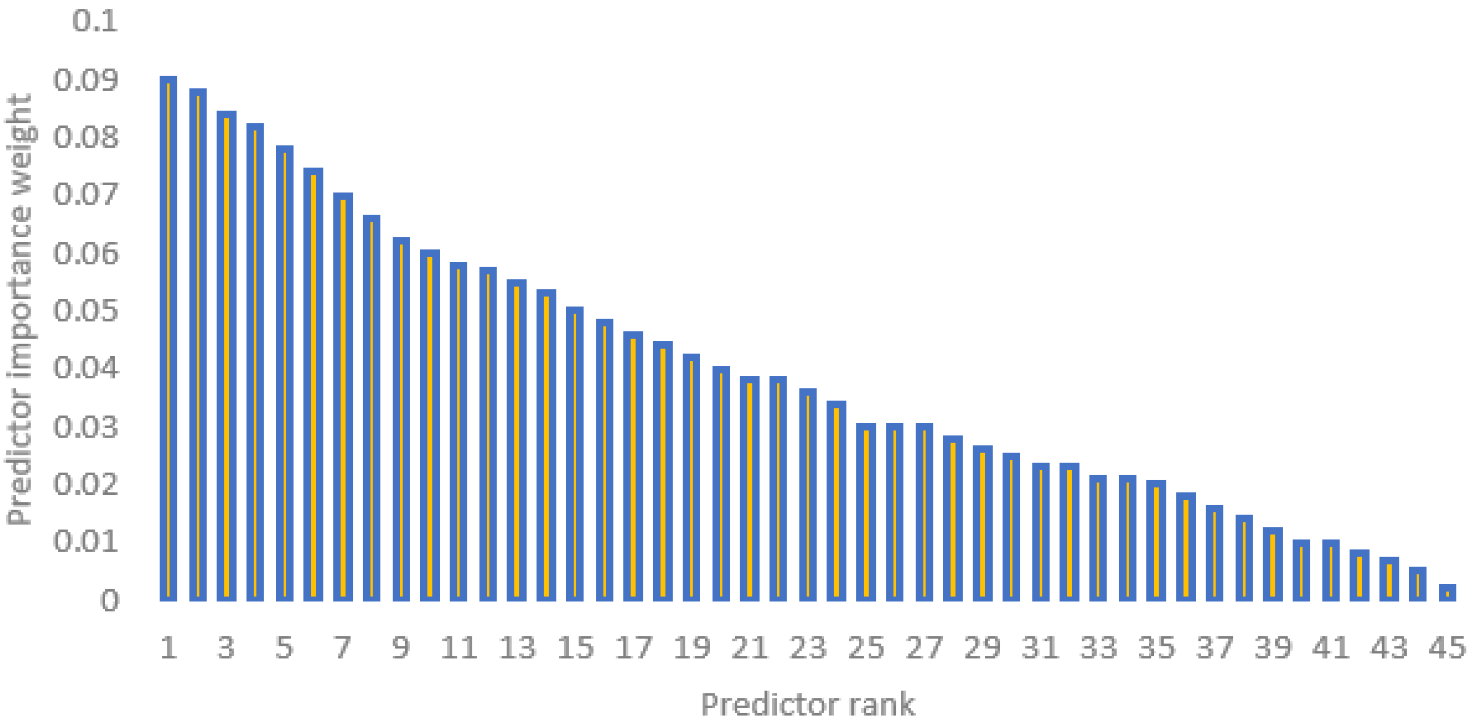
- Selecting relevant features through the ReliefF algorithm based on predictive importance weights;
- Fine-tuning DBN by elephant-herding optimization algorithm (EHO);
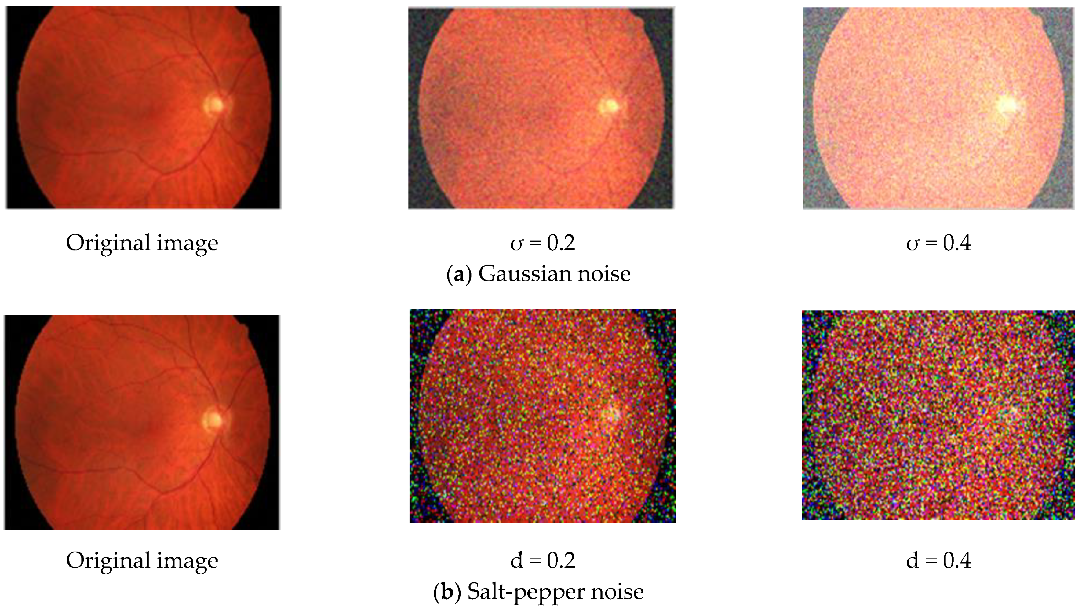
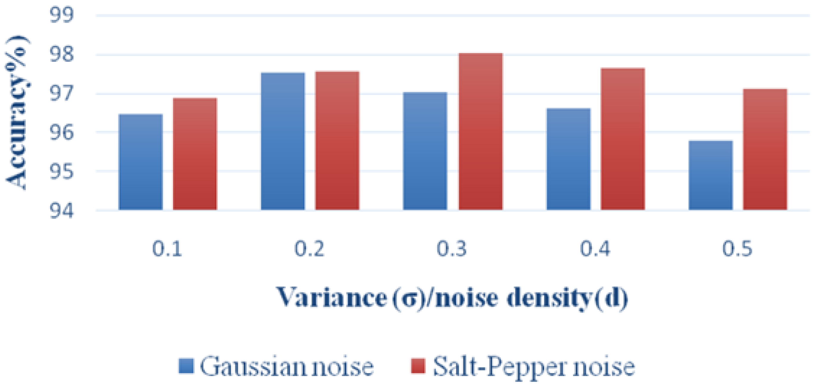
- Investigating the model’s robustness to noise such as Gaussian and salt-pepper;
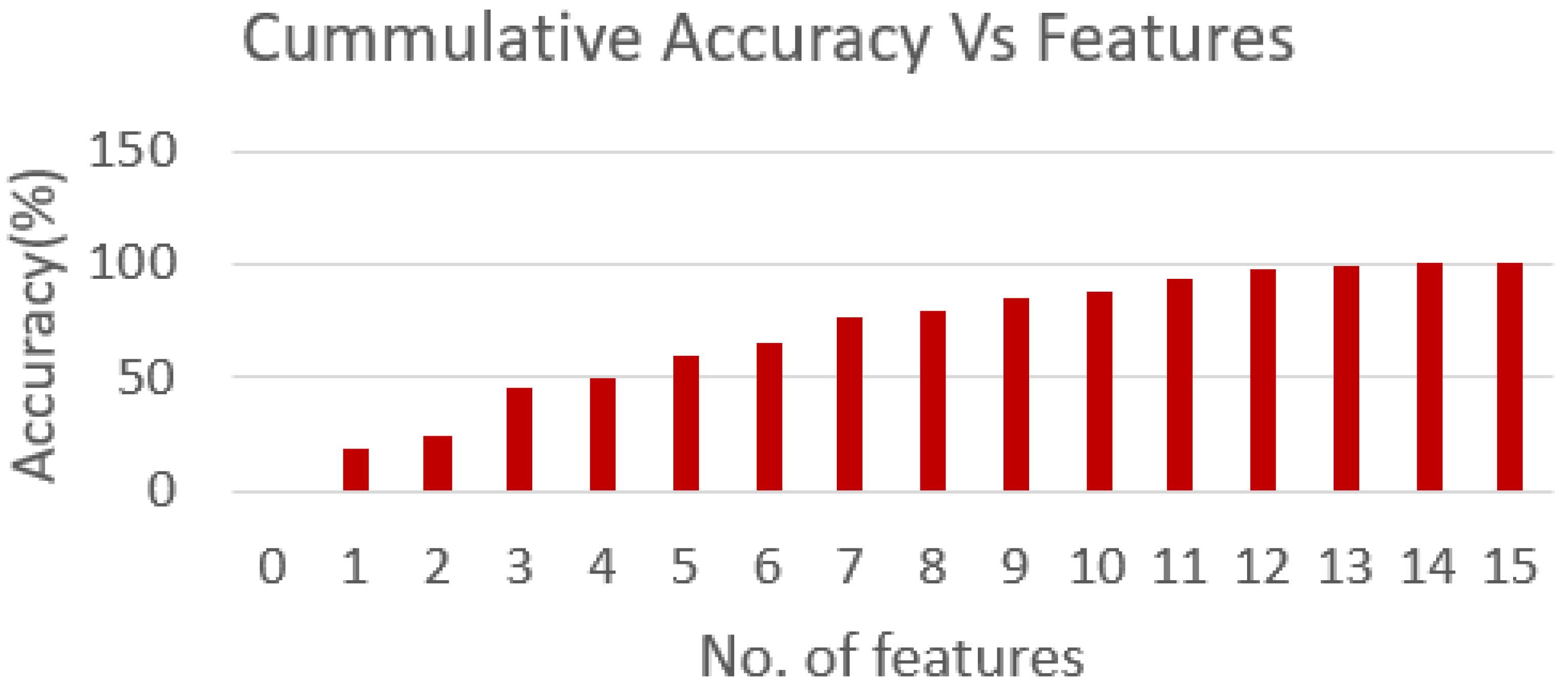
- Analyzing the isolated and combined feature set contribution in glaucoma identification.
2. Related Works
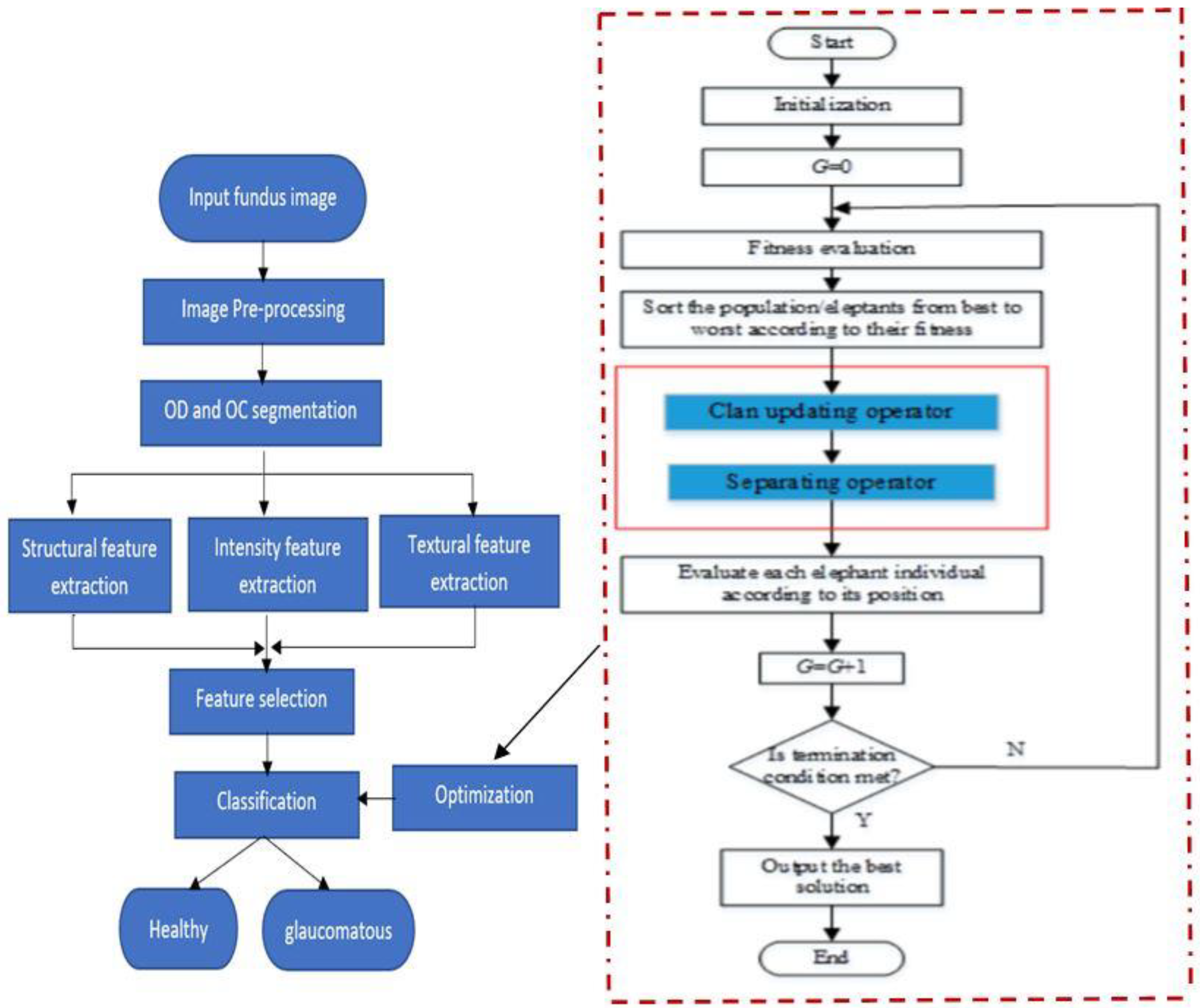
3. Proposed Method
3.1. Preprocessing
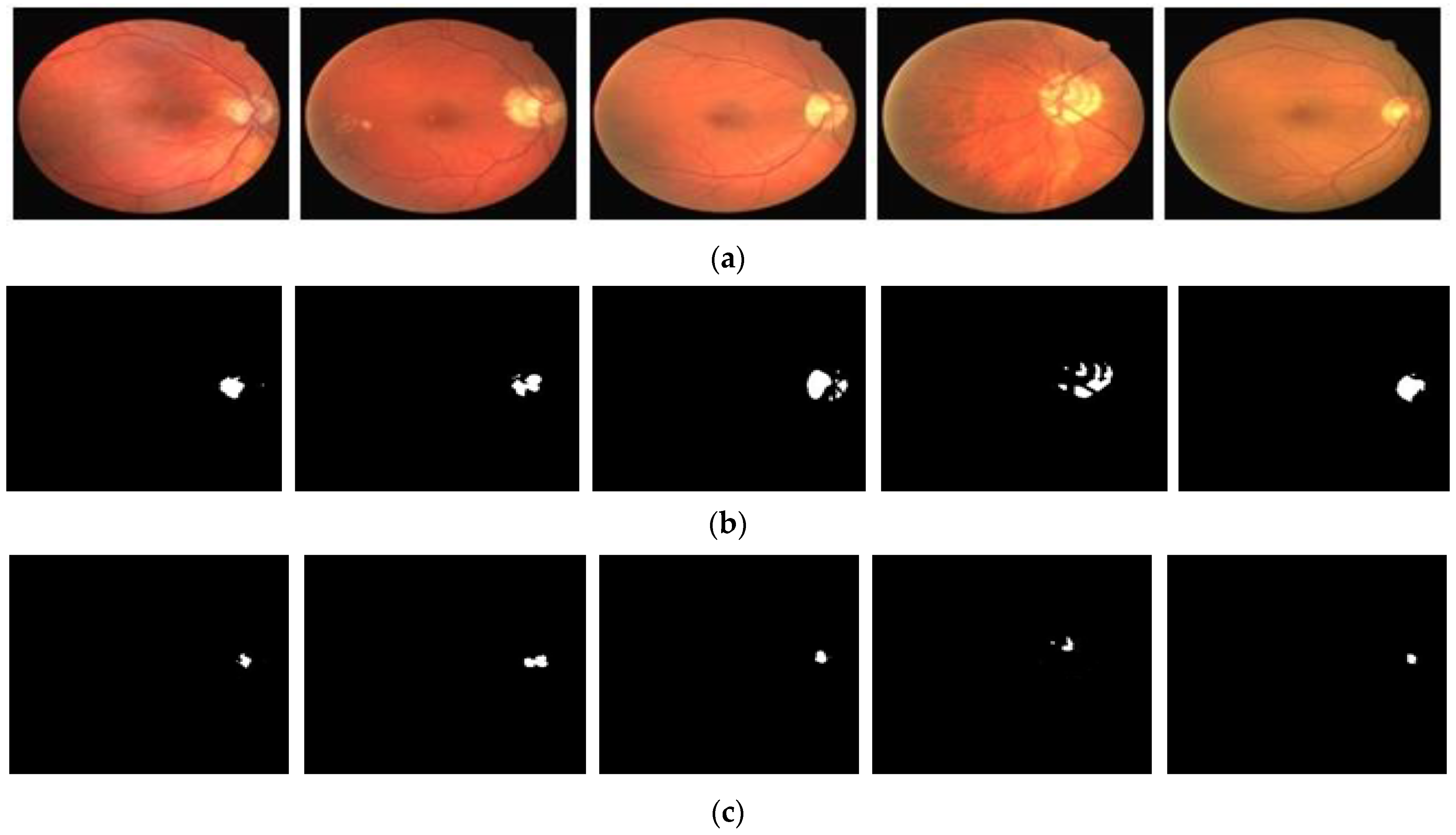
3.2. OD and OC Segmentation
3.3. Feature Extraction
3.4. Feature Selection
3.5. Classification
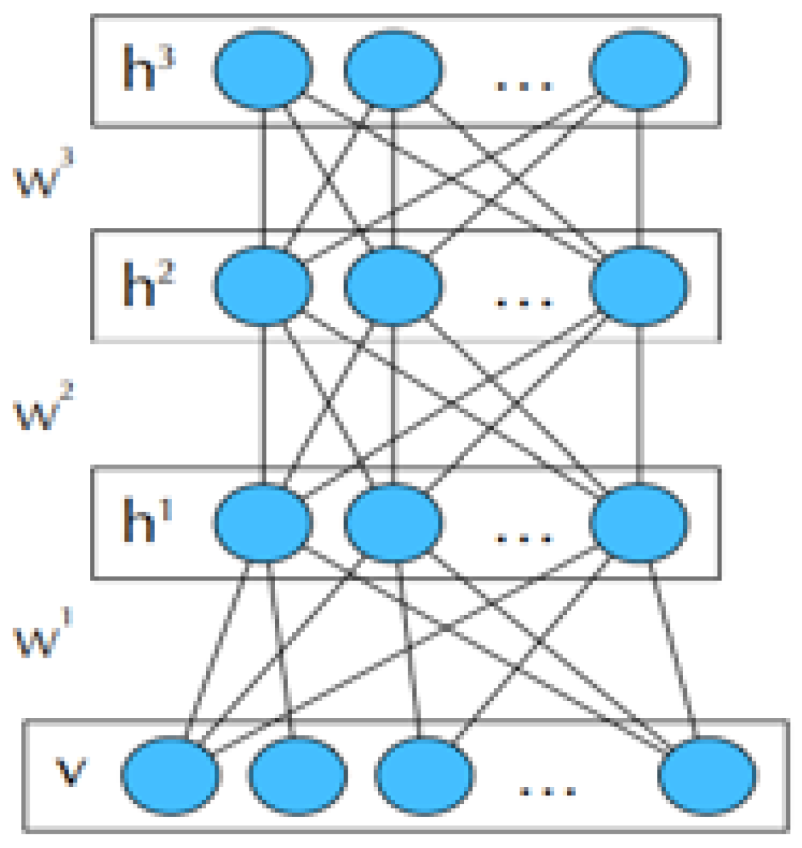
3.5.1. Deep Belief Networks (DBN)
3.5.2. Elephant Herd Optimization (EHO) Algorithm
- The elephant group is classified into clans, and each such clan comprises specific elephants.
- A specific number of male elephants (ME) depart their clan to live independently.
- Each clan has a leader termed the matriarch.
3.5.3. Fine Tuning of DBM
- Set the EHO parameters and initialize the population.
- Evaluate the individual fitness value (RMSE) of the DBN, as per the learning rate and the number of batch learning. Identify the optimal individual.
- Check if the termination condition is reached; if so, end the iteration and output the result; or else, go to the next step.
- Update each individual position. Reinitialize the individuals beyond the lower and upper limits.
- Start a new iteration by updating the optimal individual.
4. Results and Discussion
4.1. Dataset Preparation
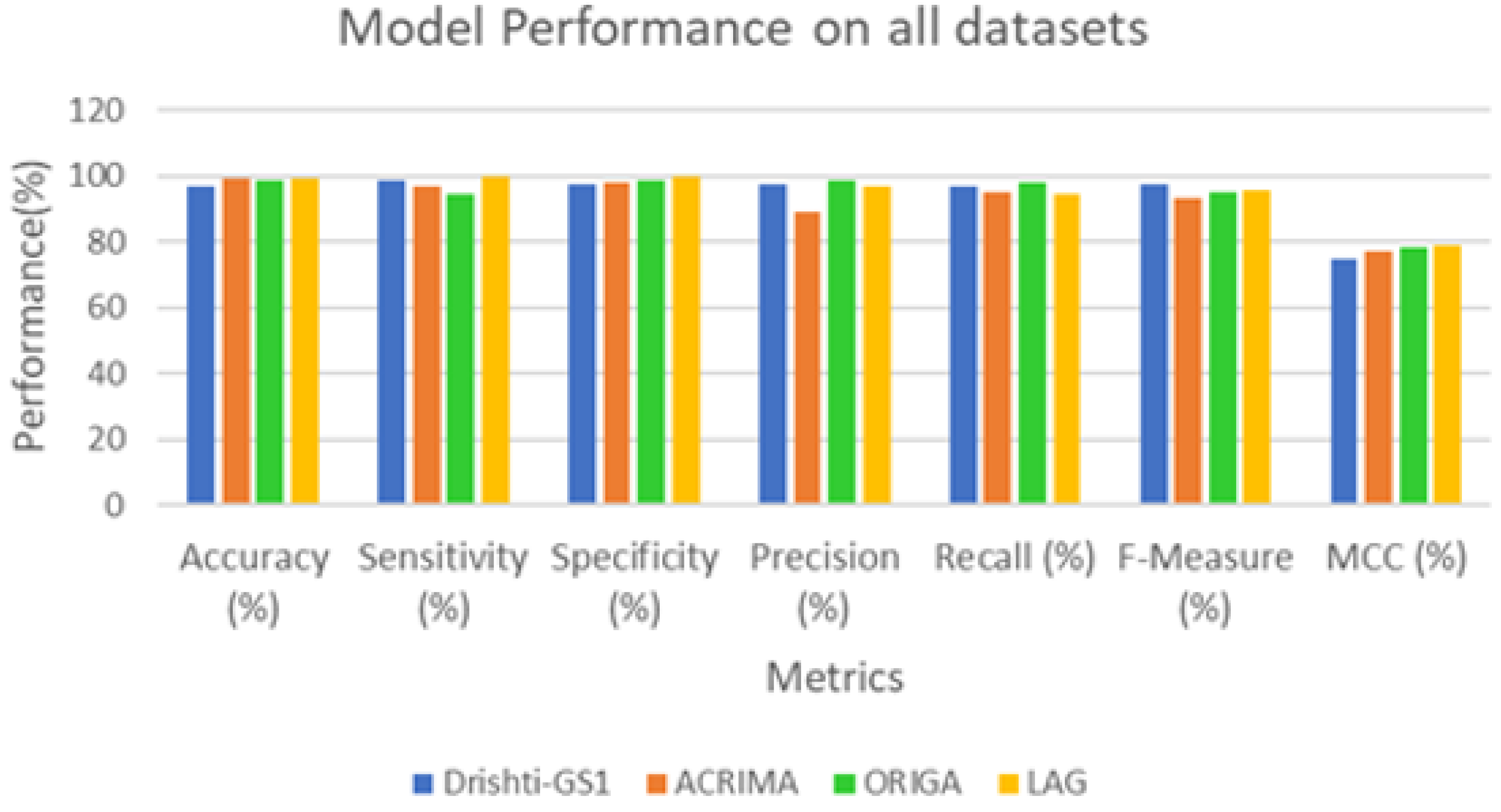
4.2. Performance Analysis
5. Conclusions
Author Contributions
Funding
Acknowledgments
Conflicts of Interest
References
- Quigley, H.A.; Broman, A.T. The number of people with glaucoma worldwide in 2010 and 2020. Br. J. Ophthalmol. 2006, 90, 262–267. [Google Scholar] [CrossRef] [PubMed] [Green Version]
- Dervisevic, E.; Pavlja, S.; Dervisevic, A.; Kasumovic, S.S. Challenges in early glaucoma detection. Med. Arch. 2017, 70, 203–207. [Google Scholar] [CrossRef] [PubMed] [Green Version]
- Kassebaum, N.J.; Bertozzi-Villa, A.; Coggeshall, M.S.; A Shackelford, K.; Steiner, C.; Heuton, K.R.; Gonzalez-Medina, D.; Barber, R.; Huynh, C.; Dicker, D.; et al. Global, regional, and national levels and causes of maternal mortality during 1990–2013: A systematic analysis for the Global Burden of Disease Study 2013. Lancet 2014, 384, 980–1004. [Google Scholar] [CrossRef] [Green Version]
- What Is Glaucoma? Available online: https://www.glaucoma.org/glaucoma/optic-nerve-cupping.php (accessed on 1 May 2021).
- McMonnies, C.W. Intraocular pressure and glaucoma: Is physical exercise beneficial or a risk? J. Optom. 2016, 9, 139–147. [Google Scholar] [CrossRef] [Green Version]
- Types of Glaucoma. Available online: http://www.glaucoma-association.com/about-glaucoma/types-of-glaucoma/chronic-glaucoma (accessed on 1 May 2021).
- Blindness. Available online: https://www.who.int/health-topics/blindness-and-vision-loss (accessed on 2 May 2021).
- Chandrika, S.; Nirmala, K. Analysis of CDR detection for glaucoma diagnosis. Int. J. Eng. Res. Appl. 2014, 2, 23–27. [Google Scholar]
- Al-Bander, B.; Al-Nuaimy, W.; Al-Taee, M.; Zheng, Y. Automated glaucoma diagnosis using deep learning approach. In Proceedings of the 14th International Multi-Conference on Systems, Signals & Devices (SSD), Marrakech, Morocco, 28–31 March 2017; pp. 207–210. [Google Scholar]
- Mardin, C.Y.; Horn, F.K.; Jonas, J.B.; Budde, W.M. Preperimetric glaucoma diagnosis by confocal scanning laser tomography of the optic disc. Br. J. Ophthalmol. 1999, 83, 299–304. [Google Scholar] [CrossRef] [Green Version]
- Adhi, M.; Duker, J.S. Optical coherence tomography—Current and future applications. Curr. Opin. Ophthalmol. 2013, 24, 213–221. [Google Scholar] [CrossRef] [Green Version]
- Septiarini, A.; Khairina, D.M.; Kridalaksana, A.H.; Hamdani, H. Automatic Glaucoma Detection Method Applying a Statistical Approach to Fundus Images. Healthc. Inform. Res. 2018, 24, 53–60. [Google Scholar] [CrossRef] [Green Version]
- Thorat, S.; Jadhav, S. Optic disc and cup segmentation for glaucoma screening based on super pixel classification. Int. J. Innov. Adv. Comput. Sci. 2015, 4, 167–172. [Google Scholar]
- Kavitha, K.; Malathi, M. Optic disc and optic cup segmentation for glaucoma classification. Int. J. Adv. Res. Comput. Sci. Technol. 2014, 2, 87–90. [Google Scholar] [CrossRef]
- Manju, K.; Sabeenian, R.S. Robust CDR calculation for glaucoma identification. Biomed. Res. 2018. [Google Scholar] [CrossRef] [Green Version]
- Mahalakshmi, V.; Karthikeyan, S. Clustering based optic disc and optic cup segmentation for glaucoma detection. Int. J. Innov. Res. Comput. Commun. Eng. 2014, 2, 3756–3761. [Google Scholar]
- Almazroa, A.; Burman, R.; Raahemifar, K.; Lakshminarayanan, V. Optic Disc and Optic Cup Segmentation Methodologies for Glaucoma Image Detection: A Survey. J. Ophthalmol. 2015, 2015, 180972. [Google Scholar] [CrossRef] [PubMed] [Green Version]
- Raja, C.; Gangatharan, N. A Hybrid Swarm Algorithm for optimizing glaucoma diagnosis. Comput. Biol. Med. 2015, 63, 196–207. [Google Scholar] [CrossRef] [PubMed]
- Issac, A.; Sarathi, M.P.; Dutta, M.K. An adaptive threshold based image processing technique for improved glaucoma detection and classification. Comput. Methods Programs Biomed. 2015, 122, 229–244. [Google Scholar] [CrossRef]
- Koh, J.E.W.; Ng, E.Y.K.; Bhandary, S.V.; Laude, A.; Acharya, U.R. Automated detection of retinal health using PHOG and SURF features extracted from fundus images. Appl. Intell. 2017, 48, 1379–1393. [Google Scholar] [CrossRef]
- Samanta, S.; Ahmed, S.K.; Salem, M.A.; Nath, S.S.; Dey, N.; Chowdhury, S.S. Haralick features based automated glaucoma classification using back propagation neural network. In Proceedings of the 3rd International Conference on Frontiers of Intelligent Computing: Theory and Applications (FICTA), Bhubaneswar, India, 14–15 November 2014; Springer: Cham, Switzerland, 2015; pp. 351–358. [Google Scholar]
- Cheng, J.; Liu, J.; Xu, Y.; Yin, F.; Wong, D.W.; Tan, N.M.; Tao, D.; Cheng, C.Y.; Aung, T.; Wong, T.Y. Superpixel classification based optic disc and optic cup segmentation for glaucoma screening. IEEE Trans. Med. Imaging 2013, 32, 1019–1032. [Google Scholar] [CrossRef]
- Singh, A.; Dutta, M.K.; ParthaSarathi, M.; Uher, V.; Burget, R. Image processing based automatic diagnosis of glaucoma using wavelet features of segmented optic disc from fundus image. Comput. Methods Programs Biomed. 2016, 124, 108–120. [Google Scholar] [CrossRef]
- Ajesh, F.; Ravi, R.; Rajakumar, G. Early diagnosis of glaucoma using multi-feature analysis and DBN based classification. J. Ambient. Intell. Humaniz. Comput. 2021, 12, 4027–4036. [Google Scholar] [CrossRef]
- Diaz, A.; Morales, S.; Naranjo, V.; Alcocer, P.; Lanzagorta, A. Glaucoma diagnosis by means of optic cup feature analysis in color fundus images. In Proceedings of the 24th European Signal Processing Conference (EUSIPCO), Budapest, Hungary, 29 August–2 September 2016; pp. 2055–2059. [Google Scholar]
- Gómez-Valverde, J.J.; Antón, A.; Fatti, G.; Liefers, B.; Herranz, A.; Santos, A.; Sánchez, C.I.; Ledesma-Carbayo, M.J. Automatic glaucoma classification using color fundus images based on convolutional neural networks and transfer learning. Biomed. Opt. Express 2019, 10, 892–913. [Google Scholar] [CrossRef] [Green Version]
- Diaz-Pinto, A.; Morales, S.; Naranjo, V.; Köhler, T.; Mossi, J.M.; Navea, A. CNNs for automatic glaucoma assessment using fundus images: An extensive validation. Biomed. Eng. Online 2019, 18, 29. [Google Scholar] [CrossRef] [PubMed] [Green Version]
- Raghavendra, U.; Fujita, H.; Bhandary, S.V.; Gudigar, A.; Tan, J.H.; Acharya, U.R. Deep convolution neural network for accurate diagnosis of glaucoma using digital fundus images. Inf. Sci. 2018, 441, 41–49. [Google Scholar] [CrossRef]
- Orlando, J.I.; Prokofyeva, E.; del Fresno, M.; Blaschko, M.B. Convolutional neural network transfer for automated glaucoma identification. In Proceedings of the 12th International Symposium on Medical Information Processing and Analysis, Tandil, Argentina, 5–7 December 2016. [Google Scholar]
- Chen, X.; Xu, Y.; Wong, D.W.; Wong, T.Y.; Liu, J. Glaucoma detection based on deep convolutional neural network. In Proceedings of the 2015 37th annual international conference of the IEEE engineering in medicine and biology society (EMBC), Milan, Italy, 25–29 August 2015; pp. 715–718. [Google Scholar]
- Staal, J.; Abràmoff, M.D.; Niemeijer, M.; Viergever, M.A.; Van Ginneken, B. Ridge-based vessel segmentation in color images of the retina. IEEE Trans. Med. Imaging 2004, 23, 501–509. [Google Scholar] [CrossRef]
- Hani, A.F.; Soomro, T.A.; Fayee, I.; Kamel, N.; Yahya, N. Identification of noise in the fundus images. In Proceedings of the 2013 IEEE International Conference on Control System, Computing and Engineering, Penang, Malaysia, 29 November–1 December 2013; pp. 191–196. [Google Scholar]
- Nagu, M.; Shanker, N. Image De-Noising by Using Median Filter and Weiner Filter. Int. J. Innov. Res. Comput. Commun. Eng. 2014, 2, 5641–5649. [Google Scholar]
- Aliskan, A.; Çevik, U. An Efficient Noisy Pixels Detection Model for C.T. Images using Extreme Learning Machines. Teh. Vjesn. —Tech. Gaz. 2018, 25, 679–686. [Google Scholar] [CrossRef]
- Raj, P.A.; George, A. FCM and Otsu’s Thresholding based Glaucoma Detection and its Analysis using Fundus Images. In Proceedings of the 2nd International Conference on Intelligent Computing, Instrumentation and Control Technologies (ICICICT), Kannur, India, 5–6 July 2019; pp. 753–757. [Google Scholar]
- Urbanowicz, R.J.; Meeker, M.; La Cava, W.; Olson, R.S.; Moore, J.H. Relief-based feature selection: Introduction and review. J. Biomed. Inform. 2018, 85, 189–203. [Google Scholar] [CrossRef]
- Rosa, G.; Papa, J.; Costa, K.; Passos, L.; Pereira, C.; Yang, X. Learning Parameters in Deep Belief Networks Through Firefly Algorithm. In Proceedings of the IAPR Workshop on Artificial Neural Networks in Pattern Recognition. In Artificial Neural Networks in Pattern Recognition. ANNPR 2016, Ulm, Germany, 28–30 September 2016; Lecture Notes in Computer Science. Springer: Cham, Switzerland, 2016; pp. 138–149. [Google Scholar]
- Hinton, G.E.; Osindero, S.; Teh, Y.-W. A Fast Learning Algorithm for Deep Belief Nets. Neural Comput. 2006, 18, 1527–1554. [Google Scholar] [CrossRef]
- Wang, G.-G.; Deb, S.; Coelho, L.d.S. Elephant Herding Optimization. In Proceedings of the 3rd International Symposium on Computational and Business Intelligence (ISCBI 2015), Bali, Indonesia, 7–8 December 2015; pp. 1–5. [Google Scholar]
- Li, J.; Lei, H.; Alavi, A.H.; Wang, G.-G. Elephant Herding Optimization: Variants, Hybrids, and Applications. Mathematics 2020, 8, 1415. [Google Scholar] [CrossRef]
- Nayak, M.; Das, S.; Bhanja, U.; Senapati, M.R. Elephant herding optimization technique based neural network for cancer prediction. Inform. Med. Unlocked 2020, 21, 100445. [Google Scholar] [CrossRef]
- Sivaswamy, J.; Krishnadas, S.R.; Joshi, G.D.; Jain, M.; Tabish, A.U.S. Drishti-GS: Retinal image dataset for optic nerve head (ONH) segmentation. In Proceedings of the IEEE 11th International Symposium on Biomedical Imaging (ISBI), Beijing, China, 29 April–2 May 2014; pp. 53–56. [Google Scholar]
- Khan, S.M.; Liu, X.; Nath, S.; Korot, E.; Faes, L.; Wagner, S.K.; Keane, P.A.; Sebire, N.J.; Burton, M.J.; Denniston, A.K. A global review of publicly available datasets for ophthalmological imaging: Barriers to access, usability, and generalisability. Lancet. Digit. Health 2021, 3, e51–e66. [Google Scholar] [CrossRef]
- Zhang, Z.; Yin, F.S.; Liu, J.; Wong, W.K.; Tan, N.M.; Lee, B.H.; Cheng, J.; Wong, T.Y. ORIGA(light): An on-line retinal fundus image database for glaucoma analysis and research. In Proceedings of the 2010 Annual International Conference of the IEEE Engineering in Medicine and Biology, Buenos Aires, Argentina, 31 August–4 September 2020; pp. 3065–3068. [Google Scholar]
- Li, L.; Xu, M.; Wang, X.; Jiang, L.; Liu, H. Attention Based Glaucoma Detection: A Large-Scale Database and CNN Model. In Proceedings of the IEEE/CVF Conference on Computer Vision and Pattern Recognition (CVPR), Long Beach, CA, USA, 15–20 June 2019; pp. 10563–10572. [Google Scholar]
- Karthikeyan, S.; Rengarajan, N. Performance Analysis of Gray Level Co-Occurrence Matrix Texture Features for Glaucoma Diagnosis. Am. J. Appl. Sci. 2014, 11, 248–257. [Google Scholar] [CrossRef]
- Mookiah, M.R.; Acharya, U.R.; Lim, C.M.; Petznick, A.; Suri, J.S. Data mining technique for automated diagnosis of glaucoma using higher order spectra and wavelet energy features. Knowl.-Based Syst. 2012, 33, 73–82. [Google Scholar] [CrossRef]
- Danandeh Mehr, A.; Rikhtehgar Ghiasi, A.; Yaseen, Z.M.; Sorman, A.U.; Abualigah, L. A novel intelligent deep learning predictive model for meteorological drought forecasting. J. Ambient. Intell. Humaniz. Comput. 2022, 24, 1–5. [Google Scholar] [CrossRef]
- Gharaibeh, M.; Almahmoud, M.; Ali, M.Z.; Al-Badarneh, A.; El-Heis, M.; Abualigah, L.; Altalhi, M.; Alaiad, A.; Gandomi, A.H. Early Diagnosis of Alzheimer’s Disease Using Cerebral Catheter Angiogram Neuroimaging: A Novel Model Based on Deep Learning Approaches. Big Data Cogn. Comput. 2021, 6, 2. [Google Scholar] [CrossRef]
- Gandomi, A.H.; Chen, F.; Abualigah, L. Machine Learning Technologies for Big Data Analytics. Electronics 2022, 11, 421. [Google Scholar] [CrossRef]
- Houssein, E.H.; Hassaballah, M.; Ibrahim, I.E.; AbdElminaam, D.S.; Wazery, Y.M. An automatic arrhythmia classification model based on improved Marine Predators Algorithm and Convolutions Neural Networks. Expert Syst. Appl. 2022, 187, 115936. [Google Scholar] [CrossRef]
- Houssein, E.H.; Abdelminaam, D.S.; Hassan, H.N.; Al-Sayed, M.M.; Nabil, E. A Hybrid Barnacles Mating Optimizer Algorithm with Support Vector Machines for Gene Selection of Microarray Cancer Classification. IEEE Access 2021, 9, 64895–64905. [Google Scholar] [CrossRef]
- Houssein, E.H.; Abdelminaam, D.S.; Ibrahim, I.E.; Hassaballah, M.; Wazery, Y.M. A Hybrid Heartbeats Classification Approach Based on Marine Predators Algorithm and Convolution Neural Networks. IEEE Access 2021, 9, 86194–86206. [Google Scholar] [CrossRef]
- Elminaam, D.A.; Ibrahim, S.A. Building a robust heart diseases diagnose intelligent model based on RST using lem2 and modlem2. In Proceedings of the 32nd IBIMA Conference, Seville, Spain, 15–16 November 2018; pp. 5733–5744. [Google Scholar]
- Abd Elminaam, D.S.; Elashmawi, W.H.; Ibraheem, S.A. HMFC: Hybrid MODLEM-Fuzzy Classifier for Liver Diseases Diagnose. Int. Arab. J. E Technol. 2019, 5, 100–109. [Google Scholar]
- Nadimi-Shahraki, M.H.; Taghian, S.; Mirjalili, S.; Ewees, A.A.; Abualigah, L.; Elaziz, M.A. MTV-MFO: Multi-Trial Vector-Based Moth-Flame Optimization Algorithm. Symmetry 2021, 13, 2388. [Google Scholar] [CrossRef]
- Nadimi-Shahraki, M.H.; Taghian, S.; Mirjalili, S.; Abualigah, L.; Elaziz, M.A.; Oliva, D. EWOA-OPF: Effective Whale Optimization Algorithm to Solve Optimal Power Flow Problem. Electronics 2021, 10, 2975. [Google Scholar] [CrossRef]
- Nadimi-Shahraki, M.H.; Fatahi, A.; Zamani, H.; Mirjalili, S.; Abualigah, L. An Improved Moth-Flame Optimization Algorithm with Adaptation Mechanism to Solve Numerical and Mechanical Engineering Problems. Entropy 2021, 23, 1637. [Google Scholar] [CrossRef] [PubMed]
- Elminaam, D.S.A.; Neggaz, N.; Ahmed, I.A.; Abouelyazed, A.E.S. Swarming Behavior of Harris Hawks Optimizer for Arabic Opinion Mining. Comput. Mater. Contin. 2021, 69, 4129–4149. [Google Scholar] [CrossRef]
- AbdElminaam, D.S.; Neggaz, N.; Gomaa, I.A.E.; Ismail, F.H.; Elsawy, A. AOM-MPA: Arabic Opinion Mining using Marine Predators Algorithm based Feature Selection. In Proceedings of the 2021 International Mobile, Intelligent, and Ubiquitous Computing Conference (MIUCC), Cairo, Egypt, 26–27 May 2021; pp. 395–402. [Google Scholar] [CrossRef]
- Shaban, H.; Houssein, E.H.; Pérez-Cisneros, M.; Oliva, D.; Hassan, A.Y.; Ismaeel, A.A.K.; AbdElminaam, D.S.; Deb, S.; Said, M. Identification of Parameters in Photovoltaic Models through a Runge Kutta Optimizer. Mathematics 2021, 9, 2313. [Google Scholar] [CrossRef]
- Deb, S.; Houssein, E.H.; Said, M.; Abdelminaam, D.S. Performance of Turbulent Flow of Water Optimization on Economic Load Dispatch Problem. IEEE Access 2021, 9, 77882–77893. [Google Scholar] [CrossRef]
- Abdul-Minaam, D.S.; Al-Mutairi, W.M.E.S.; Awad, M.A.; El-Ashmawi, W.H. An Adaptive Fitness-Dependent Optimizer for the One-Dimensional Bin Packing Problem. IEEE Access 2020, 8, 97959–97974. [Google Scholar] [CrossRef]
- El-Ashmawi, W.H.; Elminaam, D.S.A.; Nabil, A.M.; Eldesouky, E. A chaotic owl search algorithm based bilateral negotiation model. Ain Shams Eng. J. 2020, 11, 1163–1178. [Google Scholar] [CrossRef]
- Acharya, U.R.; Dua, S.; Du, X.; Chua, C.K. Automated diagnosis of glaucoma using texture and higher order spectra features. IEEE Trans. Inf. Technol. Biomed. 2011, 15, 449–455. [Google Scholar] [CrossRef]
- Acharya, U.R.; Ng, E.Y.; Eugene, L.W.; Noronha, K.P.; Min, L.C.; Nayak, K.P.; Bhandary, S.V. Decision support system for the glaucoma using Gabor transformation. Biomed. Signal Process. Control 2015, 15, 18–26. [Google Scholar] [CrossRef] [Green Version]
- Yadav, D.; Sarathi, M.P.; Dutta, M.K. Classification of glaucoma based on texture features using neural networks. In Proceedings of the 2014 Seventh International Conference on Contemporary Computing (IC3), Noida, India, 7–9 August 2014; pp. 109–112. [Google Scholar]
- Maheshwari, S.; Pachori, R.B.; Kanhangad, V.; Bhandary, S.V.; Acharya, U.R. Iterative variational mode decomposition based automated detection of glaucoma using fundus images. Comput. Biol. Med. 2017, 88, 142–149. [Google Scholar] [CrossRef]
- Bajwa, M.N.; Malik, M.I.; Siddiqui, S.A.; Dengel, A.; Shafait, F.; Neumeier, W.; Ahmed, S. Two-stage framework for optic disc localization and glaucoma classification in retinal fundus images using deep learning. BMC Med. Inform. Decis. Mak. 2019, 19, 1–6. [Google Scholar]
- Shehab, M.; Abualigah, L.; Shambour, Q.; Abu-Hashem, M.A.; Shambour, M.K.Y.; Alsalibi, A.I.; Gandomi, A.H. Machine learning in medical applications: A review of state-of-the-art methods. Comput. Biol. Med. 2022, 145, 105458. [Google Scholar] [CrossRef] [PubMed]
- Ezugwu, A.E.; Ikotun, A.M.; Oyelade, O.O.; Abualigah, L.; Agushaka, J.O.; Eke, C.I.; Akinyelu, A.A. A comprehensive survey of clustering algorithms: State-of-the-art machine learning applications, taxonomy, challenges, and future research prospects. Eng. Appl. Artif. Intell. 2022, 110, 104743. [Google Scholar] [CrossRef]
- Liu, Q.; Li, N.; Jia, H.; Qi, Q.; Abualigah, L. Modified Remora Optimization Algorithm for Global Optimization and Multilevel Thresholding Image Segmentation. Mathematics 2022, 10, 1014. [Google Scholar] [CrossRef]
- Gharaibeh, M.; Alzu’Bi, D.; Abdullah, M.; Hmeidi, I.; Al Nasar, M.R.; Abualigah, L.; Gandomi, A.H. Radiology Imaging Scans for Early Diagnosis of Kidney Tumors: A Review of Data Analytics-Based Machine Learning and Deep Learning Approaches. Big Data Cogn. Comput. 2022, 6, 29. [Google Scholar] [CrossRef]
- Zhang, W.; Li, X.; Ma, H.; Luo, Z.; Li, X. Universal Domain Adaptation in Fault Diagnostics with Hybrid Weighted Deep Adversarial Learning. IEEE Trans. Ind. Inform. 2021, 17, 7957–7967. [Google Scholar] [CrossRef]
- Zhang, W.; Li, X.; Li, X. Deep learning-based prognostic approach for lithium-ion batteries with adaptive time-series prediction and online validation. Measurement 2020, 164, 108052. [Google Scholar] [CrossRef]


| Structural Features | Cup to Disc Ratio (CDR), Neuro Retinal Rim (NRR), Cup Shape |
|---|---|
| Textural features | Wavelet-based features, gray level co-occurrence matrix (GLCM) features—energy, correlation, homogeneity, contrast, and entropy gray-level run length—low gray level run emphasis, gray level non-uniformity, segmentation-based fractal texture analysis (SFTA) |
| Intensity features | Brightness, color moments, super pixels, enhanced local binary pattern (ELBP), speeded-up robust feature (SURF), pyramid histogram of oriented gradients (PHOG), local energy-based shape histogram (LESH) |
| Database/Images | Normal | Glaucoma | Total | Type |
|---|---|---|---|---|
| DRISHIT-GSI [44] | 12 | 89 | 101 | Public |
| ACRIMA [29,45] | 309 | 396 | 705 | Public |
| OTIHS-lihjy [46] | 482 | 368 | 650 | Public |
| LAG [47] | 3432 | 2392 | 5824 | Private |
| Total | 4235 | 3045 | 7280 |
| Algorithm | Parameters |
|---|---|
| ABC | N = 30, MCN = 100, limit = 20 |
| HS | |
| FA | |
| CS | pa = 0.25 |
| PSO | Wmax = 0.9, Wmin = 0.2, C1 = 2, C2 = 2 |
| DE | F = 0.8, C = 0.5 |
| EHO |
| Algorithm | Layer-1 | Layer-2 | Layer-3 | |||
|---|---|---|---|---|---|---|
| CD | PCD | CD | PCD | CD | PCD | |
| ABC | 0.0891 | 0.8940 | 0.0881 | 0.0884 | 0.0880 | 0.0878 |
| HS | 0.1259 | 0.1345 | 0.1256 | 0.1169 | 0.1158 | 0.1156 |
| FA | 0.0864 | 0.0864 | 0.864 | 0.0860 | 0.0864 | 0.0862 |
| CS | 0.1146 | 0.1146 | 0.1176 | 0.1175 | 0.1164 | 0.1162 |
| PSO | 0.1086 | 0.1086 | 0.0988 | 0.0992 | 0.1045 | 0.1046 |
| DE | 0.1250 | 0.1254 | 0.1254 | 0.1254 | 0.1158 | 0.1156 |
| EHO | 0.0756 | 0.0756 | 0.0778 | 0.0778 | 0.0776 | 0.774 |
| Parameters | Expression |
|---|---|
| Sensitivity (%) | |
| Specificity (%) | 100 |
| Accuracy (%) | 100 |
| Precision (%) | 100 |
| Recall (%) | 100 |
| F-score (%) | 2 × 100 |
| Mathew’s correlation coefficient (MCC) (%) | 100 |
| Dataset | Acc (%) | Sens (%) | Spec (%) | Prec (%) | Recall (%) | F-Score (%) | MCC |
|---|---|---|---|---|---|---|---|
| Drishti-GS1 | 96.95 | 98.56 | 97.44 | 97.69 | 96.86 | 97.68 | 0.749 |
| ACRIMA | 99.34 | 97.1 | 98.2 | 88.92 | 95.3 | 93.5 | 0.772 |
| ORIGA | 98.51 | 94.73 | 98.7 | 98.55 | 97.92 | 95.32 | 0.784 |
| LAG | 99.31 | 99.89 | 100 | 96.73 | 94.56 | 95.64 | 0.789 |
| Features | Accuracy (%) | Sensitivity (%) | Specificity (%) |
|---|---|---|---|
| Structural (SF) | 94.87 | 95.32 | 93.52 |
| Intensity (IF) | 95.98 | 89.23 | 92.41 |
| Textural (TF) | 96.21 | 97.28 | 99.33 |
| SF + IF | 95.86 | 90.74 | 95.21 |
| SF + TF | 96.78 | 94.23 | 97.56 |
| IF + TF | 90.88 | 95.79 | 94.35 |
| Selected features | 99.31 | 99.89 | 100 |
| Dataset | Accuracy (%) |
|---|---|
| Drishti-GS1 | 97.1 |
| ACRIMA | 98.5 |
| ORIGA | 96.2 |
| LAG | 97.8 |
| Dataset | Classifier | Accuracy (%) | Sensitivity (%) | Specificity (%) |
|---|---|---|---|---|
| Drishti-GS | KNN | 95.34 | 90.47 | 93.08 |
| RF | 94.50 | 91.34 | 92.33 | |
| SVM | 95.86 | 96.87 | 96.87 | |
| DBN | 96.23 | 97.56 | 96.62 | |
| DBN–EHO | 96.95 | 98.56 | 97.44 | |
| ACRIMA | KNN | 95.66 | 90.86 | 93.78 |
| RF | 94.32 | 91.24 | 90.84 | |
| SVM | 97.06 | 96.64 | 96.12 | |
| DBN | 97.26 | 98.16 | 97.06 | |
| DBN–EHO | 99.34 | 97.1 | 98.2 | |
| ORIGA-Light | KNN | 94.22 | 96.86 | 97.08 |
| RF | 91.34 | 88.56 | 89.75 | |
| SVM | 94.88 | 95.56 | 96.69 | |
| DBN | 96.06 | 97.65 | 97.81 | |
| DBN–EHO | 98.51 | 94.73 | 98.7 | |
| LAG | KNN | 94.24 | 95.56 | 95.85 |
| RF | 92.78 | 90.89 | 91.48 | |
| SVM | 95.60 | 95.68 | 96.45 | |
| DBN | 97.54 | 95.67 | 97.43 | |
| DBN–EHO | 99.31 | 100 | 99.89 |
| Dataset | Classifier | Accuracy (%) | Sensitivity (%) | Specificity (%) |
|---|---|---|---|---|
| Drishti-GS | AlexNet | 93.84 | 91.57 | 92.88 |
| GoogLeNet | 95.46 | 90.34 | 93.36 | |
| VGG16 | 94.12 | 95.77 | 96.42 | |
| DBN-EHO | 96.95 | 98.56 | 97.44 |
| References | Features/Methods | Classifier Used | Images | Performance (%) |
|---|---|---|---|---|
| Karthikeyan and Rengarajan [65] | GLCM | BPN | Local dataset | Accuracy—95 |
| Issac, A. et al. [19] | CDR, NRR, blood vessel features | SVM and ANN | 67 | Accuracy—94.11 |
| Sensitivity—100 | ||||
| Mookiah et al. [66] | Discrete wavelet and HOS | SVM | 60 | Accuracy—95 |
| Sensitivity—93.3 | ||||
| Specificity—96.67 | ||||
| Gifta [24] | GLCM, HOG, SURF | Gray Wolf Optimized NN | N.A. | Accuracy—93.1 |
| Sensitivity—91.6 | ||||
| Specificity—94.1 | ||||
| Acharya, U.R. et al. [22] | 6 features from LM filter bank | KNN | NA | Accuracy—95.8 |
| Koh, J.E. et al. [20] | PHOG, SURF features | KNN | 910 | Accuracy—96.21 |
| Sensitivity—97.42 | ||||
| Samanta et al. [21] | Haralick features | BPN | 60 | Accuracy—96.26 |
| Sensitivity—90.43 | ||||
| Specificity—99.5 | ||||
| Acharya et al. [67] | Texture and HOF | RF | 60 | Accuracy—91 |
| Acharya et al. [68] | Gabor transformation and principal component analysis | SVM | 510 | Accuracy—93.10; sensitivity—89.75; specificity—96.20 |
| Yadav et al. [69] | Homogeneity, Contrast, energy, correlation, entropy | N.N. | 20 | Accuracy—72 |
| Maheshwari et al. [70] | Entropy and fractal | SVM | 488 | Accuracy—95.19 |
| Bajwa M. N et al. [71] | ROI, Scaling | 2-Stage CNN | ORIGA | AUC—0.87 |
| Raghavendra et al. [72] | - | 20 layer CNN | 1426 | Accuracy—98.13 |
| Chen et al. [73] | - | 16 layer CNN | SECS, ORIGA | AUC—0.881 |
| Proposed Work | Structural, intensity, and texture features | DBN and EHO | 7280 | Accuracy—99.34 |
| Sensitivity—100 | ||||
| Specificity—99.89 |
Publisher’s Note: MDPI stays neutral with regard to jurisdictional claims in published maps and institutional affiliations. |
© 2022 by the authors. Licensee MDPI, Basel, Switzerland. This article is an open access article distributed under the terms and conditions of the Creative Commons Attribution (CC BY) license (https://creativecommons.org/licenses/by/4.0/).
Share and Cite
Ali, M.A.S.; Balasubramanian, K.; Krishnamoorthy, G.D.; Muthusamy, S.; Pandiyan, S.; Panchal, H.; Mann, S.; Thangaraj, K.; El-Attar, N.E.; Abualigah, L.; et al. Classification of Glaucoma Based on Elephant-Herding Optimization Algorithm and Deep Belief Network. Electronics 2022, 11, 1763. https://doi.org/10.3390/electronics11111763
Ali MAS, Balasubramanian K, Krishnamoorthy GD, Muthusamy S, Pandiyan S, Panchal H, Mann S, Thangaraj K, El-Attar NE, Abualigah L, et al. Classification of Glaucoma Based on Elephant-Herding Optimization Algorithm and Deep Belief Network. Electronics. 2022; 11(11):1763. https://doi.org/10.3390/electronics11111763
Chicago/Turabian StyleAli, Mona A. S., Kishore Balasubramanian, Gayathri Devi Krishnamoorthy, Suresh Muthusamy, Santhiya Pandiyan, Hitesh Panchal, Suman Mann, Kokilavani Thangaraj, Noha E. El-Attar, Laith Abualigah, and et al. 2022. "Classification of Glaucoma Based on Elephant-Herding Optimization Algorithm and Deep Belief Network" Electronics 11, no. 11: 1763. https://doi.org/10.3390/electronics11111763