An Optimal Procedure for the Design of Discrete Constrained Lens Antennas with Minimized Optical Aberrations. Part I: Two-Dimensional Architectures

Abstract

Despite to the significant literature available on the design and applications of two-dimensional constrained lens antennas, and in particular on the Rotman–Turner lens, a rigorous study focused on the minimization of optical aberrations does not seem to be available. A general procedure for the design of two-dimensional bootlace lens antennas with a flat front profile is proposed in this paper. For the 3-foci lens, the best performance is achievable when, in addition to the three nominal focal points, two additional symmetric quasi foci are present. For the 4-foci lens the best performance is obtained when the presence of one additional quasi focus on the lens axis is guaranteed. Both the 3- and 4-foci lenses, when optimized, converge to the same configuration which exhibits aberrations following a Chebyshev-like behavior and guarantees quasi 5 foci. The optimized lens architecture is such that, for every scanning angle, the aberrations in the two extreme points are the most significant and exhibit opposite values. Any variation from this optimal condition implies increased aberrations. Although a 5-foci lens with flat front profile cannot be derived, one quasi-5-foci lens is derived asymptotically starting from two completely different lens architectures. A maximization of the number of foci combined with a rigorous derivation of the focal curve turned to be the key driver to identify an optimal two-dimensional bootlace lens. The quasi 5-foci lens presented can be considered the optimum Rotman–Turner lens in terms of optical aberrations allowing to reduce the optical aberrations by about one order of magnitude as compared to the best results available in the literature.

1. Introduction

Discrete lens antennas are also known as bootlace lenses, constrained lenses, or discretized array lenses [1]. Two-dimensional (parallel plate configuration) bootlace lenses have been investigated intensively in the literature, starting from some seminal contributions [2,3,4]. The success of the two-dimensional lenses is justified by their design simplicity, their modularity and scalability and other properties they share with three-dimensional discrete lenses. Two-dimensional constrained lenses can be designed to have more than one focal point. The wide-angle scanning capabilities of these lenses in two dimensions is well established, being larger when increasing the number of focal points [1,2,3,4]. In particular, the Rotman–Turner lens [4], characterized by one central focus, two symmetrical lateral foci and a flat front lens profile, has found several applications including satellite ones. The main benefits associated with this type of discrete lens BFN are associated with the simple implementation in Printed Circuit Board Technology (PCB), the excellent scanning capabilities, the fact that the front aperture is completely flat making the interfaces with other devices and/or antennas particularly easy. The quasi free-space beamforming, and the true-time delay behavior represent also two unique and fundamental advantages that justify the increasing utilization of this type of beamforming network in several applications.

Although Rotman lenses have been used for a long time and several publications on their design are available (see, for instance, [5,6,7,8]), to the best of our knowledge an optimal and general procedure to dimension this class of lenses has not been derived yet. In [5,6,7,8] useful guidelines to preliminarily define this type of antennas are proposed. A rigorous and generalized procedure to design two-dimensional constrained discrete lens antennas with a flat front profile is proposed here. In particular, two-dimensional discrete lens BFN and antennas characterized by 1, 2, 3 and 4 focal points are considered. The R-2R lens is also considered as a reference [9,10]; it exhibits an infinite number of focal points, but its front profile is curved. One may wonder why the 3-foci bootlace lens [2,3,4,5,6,7,8], mostly known as Rotman or Rotman–Turner lens, has gained a huge popularity while the R-2R, with an infinite number of foci, is hardly used. In some papers it is mentioned that the R-2R has a limited field of view. However, the R-2R exhibits excellent scanning performance up to ~±60°, which represents a really large field of view for several applications, and is larger as compared to the field of view typically reachable with a 3-foci lens. Clapp devised a means to use four or six R-2R lenses to feed a full 360° aperture, but the hardware design is further complicated by several hybrids for each beam [11]. In our opinion, it is the curved profile of the front lens in the R-2R configuration that limits its applicability and its compatibility and integration with other components (like a second block of two-dimensional lenses orthogonal to the first [12,13]). In addition, the R-2R lens cannot exhibit a magnification factor different from 1.

The paper contains several new results: (a) the procedure to minimize the lens optical aberrations, (b) the relations between the constitutive parameters, (c) an accurate estimation of the optical aberrations achievable with these lenses as a function of the constitutive parameters (including the effects of the ratio between the focal distance over the diameter, and a possible arbitrary zooming or magnification factor). The analytical and heuristic relations reported permit the antenna designer to identify quickly promising configurations and the performance achievable in terms of accommodation, volume, optical aberrations.

In the paper the dimensions of the radiating elements constituting the focal feeding array, the back array and the front array are never indicated. This point does not represent a limitation at all. In fact, all the results presented (i.e., the profiles, the phase shifters, the aberrations and all the equations) remain valid for any possible dimension for the radiating elements that the designer may choose.

The paper is organized as follows. In Section 2, the constitutive parameters of two-dimensional bootlace lenses are introduced. In Section 3, different lens architectures are defined. In Section 4 and Section 5, an optimal procedure to optimize 3-foci and 4-foci lenses in such a way they exhibit minimized optical aberrations is proposed. Numerical results are reported in Section 6, while Section 7 summarizes the properties derived in the paper.

2. Variables Definition

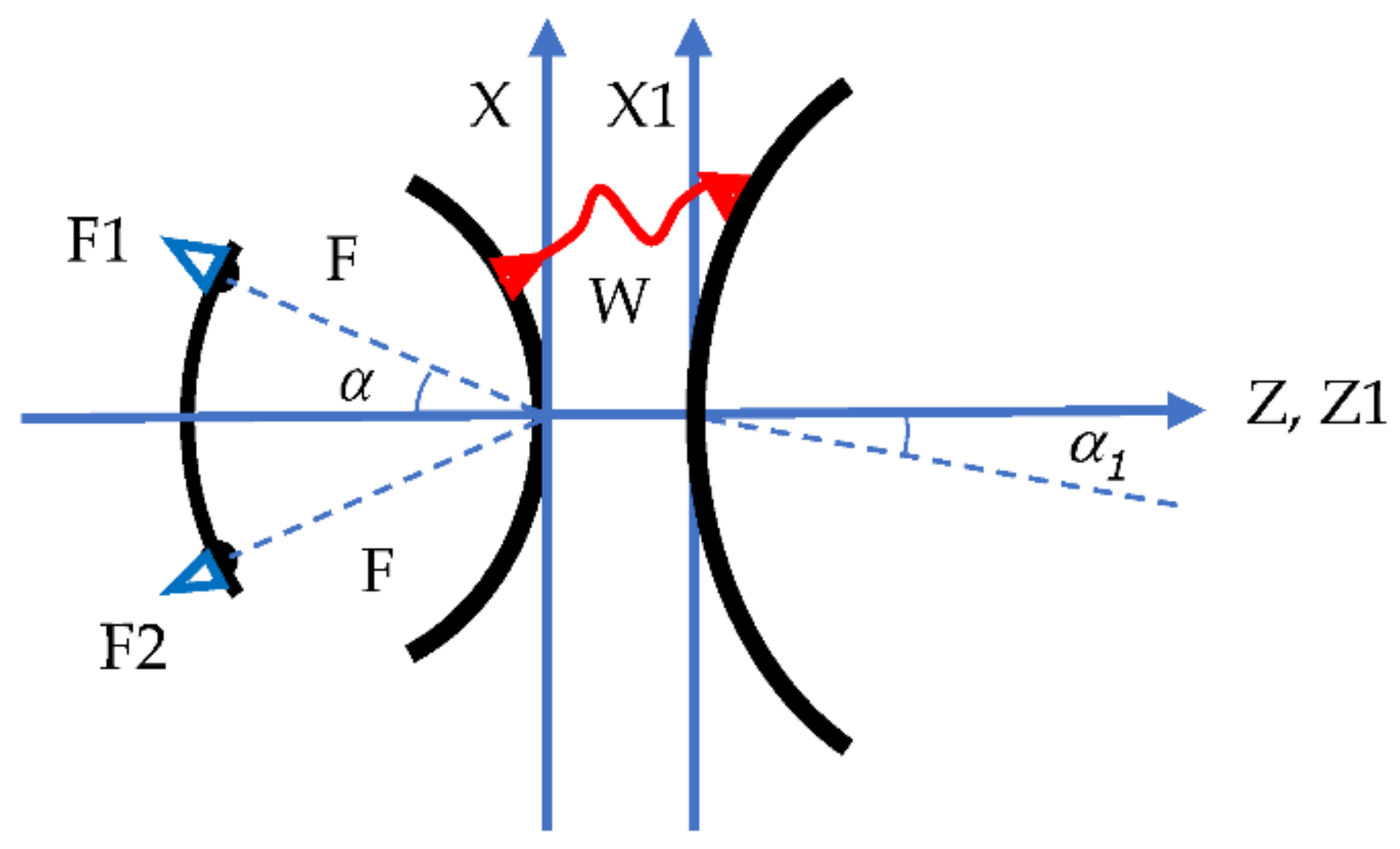
In the paper the two-dimensional bootlace lenses are defined adopting the Cartesian coordinate system shown in Figure 1.

The front lens profile is defined with the coordinates (X1, Z1), the back lens profile with the coordinates (X, Z); the transmission lines lengths with the variable W, the foci with the letters F1, F2; the focal distances with the letter F, G or H. The angles defining the positions of the foci in the X–Z plane with the letter $\mathsf{\alpha }$ or $\mathsf{\delta }.$ The homologous angles defining the pointing direction of the lens are identified with $\mathsf{\alpha }1$ and $\mathsf{\delta }1$. Bootlace lenses, like other optical systems based on reflectors [14,15], permit to generate plane waves pointing in directions characterized by an angle α1 which can be larger or smaller as compared to the angle α defining the position of the corresponding focal point. In optics, this property is indicated as Magnification or Zooming or Imaging. In 1967, Raytheon recognized that this property for 2D bootlace lenses constitutes a useful additional degree of freedom. When the zooming is not included α1 = α, δ1 = δ. In the paper, the magnification or zooming factor is indicated with letter M and can be defined:

$$\begin{gathered} \sin \left(\mathsf{\alpha }1\right)=\sin \left(\mathsf{\alpha }\right)\mathrm{M}, cos\left(\mathsf{\alpha }1\right)={\left(1-{\left(\sin \left(\mathsf{\alpha }\right)\mathrm{M}\right)}^2\right)}^{\frac{1}{2}} \\ \sin \left(\mathsf{\delta }1\right)=\sin \left(\mathsf{\delta }\right)\mathrm{M}, cos\left(\mathsf{\delta }1\right)={\left(1-{\left(\sin \left(\mathsf{\delta }\right)\mathrm{M}\right)}^2\right)}^{\frac{1}{2}} \end{gathered}$$

When M < 1, the pointing angles of the beams emerging from the lens are smaller as compared to the angles defining the position of the homologous feeding point. Vice versa, when M > 1, the pointing angles of the beams emerging from the lens are larger than the angles defining the homologous feeding point. As an off-axis beam can emerge from the array at an angle greater than, or lower than, the angle from the on-axis focus to the driven beam port, the zooming parameter M can be named also the expansion, or compression, factor. In order to achieve a magnification factor M, the back lens diameter must be approximately equal to the diameter of the front lens multiplied by M. In [1], possible antenna architectures exploiting this magnification property are identified.

To define a two-dimensional discrete lens, the following five variables are needed: X, Z, W, X1 and Z1. Choosing one variable as an independent variable (usually the X1 is selected), 5 − 1 = 4 free variables remain. They represent the degrees of freedom in the design and the maximum number of geometrical optics (GO) perfect foci. In facts, two-dimensional discrete lenses may exhibit up to four foci. The R-2R bootlace lens represents an exception because is a two-dimensional discrete lens with an infinite number of foci. In the paper the wavelength is denoted, as usually, with the symbol λ. The axial focal distance is denoted by G, the off axis focal distances associated to perfect foci with F, the focal distance associated to an arbitrary feed not coinciding with a perfect focus with the letter H.

3. Two-Dimensional Lens Architectures

In this section, two-dimensional discrete lens antennas are defined adopting simple analytical formulations. Although these configurations are not new, the analytical expressions in explicit form reported here are essential for the following discussion. Usually, these two-dimensional discrete lenses are realized in parallel-plate waveguide adopting a dielectric material in the lens cavity in order to miniaturize the cavity. In this paper, the effects of the dielectric constant are not included in the formulation and the discussion. However, this hypothesis does not represent a limitation because the dielectric constant simply implies a scaling factor on the dimensions of the back lens and focal arc.

• Configuration with 1 focal point:

  $$\begin{array}{l}\mathrm{Z}1=0,\\ \mathrm{X}=\mathrm{X}1 \mathrm{M},\\ \mathrm{Z}=-\mathrm{F}+{\left({\mathrm{F}}^2-{\mathrm{X}}^2\right)}^{\frac{1}{2}},\\ \mathrm{W}=0;\end{array}$$
• Configuration with 2 focal points:

  $$\begin{array}{l}\mathrm{Z}1=0\\ \mathrm{X}=\mathrm{X}1 \mathrm{M}\\ Z=-Fca+{\left({\left(Fca\right)}^2-{\left(Xca\right)}^2\right)}^{\frac{1}{2}}\\ \mathrm{W}=0;\end{array}$$
• Configuration with 3 focal points
  (better known as Rotman-Turner lens). The formulation of Hansen [5] and Simon [6], particularly compact, is proposed here.

  $$\begin{array}{l}\beta =\mathrm{F}/\mathrm{G},\\ \mathrm{M}=zoom=\mathrm{sa}1/\mathrm{sa},\\ \zeta =\mathrm{X}1 \mathrm{M}/\mathrm{G},\\ a=1-\frac{{\left(1-\beta \right)}^2}{{\left(1-\beta ca\right)}^2}-{\zeta }^2/{\beta }^2,\\ b=-2+2\frac{{\zeta }^2}{\beta }+2\frac{\left(1-\beta \right)}{\left(1-\beta \mathrm{ca}\right)}-{\zeta }^2{\mathrm{sa}}^2\left(1-\beta \right)/{\left(1-\beta \mathrm{ca}\right)}^2,\\ c=-{\zeta }^2+{\zeta }^2{\mathrm{sa}}^2/\left(1-\beta ca\right)-{\zeta }^4{\mathrm{sa}}^4/\left(4{\left(1-\beta \mathrm{ca}\right)}^2\right),\\ \mathrm{W}=\mathrm{G}\left(-b-\mathrm{sqrt}\left(b^2-4ac\right)\right)/\left(2a\right),\\ \mathrm{Z}=\mathrm{G}\left(-\left(0.5 {\zeta }^2{\mathrm{sa}}^2+\left(1-\beta \right)\mathrm{W}/\mathrm{G}\right)/\left(1-\beta \mathrm{ca}\right) \right),\\ \mathrm{X}=\mathrm{G} \zeta \left(1-\mathrm{W}/\mathrm{G}/\beta \right),\\ \mathrm{Z}1=0;\end{array}$$
• Configuration with 4 focal points:

  $$\begin{array}{l}\mathrm{X} = \mathrm{X}1 \mathrm{M}/\mathrm{F}{\left(\frac{4{\mathrm{F}}^4-4F^2\mathrm{X}{1}^2{\mathrm{M}}^2\left(1+\mathrm{ca} \mathrm{cd}\right)+\mathrm{X}{1}^4{\mathrm{M}}^4{\left(\mathrm{ca}+\mathrm{cd}\right)}^2}{{\mathrm{F}}^2-\mathrm{X}{1}^2{\mathrm{M}}^2}\right)}^{\frac{1}{2}}/2,\\ Z=-\mathrm{X}{1}^2{\mathrm{M}}^2\left(\mathrm{ca}+\mathrm{cd}\right)/\left(2\mathrm{F}\right)\\ \mathrm{W} = \mathrm{F} -{\left(\frac{4{\mathrm{F}}^4-4{\mathrm{F}}^2\mathrm{X}{1}^2{\mathrm{M}}^2\left(1+\mathrm{ca} \mathrm{cd}\right)+\mathrm{X}{1}^4{\mathrm{M}}^4{\left(\mathrm{ca}+\mathrm{cd}\right)}^2}{{\mathrm{F}}^2-\mathrm{X}{1}^2{\mathrm{M}}^2}\right)}^{\frac{1}{2}}/2,\\ \mathrm{Z}1=0;\end{array}$$

  where sa = sin($\mathsf{\alpha }$), sd = sin(δ), ca = cos($\alpha$), cd = cos (δ), sa1 = sin($\mathsf{\alpha }1$)

The 4-foci lens is characterized by the angles +α, −α, +δ, −δ, so there are two couples of symmetrical foci. The 4 associated focal distances have to be identical in order to have a configuration characterized by real quantities. It is important to note that the equation defining Z represents a parabolic function with a curvature depending on the focal distance, magnification factor and opening angles α and δ. However, the back profile is exactly parabolic as compared to the independent variable X1 but not as compared to the X variable. In practice, since the relation between X and X1 is quasi-linear, the back profile shape can be considered quasi-parabolic. It is interesting to note also that X1 is used as independent variable. When trying to use X as independent variable in order to derive (X1, Z, W) instead of (X, Z, W), the solutions can be obtained as a function of the roots of an equation of 6th degree.

E.

Configuration with ∞ focal points: R-2R lens [9,10]:

$$\begin{array}{l}\mathrm{X}=\mathrm{X}1\frac{{\left({\mathrm{G}}^2-\mathrm{X}{1}^2\right)}^{\frac{1}{2}}}{\mathrm{G}},\\ \mathrm{W}=0,\\ \mathrm{Z}=-\mathrm{G}/2+{\left({\left(\frac{\mathrm{G}}{2}\right)}^2-{\mathrm{X}}^2\right)}^{\frac{1}{2}},\\ \mathrm{Z}1=-\mathrm{G}+{\left({\mathrm{G}}^2-\mathrm{X}{1}^2\right)}^{\frac{1}{2}};\end{array}$$

Note: in case the X is selected as independent variable it is possible to find analytical expressions in explicit form:

$$\begin{array}{l}\mathrm{W} =0,\\ \mathrm{Z} =-\mathrm{G}/2+sqrt{\left({\left(\frac{G}{2}\right)}^2-{\mathrm{X}}^2\right)}^{\frac{1}{2}},\\ \mathrm{Z}1=-\mathrm{G} +sqrt{\left({\mathrm{G}}^2-\mathrm{X}{1}^2\right)}^{\frac{1}{2}},\\ \mathrm{X}1={\left(\frac{\mathrm{G}\left(\mathrm{G} -{\left({\mathrm{G}}^2-4{\mathrm{X}}^2\right)}^{\frac{1}{2}}\right)}{2}\right)}^{\frac{1}{2}}.\end{array}$$

This lens is well known to have infinite focal points located in the same circle constituting the back lens profile. It is able to scan up to ~±60°.

4. Optimization of 3-Foci Lenses

The analytical expressions presented in Section 3 permit defining: (a) the front lens profile (i.e., Z1 as a function of X1); (b) the back lens profile (i.e., Z as a function of X or X1); (c) the function W representing the constrained phase shift between the back and front lens (i.e., W as a function of X or X1); (d) the relation between the front and the back transversal coordinates (i.e., X as a function of X1, or X1 as a function of X); (e) the magnification or zooming factor (i.e., the relation between the pointing angle of the local beam versus the opening angle of the corresponding feed as compared to the central longitudinal axis of the lens). However, these analytical expressions permit to define completely only the R-2R lens because in this lens the focal arc is defined as well and coincides with the circle representing the back lens profile. For the other configurations, the lens architecture is not completely defined yet. Let us start by discussing about the 3-foci lens with flat front aperture. In this lens, the optimal relation between the two focal distances G and F (associated, respectively, to the central on axis focus and the two lateral foci in symmetrical positions) is not known. Therefore, the first challenge is, for the 3-foci lens, the identification of the optimal F/G ratio.

The second challenge consists in identifying the focal arc shape based on different possible criteria. First of all, the focal arc should pass through the focal points, or close by, in order to guarantee minimized aberrations at least in the vicinity of the focal points. Then, a focal arc profile should be defined because the number of beams usually required is much higher as compared to the number of focal points. In the literature, circular, or elliptical, or parabolic focal arc profiles have been proposed. This type of choice implies advantages in terms of manufacturability. In this paper, it will be shown that a different type of focal arc profile should be adopted if the priority in the design is the minimization of the maximum aberrations versus the scanning angles for an assigned focal distance (so for an assigned volumetric envelope for the lens architecture).

The opening angle α of the lens associated with the two symmetrical focal points is considered assigned. One of the two focal distances—G, associated to the central focal point (located on the lens axis), or F, associated to the lateral focal points, is considered assigned. Let us start identifying the second focal distance by adopting a procedure more rigorous as compared to the ones previously proposed in the literature.

Step 1:

Estimation of the second focal distance.

As a first step, instead of fixing as target the minimization of the maximum aberration in the entire field of view comprised between the extreme angles (−α and +α), it is more effective to derive the second focal distance in such a way to minimize the minimum optical aberration inside the field of view. In practice, as a rule of thumb, the second focal distance is derived trying to minimize the aberration in an intermediate angle γ:

sin(γ) ~ (α in radians)/π = (α in degrees)/180

(1)

In this intermediate angle γ, the following expression represents a good approximation for the relation between the two focal distances G and F:

$$\mathrm{F}=\mathrm{G}\left(\mathsf{\alpha }-\frac{{\mathsf{\alpha }}^3}{6}-\frac{{\mathsf{\alpha }}^5}{12}\right)/\sin \left(\mathsf{\alpha }\right)$$

(2)

Equations (1) and (2) are heuristic and have been derived empirically after several optimizations. It has also been validated for different values of the α angle, defining the positions of the two lateral foci. This new Equation (2) represents a more general and accurate relation as compared to the rule of thumb relations presented in the literature in the last 50 years (that have been mainly validated for a specific angle, typically α = 30°).

Step 2:

Estimation of the focal arc.

For every pointing direction, associated with a generic angle δ, the local focal distance is derived by enforcing that the aberrations associated with the two extreme points of the lens, i.e., the ones characterized by a minimum and maximum value for the transversal coordinate X1 (and X), are equal in term of absolute value but opposite in terms of sign. This assumption, combined with the Equations (1) and (2), is instrumental in order to obtain a quasi-Chebyshev behavior for the optical aberrations and the possibility to obtain two additional quasi-foci in addition to the three assigned ones. This choice guarantees a locally optimum solution as small variations from the optimized values imply an increase of the aberrations. The focal distance associated to a generic angle $\mathsf{\delta }$ can be expressed by:

$$\mathrm{Hz}=-\mathrm{H}{\left(1-{\mathrm{u}}^2\right)}^{\frac{1}{2}}; \mathrm{Hx}=\mathrm{H} \mathrm{u}; \mathrm{u}=\sin \left(\delta \right);$$

The aberrations in the positive and negative extremal points of the lens have to satisfy, respectively, the following two equations:

$$\begin{array}{l}\mathrm{Aberration}\left(\mathrm{in}+\mathrm{X}\right)={\left({\left(\mathrm{Hx}-\mathrm{X}\right)}^2+{\left(\mathrm{Hz}-\mathrm{Z}\right)}^2\right)}^{\frac{1}{2}}+\mathrm{W}+\mathrm{X}1 \mathrm{u} \mathrm{M}–\mathrm{g}\\ \mathrm{Aberration}\left(\mathrm{in}-\mathrm{X}\right)={\left({\left(\mathrm{Hx}+\mathrm{X}\right)}^2+{\left(\mathrm{Hz}-\mathrm{Z}\right)}^2\right)}^{\frac{1}{2}}+\mathrm{W}-\mathrm{X}1 \mathrm{u} \mathrm{M}–\mathrm{g} \end{array}$$

By enforcing that these two aberrations assume opposite values, Equation (3) is obtained:

$$\mathrm{sqrt}\left({\left(\mathrm{Hx}-\mathrm{X}\right)}^2+{\left(\mathrm{Hz}-\mathrm{Z}\right)}^2\right)+\mathrm{sqrt}\left({\left(\mathrm{Hx}+\mathrm{X}\right)}^2+{\left(\mathrm{Hz}-\mathrm{Z}\right)}^2\right)=2\left(\mathrm{H}-\mathrm{W}\right)$$

(3)

It should be noticed that all the variables appearing in the last equations represent values evaluated at the edges of the lens. When solving (3) in the unknown H, the solution is derived as a function of the solutions of a third degree equation. The acceptable solution can be derived in explicit analytical form, but it is not reported here because it is extremely long. For u = sin(δ) = 0, the solution is particularly simple:

$$\mathrm{H}=\left({\mathrm{W}}^2-{\mathrm{X}}^2-{\mathrm{Z}}^2\right)/\left(2\mathrm{W}+2\mathrm{Z}\right),$$

where again W, X, Z are evaluated in the peripheral point of the lens with X1 and X maximum. This last solution can also be derived by the easier equation corresponding to a single focus in the lens axis. If the designer prefers avoiding the solution of the third degree equation above with a long analytical solution, a simpler approximated analytical expression for the local focal distance can be obtained adopting a perturbative approach. By assuming H differs, from the linear approximating value between the two extremes G and F, by an addictive factor ΔH:

$$\mathrm{H}=\mathrm{G}+\mathrm{u}/\mathrm{sa}\left(\mathrm{F}-\mathrm{G}\right)+\mathsf{\Delta }\mathrm{H}$$

(4)

where sa = sin(α) and u, as above, the sinus of the local angle. By solving (3) using (4) and adopting a McLaurin expansion in ΔH, one obtains a linear equation in ΔH whose solution is:

$$\begin{array}{ll}\Delta \mathrm{H}=-(2\mathrm{W}-2\mathrm{G}& +{\left({\left(\mathrm{Z}+{\left(1-{\mathrm{u}}^2\right)}^{\frac{1}{2}}\left(\mathrm{G}+\frac{\mathrm{u}\left(\mathrm{F}-\mathrm{G}\right)}{\mathrm{sa}}\right)\right)}^2+{\left(\mathrm{X}+\mathrm{u}\left(\mathrm{G}+\frac{\mathrm{u}\left(\mathrm{F}-\mathrm{G}\right)}{\mathrm{sa}}\right)\right)}^2\right)}^{\frac{1}{2}}\\ & +{({(\mathrm{Z}+{(1-{\mathrm{u}}^2)}^{\frac{1}{2}}(\mathrm{G}+\frac{\mathrm{u}(\mathrm{F}-\mathrm{G})}{\mathrm{sa}}))}^2+{(\mathrm{X}-\mathrm{u}(\mathrm{G}+\frac{\mathrm{u}(\mathrm{F}-\mathrm{G})}{\mathrm{sa}}))}^2)}^{\frac{1}{2}}-(2\mathrm{u}(\mathrm{F}\\ & -\mathrm{G}))/\mathrm{sa})/(((\mathrm{Z}+{(1-{\mathrm{u}}^2)}^{\frac{1}{2}}(\mathrm{G}+\frac{\mathrm{u}(\mathrm{F}-\mathrm{G})}{\mathrm{sa}})){(1-{\mathrm{u}}^2)}^{\frac{1}{2}}+\mathrm{u}(\mathrm{X}+\mathrm{u}(\mathrm{G}+(\mathrm{u}(\mathrm{F}\\ & -\mathrm{G}))/\mathrm{sa})))/{({(\mathrm{Z}+{(1-{\mathrm{u}}^2)}^{\frac{1}{2}}(\mathrm{G}+\frac{\mathrm{u}(\mathrm{F}-\mathrm{G})}{\mathrm{sa}}))}^2+{(\mathrm{X}+\mathrm{u}(\mathrm{G}+\frac{\mathrm{u}(\mathrm{F}-\mathrm{G})}{\mathrm{sa}}))}^2)}^{\frac{1}{2}}\\ & +((\mathrm{Z}+{(1-{\mathrm{u}}^2)}^{\frac{1}{2}}(\mathrm{G}+\frac{\mathrm{u}(\mathrm{F}-\mathrm{G})}{\mathrm{sa}})){(1-{\mathrm{u}}^2)}^{\frac{1}{2}}-\mathrm{u}(\mathrm{X}-\mathrm{u}(\mathrm{G}+(\mathrm{u}(\mathrm{F}\\ & -\mathrm{G}))/\mathrm{sa})))/{({(\mathrm{Z}+{(1-{\mathrm{u}}^2)}^{\frac{1}{2}}(\mathrm{G}+\frac{\mathrm{u}(\mathrm{F}-\mathrm{G})}{\mathrm{sa}}))}^2+{(\mathrm{X}-\mathrm{u}(\mathrm{G}+\frac{\mathrm{u}(\mathrm{F}-\mathrm{G})}{\mathrm{sa}}))}^2)}^{\frac{1}{2}}-2)\end{array}$$

(5)

One could also use a McLaurin expansion until the order 2 and identify the acceptable between the two corresponding solutions finding similar results. Additionally, a graphical iterative solution could be applied to estimate H. In practice, in order to obtain a more accurate value for H, the rigorous third degree Equation (3) could be solved. It is interesting to note that the solution gives the local optimized focal distance, it does not depend on the zoom parameter because the two terms containing the zoom parameter cancel out when summing the aberrations on the two extreme points of the lens. Adopting an equation for the focal distance permits avoiding numerical optimizations requiring the evaluation of double loops extended to all the points of the lens. In addition, it is not necessary to consider a large number of points on the lens profile to achieve a good convergence, because only the two extreme points of the lens are required. Therefore, overall, Step 2 allows the designer to speed up significantly the design procedure avoiding brute force optimization of the focal distance.

It may be observed that there is a second possible interpretation for (3). For every generic pointing direction (associated to the angle δ) the local focal distance H may be also equivalently derived, enforcing that the aberration associated to the extreme rim point closest to the feed is equal, in terms of absolute value but opposite in terms of sign, as compared to the aberration on the same extreme point when illuminated by the opposite feed (placed in Hz and −Hx) and creating a beam in the opposite direction (−δ).

Step 3:

Iterative refinement.

Steps 1 and 2 can be repeated iteratively, adopting a gradient-like algorithm, in order to minimize the maximum aberrations in the entire field of view and to guarantee a Chebyshev-like, equi-ripple profile for the maximum aberrations versus the scanning angle. An efficient way to speed the convergence consists in choosing as local error the difference between the two local maxima in the aberrations that appear in the interval [0, α] (the aberrations are of course symmetric in the interval [−α, 0]). The iterative procedure can be considered completed when the differences between the two local maxima in the aberrations become smaller as compared to an assigned threshold. In this condition, quasi equi-ripples are obtained (a Chebyshev-like shape for the optical aberrations) and the discrete lens with 3 foci exhibits quasi 5 focal points. In facts, refining the Chebyshev equi-ripple condition on the maxima permits as well to push to zero the maximum aberrations in two additional symmetric points associated to two new pseudo-foci.

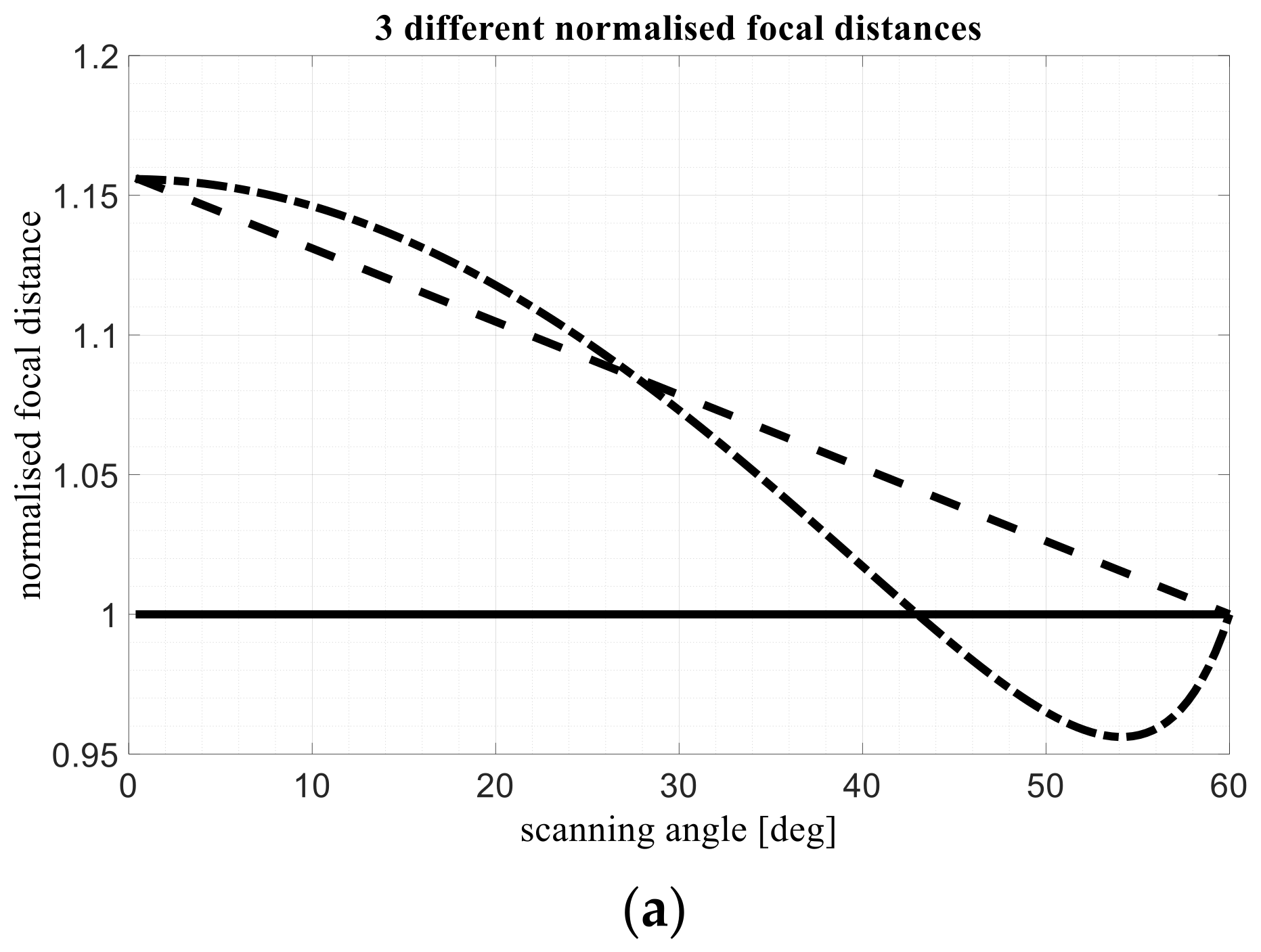
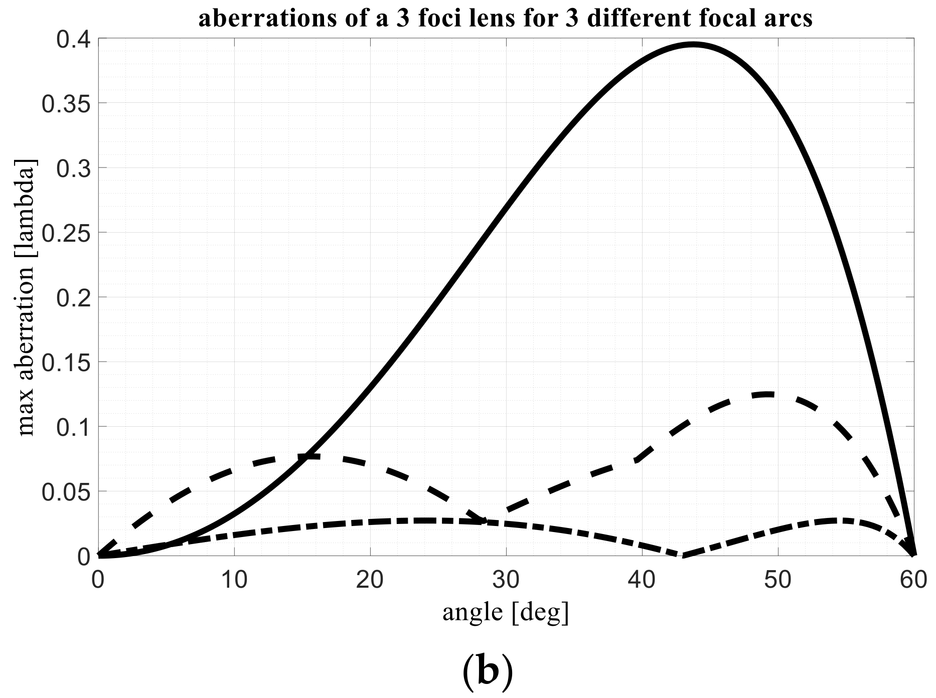
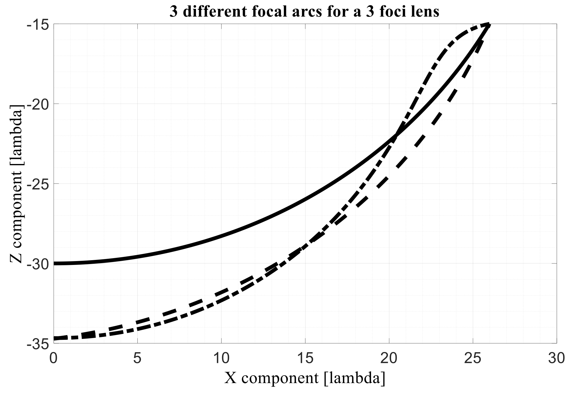
It is important to note that in [16] a 5-foci Rotman lens was proposed. However, it can be easily verified that a discrete lens with a flat front surface cannot guarantee exactly the presence of 5 perfect foci in terms of GO. It is interesting to note that a 5-foci condition can be enforced numerically for a single point of the lens, but a unique lens analytically defined cannot guarantee 5 perfect GO foci for all the points of the lens. The solution proposed here converges to a 5-foci lens architecture for all the points of the lens. As an illustrative example, let us assume a lens characterized by a ratio between the external focal distance F (associated to the maximum scanning angle α) and the diameter D of the front lens unitary: F/D = 1. Let us assume also D = 30 λ, α = 60°. The axial focal length is denoted by G. Three configurations are compared. The first one is such that G = F = 30 λ and for every angle comprised between the extreme angles (−α and +α) the focal distance is assumed to be equal to F = G. In this case, the arc is perfectly circular. The second one is such that the value of G versus F (or, vice versa, F versus G) is given by the heuristic expression (2) presented in Step 1 and, for every angle comprised between the extreme angles (−α and +α), the focal distance is assumed to change linearly as compared to the extreme values F and G. Finally, the third one is such that the value of G versus F (or, vice versa, F versus G) is given again by the heuristic expression presented in Step 1 and, for every angle comprised between the extreme angles (−α and +α), the focal distance is optimized adopting the procedure detailed in the Steps 2 and 3 in order to achieve a Chebyshev envelope for the maximum aberration levels.

In particular, in Figure 2a, the three focal arcs just defined, normalized as compared to F, are represented in a Cartesian representation as a function of the scanning angle. In Figure 2b the maximum aberrations expressed in λ versus the scanning angle are represented. As usually done, for every scanning angle the associated maximum aberration represents the worst value associated to the entire lens. Only half of the scanning angle is considered in Figure 2b because the other half is perfectly symmetric. The curves relevant to the first configuration are black continuous lines; the curves relevant to the second configuration are black dashed lines; the ones relevant to the third configuration are dash-dotted lines. The optimized focal distance in Figure 2a in dash-dotted line exhibits a curved profile. In Figure 3 the same focal arcs are visualized using their X- and Z-components in order to present with a more correct perspective their curvature. It is important to note that the third configuration presents aberrations about 15 times lower as compared to the first one.

Two additional properties can be derived. In correspondence to the angle γ satisfying (1)

sin(γ) ~ (α in radians)/π = (α in degrees)/180

the optimized focal distance has a value which can be estimated using the linear interpolation between the extreme focal distances F and G. This focal distance is already quite well optimized this way as it will be proved later. In correspondence to the angle δ satisfying

sin(δ) ~ (α in radians) 2/π = (α in degrees)/90

(6)

the optimized focal distance has a value similar to F and the aberrations are practically negligible. This angle δ is having a pivotal role in this quasi 5-foci lens design. The tri-focal lens, with initial foci in correspondence to the angle −α, 0 and +α, exhibits at the end of Steps 2 and 3 two additional quasi perfect foci in correspondence of the angles −δ and +δ. For α = π/4 from the previous equations one derives: δ = π/6 = 2/3α and γ ~ π/12. The sinus of the angles γ and δ are related by a simple factor equal to 2.

5. Optimization of 4-Foci Lenses

Let us consider now a two-dimensional discrete 4-foci lens, with a flat profile, 4 identical focal distances, focal points associated with the opening angles −α, −δ, +δ, +α (with δ < α). As anticipated in Section 3, it is simple to verify that the four focal distances associated to the four focal points must be identical, otherwise the 4-foci lens with flat front profile would not be satisfying the 4 GO equations associated with the path lengths. The first challenge in the design of this bootlace lens is the derivation of the ideal position of the two internal foci characterized by the angle δ as compared to the positions of the two external ones, characterized by the angle α, assumed fixed. Any choice is allowed for δ but only one choice guarantees minimized optical aberrations. The second challenge is the derivation of the optimal focal arc.

Step 1:

Estimation of the internal angle δ.

The equation derived in the previous section for the angle δ can be used.

Step 2:

Estimation of the focal arc.

For every generic pointing direction, ranging from 0 to α, the local focal distance is derived enforcing that the aberrations associated to the two extreme points of the lens, i.e., the ones characterized by a minimum and maximum value for the transversal coordinate X1 (and X), be equal in terms of modulus and opposite in terms of sign. This step coincides with the Step 2 proposed for the 3-foci lens. By solving a third-degree equation, the local focal distance can be estimated in an analytical form (see Step 2 of the design for the 3-foci lens).

Step 3:

Iterative refinement.

The previous step 1 is repeated iteratively, adopting a gradient-like algorithm. The internal angle δ is slightly modified in order to minimize the maximum aberrations in the entire field of view and to guarantee a Chebyshev equi-ripple profile for the maximum aberrations versus the scanning angle. As done for the 3-foci lens, an efficient way to speed the convergence consists in choosing as local error the difference between the two local maxima in the absolute value of the aberrations. These two local maxima are located approximately in the angles γ1 an γ2:

sin(γ1) ~ (α in radians)/π,

sin(γ2) ~ [(α in radians) 2/π + sin(α)]/2.

(7)

The iterative procedure can be considered completed when the differences between the two local maxima in the aberrations tend to zero and become smaller as compared to an assigned threshold. In this condition, quasi equi-ripples are obtained (a Chebyshev-like shape for the optical aberrations). The two-dimensional discrete lens antenna with 4 focal points, after applying Steps from 1 to 3, exhibits minimum aberrations with an equi-ripple shape and exhibits quasi 5 focal points. The additional quasi focal point is located in the lens axis. The optimized internal angle δ also satisfies the empirical Equation (6) identified for the 3-foci lens, i.e.:

sin(δ) ~ (α in radians) 2/π = (α in degrees)/90

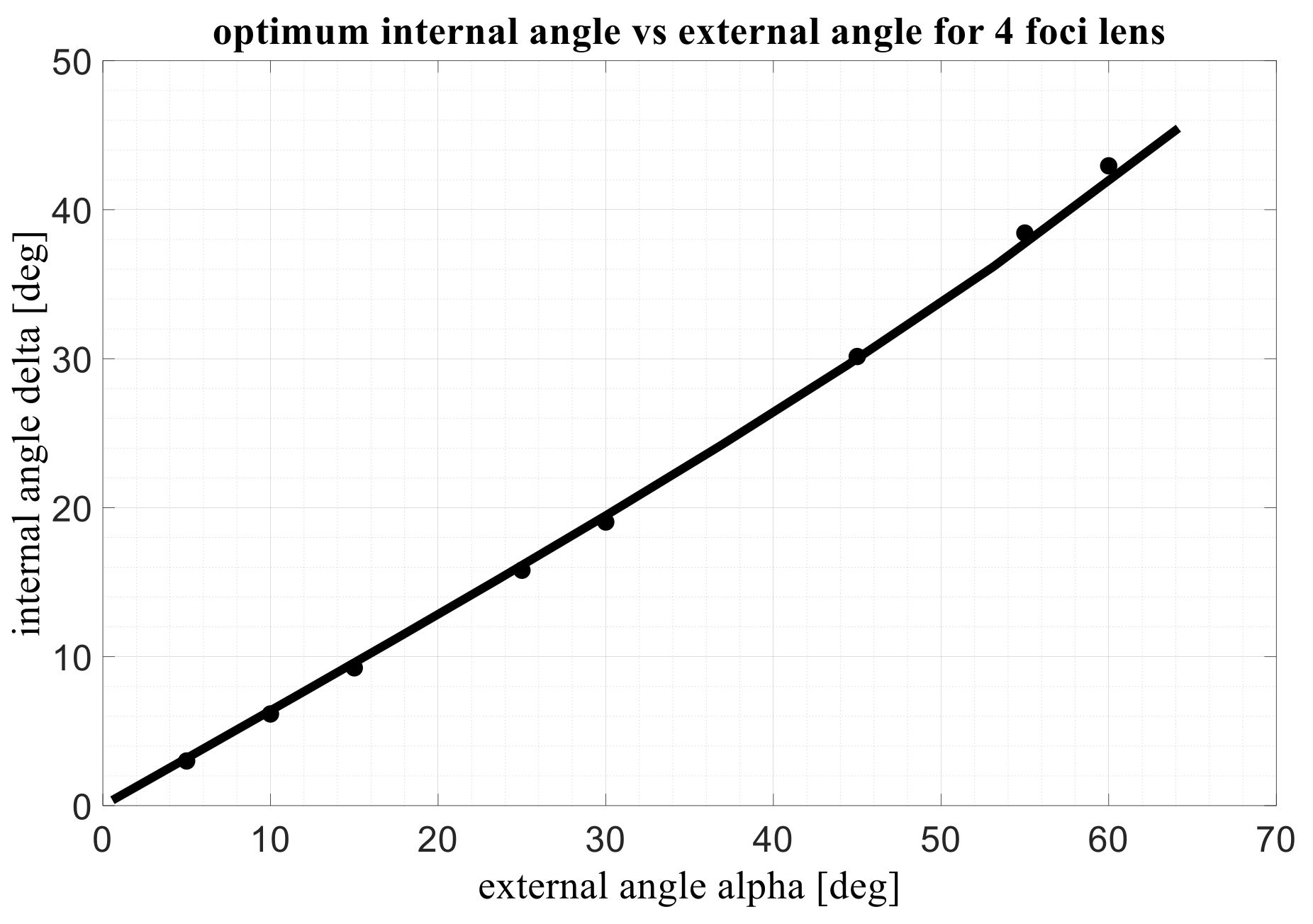
For α = π/4, the heuristic equation gives an internal angle exactly equal to π/3 which seems particularly accurate. In Figure 4, the optimized internal angle δ in the 4-foci lens is plotted as compared to the external angle: the dots represent the numerical optimized values, the black continuous line the new proposed interpolating heuristic curve. It has been verified numerically that similar results in terms of optical aberrations and focal arc shape can be obtained when the design considers as starting point: (a) a 3-foci lens with flat front profile, fixed external angle, fixed value for the external focal distance, fixed diameter for the lens; (b) a 3-foci lens with flat front profile, fixed external angle, fixed value for the axial focal distance, fixed diameter for the lens; (c) a 4-foci lens with flat front profile, fixed external angle, fixed identical value for the 4 focal distances, fixed diameter for the lens.

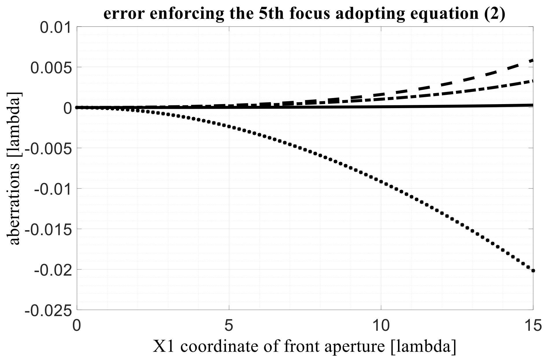
In order to estimate the accuracy of the 5th focus in a 4-foci lens designed with this procedure, let us consider a 4-foci lens with a focal distance F = 30 λ. The $\mathsf{\alpha }$ angle is assuming four possible values, 15°, 30°, 45°, 60°; the magnification factor M = 1, the diameter of the front lens is equal to F. With these inputs, the X, W, Z variables can be derived using the analytical equations of the 4-foci lens. The internal angle of the 4-foci lens is estimated using (6).

Adopting also (2) to approximate G as a function of F, the errors on the lens surface illuminated by the 5th quasi focus located on the lens axis in the point (0, −G) are derived for the 4 values of the $\mathsf{\alpha }$ angle and are plotted in Figure 5. In particular, the continuous line refers to the lens with $\mathsf{\alpha }$ = 15°, the dotted-dashed line to the case with $\mathsf{\alpha }$ = 30°, the dashed line to $\mathsf{\alpha }$ = 45°, and the dotted line to $\mathsf{\alpha }$ = 60°.

It is important to note that these errors are evaluated at the beginning of the design procedure. At the end of the design procedure the residual errors are 3–4 orders of magnitude smaller. In fact, just as an example, for $\mathsf{\alpha }$ = 0.987 radians, using the following equation to link F and G:

$$\mathrm{F}=\mathrm{G}\left(\mathsf{\alpha }-\frac{{\mathsf{\alpha }}^3}{6}-\frac{{\mathsf{\alpha }}^5}{12}+\frac{{\mathsf{\alpha }}^7}{454.3}\right)/\sin \left(\mathsf{\alpha }\right)$$

instead of (2), the maximum error at the edge of the same aperture is ~7.36 × 10⁻⁷ λ.

6. Numerical Results

In this section the 3-foci and 4-foci lenses optimized adopting the procedure discussed in Section 5 are denoted “~5 foci” considering the fact they guarantee quasi 5 perfect foci. Two-dimensional lenses with flat profile can be used to scan beams up to approximately 45–50° (in case M = 1 and the focal lengths are comparable with the lens diameter). Examples with scanning angle $\mathsf{\alpha }$ equal to 60° are presented as well in this section, although they exhibit poor illumination efficiency, i.e., the orientation of the last feeds in the focal arc as compared to the orientation of the back lens elements is significantly skewed.

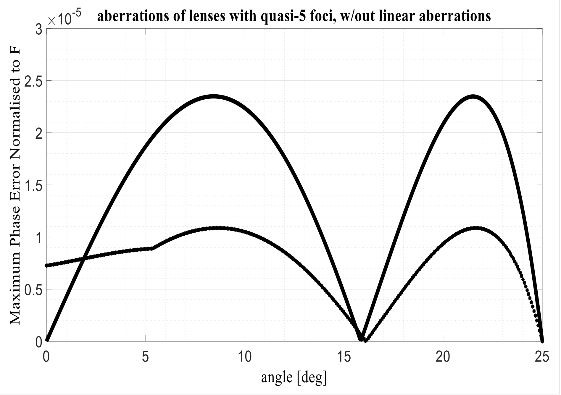
A comparison is proposed, first of all, with the results obtained in [17] where a numerical procedure to optimize a bootlace lens without focal points, i.e., an afocal lens, has been implemented. In particular, in Figure 6 in [17] an afocal lens has been compared in terms of aberrations with a lens characterized by 3 foci, and with a second lens with 4 foci. The three lenses have a planar front profile. These results seem correct; however, the 3 foci and 4 foci lenses presented have not been sufficiently optimized and for this reason, based on our results, they present inferior performance in terms of aberrations as compared to the numerically optimized afocal lens. We have been considering the same configuration obtaining an improvement in terms of aberrations of about one order of magnitude. The results in Figure 6 can be directly compared with the results in Figure 6 in [17]. The upper line presents the aberrations derived when applying the procedure presented in the previous sections. A further reduction in the aberrations can be obtained, after the optimization of the lens parameters and the focal arc, by removing the linear aberrations. Removing the linear aberrations simply implies a minor tuning of the local orientation of the generic feed in the focal arc as compared to the direction of correspondingly generated plane wave possibly considering the magnification factor M. The lower line in Figure 6 presents the aberrations after removing the linear aberrations. As it is evident, this minor correction guarantees a further significant decrease in the maximum aberrations (usually, as confirmed in other examples later, about 50% of improvement in the maximum value of the aberrations can be obtained). When comparing the aberrations achieved with a 4-foci lens in Figure 6 with the 4 foci lens presented in [17], an improvement factor of about 10 is visible. Both lenses are characterized by $\mathsf{\alpha }$ = 25°; however, in Figure 6, the internal angle seems exactly half as compared to the external one, while in the new 4-foci lens proposed here the internal angle has a value around 16° in line with Equation (6). With the new procedure, choosing the angle $\mathsf{\alpha }$ = 25°, the maximum aberrations normalized to F (without linear aberrations compensation) assume the value 2.3866 × 10⁻⁵. After this comparison, one may conclude that the 3- and 4-foci lenses considered in [17] have been only partially optimized. Therefore, the conclusion that the afocal lens outperforms the performances achievable with multifocal lenses does not seem correct. In facts, the ~5 foci constrained lenses proposed here permit to improve significantly the results previously published.

The performance of the ~5-foci lenses are presented in

Table 1. Max aberrations [in λ] ^vs max scanning angle for different F/D (to have them in degrees a 360 factor is required). M = zoom = 1; D = 30 λ.

	F/D = 0.75	F/D = 1	F/D = 1.25	F/D = 1.5	F/D = 2	Q for F/D = 0.75	Q for F/D = 1.25	Q for F/D = 1.5	Q for F/D = 2
α = 60°		0.0271	0.0163	0.011			1.064	1.095
α = 55°		0.021	0.0124	0.0083			1.083	1.124
α = 50°		0.0149	0.0088	0.0058			1.083	1.142
α = 45°		0.0098	0.0058	0.0038	0.0021		1.083	1.157	1.166
α = 40°		0.0061	0.0035	0.0023			1.115	1.178
α = 35°		0.0034	0.0019	0.0013			1.145	1.162
α = 30°		0.0017	9.584 × 10−4	6.33 × 10−4	3.4 × 10−4		1.135	1.192	1.232
α = 25°		7.16 × 10−4	4.126 × 10−4	2.67 × 10−4			1.11	1.188
α = 20°	5.647 × 10−4	2.46 × 10−4	1.422 × 10−4	9.14 × 10−5		1.29	1.107	1.195
α = 15°	1.401 × 10−4	5.94 × 10−5	3.521 × 10−5	2.24 × 10−5	1.23 × 10−5	1.32	1.08	1.177	1.207
α = 10°	1.902 × 10−5	8.39 × 10−6	4.805 × 10−6	3.04 × 10−6		1.274	1.118	1.224
α = 5°	6.058 × 10−7	2.73 × 10−7	1.547 × 10−7	9.81 × 10−8		1.247	1.129	1.235

as a function of the F/D ratio, i.e., the ratio between the focal distance and the lens diameter. In particular, F coincides with the focal used in the definition of both the 3- and 4-foci lenses; D represents the diameter of the front lens aperture. The magnification factor M, or zooming factor, is assumed to be unitary for the time being. In Table 1, lenses with a diameter of 30 λ are considered. In the first column, the value of the external angle $\mathsf{\alpha }$ of the lens defining the maximum scanning angle is defined. In columns 2–6, the maximum aberrations are reported for values of F/D ranging from 0.75 to 2. The diameter of the front lens is considered fixed. Thus, when changing F/D, only the focal distances are scaled and the aberrations change according to this heuristic expression:

Aberrations (F/D = Ω) = Aberration (F/D = 1) Ω² Q

(8)

where Q ranges from about 1.05 (for large angles, i.e., α close to 60°), to 1.25 (for small angles, i.e., $\mathsf{\alpha }$ close to 0°). The Q factors derived empirically are reported in Table 1, in columns 7–10. As evident in (8), aberrations change in quadratic way as a function of the F/D = Ω parameter. After evaluating the effects of the F/D ratio, two additional variations are considered: the evolutions of the optical aberrations as a function of the lens dimensions, and as a function of the magnification or zooming factor M.

Maintaining F/D = 1 and M = 1, when the F = D is changed, the aberrations change linearly, i.e., per F = D = 60 λ all the aberrations double as compared to the case with F = D = 30 λ considered in Table 1.

By fixing the diameter of the front lens, when changing the zooming or magnification factor, the aberrations change linearly as well: for M = 0.5 the maximum aberrations are half as compared to the case with M = 1, when M = 2 the maximum aberrations are double as compared to the case with M = 1.

Considering the three properties just described and the numerical results for the case with F/D = 1, the aberrations associated to discrete two-dimensional lenses with any dimension, magnification, and F/D parameter can be estimated starting from the numerical results presented in Table 1.

It is of interest to compare as well the ~5-foci lens with other two lenses defined in Section 3: the one with a single focal point and the one with two symmetric focal points. It has been observed that despite to the differences between these two lenses with 1 and 2 foci, the corresponding focal arcs, optimized with the general procedure detailed in the Appendix A, tend to be extremely similar. For this reason, an average between the two lenses has been considered as well. An example is presented in

Table 2. Comparison between maximum aberrations of lenses with 1, 2, ~5 foci. F/D = 1, M = 1; D = 30 λ.

	~5 foci	1 focus	2 foci	Average 1 vs. 2 foci
α = 60°	0.0271	0.0825	0.0693	0.0765
α = 45°	0.0098	0.0426	0.0311	0.0366
α = 30°	0.0017	0.0167	0.0108	0.0138
α = 15°	5.945 × 10−5	0.0036	0.0023	0.0029

with F/D = 1, M = 1; D = 30 λ. Only the maximum aberration value is reported.

In

Table 3. F/D = 1, M = 1; D = 30λ.

	Aberrations for lenses with 1 (dash-dotted line), 2 (small squares), and ~5 foci (continuous line). Also the average between the lens with 1 and 2 foci is shown (large rhomboidal dots)	Aberrations of the ~5 foci lens w/out linear aberration compensation. Continuous line: with linear aberrations; dotted line: without linear aberrations.	Angular repointing to remove the linear aberrations. Continuous line: 4-foci lens, dotted line: 3-foci lens.
α = 15°
α = 30°
α = 45°
α = 60°

, the same example is considered. In the first column, the angle defining the maximum scanning of the lens is defined. In the second column, the evolutions of the aberrations with respect to the scanning angle are reported. In the third column, the aberrations for the ~5-foci lens are plotted with and without the contribution of the linear aberrations. Finally, in the fourth column, the angular repointing needed to remove the linear aberrations is shown. It is quite interesting to note that a local repointing of the feed by an angle which is a small fraction of 1° (i.e., from 10⁻³ to 10⁻⁶ degrees!) can have such a significant impact on the aberrations’ evolution. Four opening angles α ranging from 15° to 60° are considered. The lens with a single focus (dash-dotted line), as expected, permits to control the aberrations only close to the axial direction and aberrations increase when scanning. The lens with two foci (small square points) permits to perfectly cancel the aberrations in two symmetric angles but its aberrations worsen when approaching the lens axis. The configuration average between the 1- and 2-foci lenses (large rhomboidal points) presents intermediate results. The continuous line refers to the ~5-foci lens. For low values of α, the ~5-foci lens performs much better. For α approaching 60°, the performance is comparable up to a certain angle. However, for angles approaching α, the ~5-foci lens remains significantly better because is able to perfectly cancel the aberrations in α.

Table 4. Maximum aberrations normalized to the focal distance for discrete lenses having F/D = 1, M = 1 and ~5 foci.

α = 60°	9.033 × 10−4
α = 55°	0.0007
α = 50°	4.96 × 10−4
α = 45°	3.26 × 10−4
α = 40°	2.03 × 10−4
α = 35°	1.13 × 10−4
α = 30°	5.66 × 10−5
α = 25°	2.38 × 10−5
α = 20°	0.82 × 10−5
α = 15°	1.98 × 10−6
α = 10°	2.79 × 10−7
α = 5°	9.10 × 10−9

reports the maximum aberrations normalized to the focal distance for discrete lenses having F/D = 1 and M = 1.

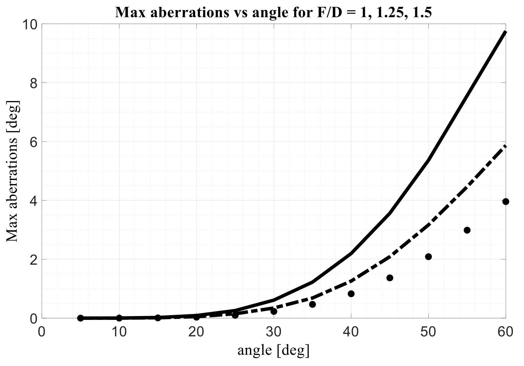
In Figure 7, the maximum aberrations, expressed in degrees, as a function of the maximum scanning angle, in degrees, for three different values of the F/D, are plotted. The diameter of the front lens is again fixed to 30 λ. The continuous curve refers to the case F/D = 1; the dashed curve is valid for F/D = 1.25 while the dotted curve for F/D = 1.5. As expected, the aberrations increase with the scanning angle and by reducing the F/D value.

Removing the linear aberrations, a further improvement can be obtained in the maximum value of the aberrations.

In

Table 5. Aberrations and lateral focal distance for lenses having h/D = 10/3, M = 1.

h = 10 λ D = 3 λ	$\mathrm{F}=\mathrm{G}\left(\mathsf{\alpha }-\frac{{\mathsf{\alpha }}^3}{6}-\frac{{\mathsf{\alpha }}^5}{12}\right)/ \sin \left(\mathsf{\alpha }\right)$	Max aberration [λ] D = G 0.3
α = 75°	F = G 0.65533	max aberration = 7.4 × 10−4
α = 60°	F = G 0.87359	max aberration = 2.8 × 10−4
α = 45°	F = G 0.96196	max aberration < 7.85 × 10−5
α = 30°	F = G 0.99269	max aberration < 1.2 × 10−5
α = 15°	F = G 0.99955	max aberration = 4.1 × 10−7
α = 5°	F = G 0.99999	max aberration = 8 × 10−9

, a configuration with the axial focal distance h = 10 λ and D = 3 λ is considered. The magnification factor M = 1. The optimized values for the maximum aberration and the lateral focal distances F are reported.

Another example with a lens having a diameter D = 10 λ is reported in

Table 6. Aberrations and Q factors for lenses with M = 1; D = 10 λ-.

	Aberrations for ~5 foci, F/D = 1	Aberrations for ~5 foci, F/D = 1.5	Aberrations for ~5 foci, F/D = 2	Factor Q (see (8)), for F/D = 1. 5	Factor Q (see (8)), for F/D = 2
α = 60°	0.009	0.0037	0.0021	1.081	1.071
α = 45°	0.0033	0.0013	0.000694	1.128	1.188
α = 30°	5.5 × 10−4	2.1 × 10−4	1.15 × 10−4	1.144	1.199
α = 15°	1.9 × 10−5	7.7 × 10−6	4.1 × 10−6	1.191	1.202

. The magnification factor M = 1. The reported Q factors, numerically estimated, are well in line with the values predicted with the heuristic Equation (8) that becomes this way validated also for electrically small lenses.

Additionally, a visual comparison with the R-2R lens is of interest. In

Table 7. Focal arc vs. back lens profile vs. circular shapes F/D = 1, zoom = 1, D = 30λ-.

α = 15°		α = 30°
α = 45°		α = 60°

, the back profile of ~5-foci lenses (the front is simply flat) and the profile of the corresponding optimized focal arc are represented by thick black lines. The thin dotted lines represented portions of circles characterized by a radius equal to G or G/2 and centered in the point (0,0), (0,−G/2), (0,−G).

It is also known that the R-2R has a back profile coinciding with a circle of radius G/2 and centered in the point (0,−G/2). The focal arc is defined in the opposite part of the same circle. The front profile for the R-2R lens coincides with a circle of radius centered in the point (0,−G).

Three asymptotic properties can be observed. First of all, the back profile of the ~5-foci lenses optimized with the procedure detailed in the paper, can be approximated by a portion of a circle centered in the point (0, −$\frac{\mathrm{F}}{2}\frac{1}{\cos \left(\mathsf{\alpha }\mathsf{\delta }\_\mathrm{average}\right)}$) and with a radius equal to:

$$r_{back\_asympt}=\frac{\mathrm{F}}{2}\frac{1}{\cos \left(\mathsf{\alpha }\mathsf{\delta }\_\mathrm{average}\right)}$$

(9)

where $\mathsf{\alpha }\mathsf{\delta }\_\mathrm{average}$ defines the average between the two angles $\mathsf{\alpha }$ and $\mathsf{\delta }$ defining the external and internal foci in the ~5-foci lens. Second, the focal curve of the ~5-foci lenses can be approximated by a portion of a circle centered in the point (0,−(G − G $\cos \left(\mathsf{\alpha }\mathsf{\delta }\_\mathrm{average}\right)$) and with a radius equal to:

$$r_{focal\_asympt}=\mathrm{G}\cos \left(\mathsf{\alpha }\mathsf{\delta }\_\mathrm{average}\right)$$

(10)

The two asymptotic circles are also drawn in Table 7 with thin lines while the thick lines refer to the back profile and focal curve derived rigorously. The first asymptotic property on the back array shape is particularly accurate. One third property concerns the shape of the focal arc and back profile for small values of the α angle. As evident in Table 7, for small α angles the shape of the focal arc is well approximated by a portion of the circle with radius G and centered in the (0,0) point. The shape of the back lenses, always for small values of the α angle, is well approximated by a circle of radius G/2 (in line also with the previous equation considering $\cos \left(\mathsf{\delta }\right)1$). Therefore, for small α angles the ~5 foci can be considered a 2R-R-0 lens because the focal arc is similar to a circle of radius 2R = G, the back lens is similar to a circle of radius R = G/2, while the front profile is flat.

7. Conclusions: Summarizing the Properties of Two-Dimensional Bootlace Lenses with Flat Front Profile

Two-dimensional bootlace constrained lenses with flat profile with one, two, three or four perfect foci can be defined analytically in explicit form (see Section 3). The R-2R lens exhibits an infinite number of foci but its front profile is circular.

A five-foci bootlace lens with a flat profile cannot be defined analytically adopting the GO ray tracing law. It is possible to enforce numerically five focal points when considering a single point on the lens. However, when considering a different point and enforcing again the same five foci, the numerically derived lens parameters change. This means that a bootlace lens satisfying the five perfect foci conditions for all the lens is not existing.

A two-dimensional discrete lens with ~5 foci (quasi-5 foci) featuring minimum optical aberrations has been presented. The same identical configuration can be obtained adopting as starting points two completely different lens architectures: a 3-foci lens with an axial focus and 2 symmetrical ones, and a 4-foci lens with two couples of symmetrical foci. The ~5-foci lens exhibits Chebyshev-like equi-ripple minimized aberrations.

The analytical relation between the two focal distances of the 3-foci lens has been derived heuristically in (2). The angle defining the additional couple of foci in the 3-foci lens coinciding with the position of the internal couple of foci in the 4-foci lens has been estimated heuristically in (6). An analytical expression for the focal distance associated to a generic incidence angle has been found by solving a third degree equation. Simplifications for this expression have been proposed. A second more accurate but indirect way to derive an optimum value for G as a function of F, consists in optimizing first a 4-foci lens so finding for δ an improved value as compared to the one defined in (6). At this point X, W, and Z are known together with F and δ. By solving now in G the GO equation which guarantees an additional focus in the lens axis in the point (−G,0) this value is found:

$$\mathrm{G}=-\left({\mathrm{X}}^2+{\mathrm{Z}}^2-{\mathrm{W}}^2\right)/\left(2\mathrm{W}+2\mathrm{Z}\right)$$

(11)

As G should assume a single real value, G can be estimated with (11) by adopting for X, W and Z their value in a single point possibly in the vicinity of the edge of the lens where a single axial focus generates maximum aberrations. The values found for G in this way provide really low aberrations.

It is important to note that in case of magnification (i.e., zooming) different from 1, the same equations remain valid.

It has been verified that by slightly modifying the ~5-foci configuration identified, the aberrations become worse, i.e., one of the two equi-ripple lobes becomes higher while the other one becomes lower, so, overall, the maximum aberration associated with the lens becomes worse. Therefore, the derived solution is locally optimal.

Some advantages of the 4-foci lens have been identified as compared to the 3-foci lens: (1) the optimized values for the 4 focal distances are already known a priori (being identical) while for the 3-foci lens the relation between F and G is not known in advance; (2) the profile of the 4-foci lens is a simple parabolic profile (although this property is true when representing Z as a function of X1 and not X), while for the 3-foci lens the profile is given in terms of a more complex analytical equation involving radicals; (3) starting from the 4-foci lens equations, the presence of a 5th quasi focus (satisfying the GO equi-path condition for one additional feed on the lens axis) can be easily added.

The evolutions of the maximum aberrations as a function of the lens dimensions, F/D ratio and magnification factor M have been estimated. The results contained in the Tables permit the antenna designer to characterize the dimensions and maximum aberrations of an arbitrary two-dimensional lens with a flat profile.

It has been found that removing the linear aberrations permits to approximately half the maximum aberrations independently of the opening angle of the lens $\mathsf{\alpha }$.

The back profile of ~5-foci proposed lenses can be approximated extremely well by a portion of a circle of radius:

$$r_{back\_asympt}=\frac{\mathrm{F}}{2}\frac{1}{\cos \left(\mathsf{\alpha }\mathsf{\delta }\_\mathrm{average}\right)}$$

where $\mathsf{\alpha }\mathsf{\delta }\_\mathrm{average}$ defines the average between the two angles $\mathsf{\alpha }$ and $\mathsf{\delta }$ defining the external and internal foci in the lens.

The focal curve of the ~5-foci lenses can be approximated by a portion of a circle centered in the point (0, −(G − G$\cos \left(\mathsf{\alpha }\mathsf{\delta }\_\mathrm{average}\right)$) and with radius equal to:

$$r_{focal\_asympt}=\mathrm{G}\cos \left(\mathsf{\alpha }\mathsf{\delta }\_\mathrm{average}\right)$$

For small values of the α angle, the shape of the back lenses is well approximated by a circle of radius G/2, and the focal arc is well approximated by a portion of the circle with radius G and centered in the (0,0) point. Thus, for small $\mathsf{\alpha }$ angles, the ~5 foci can be considered a 2R-R-0 lens because the focal arc is similar to a circle of radius 2R = G, the back lens is similar to a circle of radius R = G/2, while the front profile is flat.

It has been discovered that, after defining optimally the focal distances, enforcing opposite values for the aberrations on the two extreme points of the lens represents the fundamental condition to derive analytically a locally optimal focal distance for arbitrary angles. This property applies to lenses such as the 3- and 4-foci ones. For other types of lenses, such as the one with a single focal point, a general procedure to derive the focal arc is proposed in the Appendix A.

Finally, it is important to observe that the analytic solutions for multifocal constrained lenses tend to be extremely ill-conditioned from a mathematical point of view (i.e., the greater the number of foci, the higher the ill-conditioning). This means that small variations in one of the variables defining the lens can justify significant modifications in the optical aberrations. As a consequence, optimizations based on brute force numerical techniques are extremely slow and may result in being completely ineffective.

The design procedure takes into account only the phase response and the associated optical aberrations. The behavior of the amplitude of the field, considering all possible losses and mismatches, is important as well and should be considered in a second part of the design adopting full wave electromagnetic solvers as done in [18,19,20,21].