Zhongshan HF Radar Elevation Calibration Based on Ground Backscatter Echoes

Abstract

The super dual auroral radar network (SuperDARN) is an important tool in the remote sensing of ionospheric potential convection in middle and high latitudes, and also a major source of elevation data detection. A reliable elevation angle helps estimate the propagation paths of high-frequency radio signals between scattering spots and radars, which is crucial for determining high-frequency radar target geolocation. The SuperDARN radar uses interferometry to estimate the elevation of the returned signal. However, elevation data are still underutilized owing to the difficulties of phase difference calibration induced by the propagation time delay between two arrays. This paper statistically analyzes the distribution features of the group range-elevation angle and group range-virtual height before and after calibration using elevation data from the ground backscatter echoes of the Zhongshan SuperDARN radar, calculating the root mean square error (RMSE) of the virtual height; the results show that the RMSE after calibration is mostly reduced to within 54% of that before calibration. Furthermore, we validate the calibration factor based on the primary phase data. The data from 2013 to 2015 indicate that this technique can be efficiently used to estimate the daily calibration factor. Finally, we present the statistical distribution of the calibration factor, which provides technical support for the calibration of elevation data in the future.

1. Introduction

The super dual auroral radar network (SuperDARN) is one of the most essential pieces of equipment for exploring the ionosphere and magnetosphere at high and mid-latitudes [1,2,3]. There are now more than 35 radars running in the world [4,5]. SuperDARN has become a powerful tool for detecting ionospheric plasma convection [6] for its large geographical coverage and high time resolution [7]. Utilizing the field of views (FOVs) velocity information of different radars, an ionospheric convection pattern can be effectively created to sense space weather conditions. 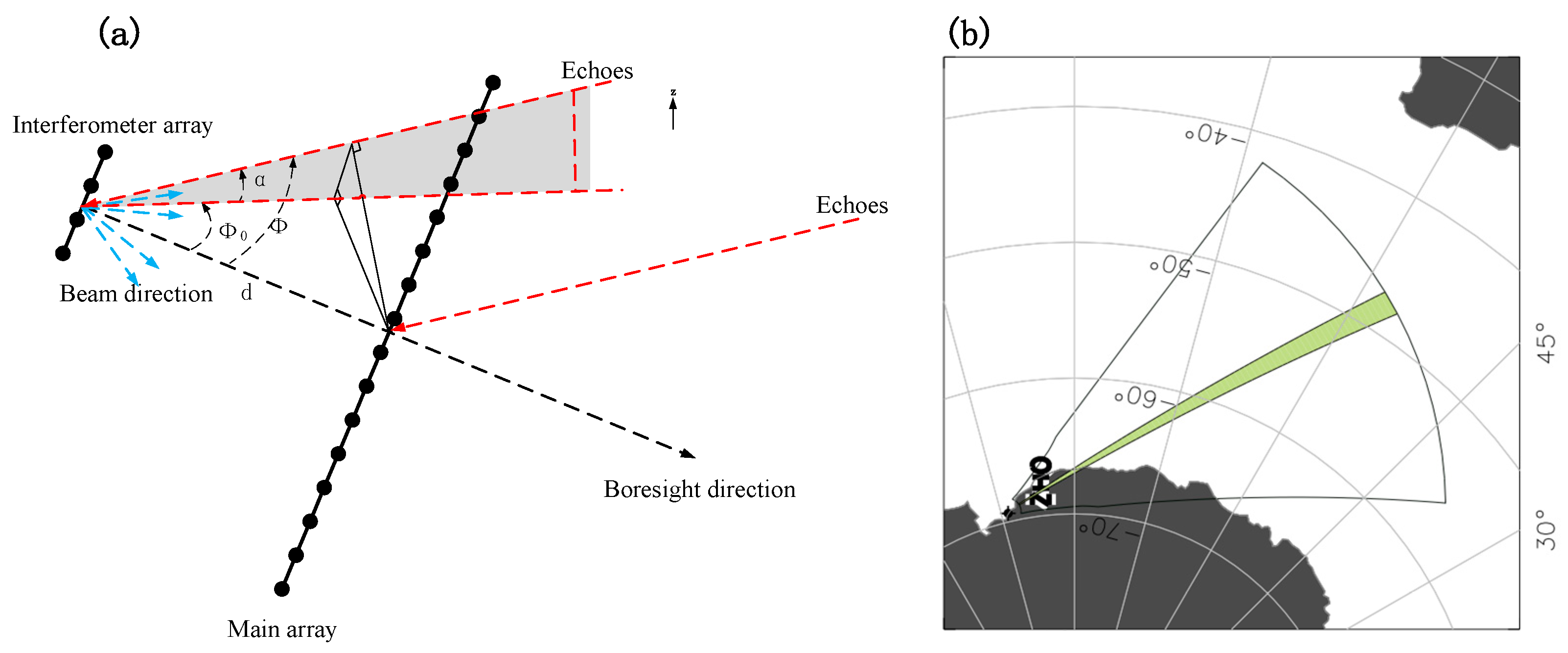Accurate geolocation of radar echoes is a significant basis for the above research [8]. The elevation angle is the main information for the determination of the source of the irregularities, and it is one of the parameters measured by the SuperDARN radar. Many SuperDARN radars are equipped with a main array and interferometer array, and the distance between the two arrays along the radar line of sight is in the order of a hundred meters. For Zhongshan Station, it is about 100 m. The elevation angle is obtained by measuring the phase difference between the received signals of the antenna arrays [1,9]. However, due to the propagation time delay (also known as the calibration factor, $\Delta t_{cor}$) caused by the different propagation paths from the main and auxiliary array to the point at which the return signals from the two arrays are correlated with each other is difficult to be measured, and elevation data have not been fully applied [10].

The adaptive algorithm is widely used in the current radar signal processing design and has a significant effect. To overcome the analytical and numerical difficulties in the optimal approximation of radar detection, a general reduced-complexity algorithm is proposed and analyzed using an adaptive radar detector with desired behavior [11]. The detection of the ionospheric target echoes using wideband radar is also common. Wiener filtering is used to denoise the radar echoes containing noise with the desired signal. Synthetic data and real data verified the effectiveness of the detector [12]. The detection of target echoes by the SuperDARN radar is mainly based on an uncorrelated weighted median filter, which is effective at removing most speckle and Gaussian noise in the echoes [13]. There have been two methods to estimate the $\Delta t_{cor}$ until recently [14]. The first one is to measure the delays of the test signals in the radar cable and the equipment [15]. However, owing to the constraints of the radar geographical location, operating frequency, temperature, or other conditions, these factors cannot be fully controlled, and the dependence between these parameters cannot be evaluated, so we have not considered it. The other one eliminates the influence of the radar hardware itself on the measurement, using elevation data or phase difference data to adjust the $\Delta t_{cor}$, so that the calculated elevation obeys a specific propagation mode or distribution [1]. Recently, with the increasing importance of elevation data, some scholars have concentrated on developing significant calibration techniques based on existing elevation data. For example, an empirical virtual height model for interferometry data by studying the distribution relationship between group range-elevation angle and group range-virtual height [16]; a visual analysis method to detect and calibrate the phase offset in high-frequency interference data [10]; systematically describing the virtual height with each range of near-range SuperDARN meteor echoes is constant over a set time interval [9], or using the low-angle propagation mode and the low variability of the E layer echoes to design an automatic calibration procedure [1]. However, the virtual height model needs to consider the potential effects of time, solar cycles, and beams; in addition, the separation of ionospheric and ground backscatter echoes is difficult [14]. The meteor scatter method has been studied at different temporal resolutions, but the results have not been fully validated [9], and near range meteor echoes can be contaminated by back lobe echoes. The E-region method may cause errors in some periods due to the existence of F echoes. Overall, each of the proposed methods lacks a numerical analysis of the estimated calibration factors and calibrate in an independent way.

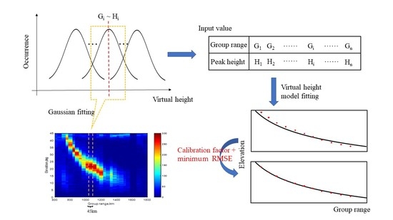
Considering the possible problems of the above methods, this paper aims to improve the previous technology and proposes a new elevation calibration method based on ground backscatter echoes. Based on the virtual height model, this method takes the peak value of Gaussian fitting in each group range of ground echoes as the input and uses the minimum root mean square error criterion as the condition for estimating $\Delta t_{cor}$, which can achieve a high time resolution. The numerical analysis also minimizes the error caused by the visual analysis. The proposed algorithm improves the time resolution of $\Delta t_{cor}$ estimates and verifies, reduces the influence of visual analysis.

The structure of the rest of the paper is as follows. Section 2 briefly introduces the equipment, data set, and the calculation of the elevation angle. Section 3 describes the calibration method of elevation angle. Section 4 presents the discussion of results. Section 5 concludes the paper.

2. Materials and Theories

2.1. Instrumentation and Data

SuperDARN was created in the 1980s [17]. It is an international network of high-frequency (~8–20 MHz) coherent-scatter radars covering the middle and high latitudes of the Northern and Southern hemispheres [9,16,18,19]. Usually, they are composed of a main array and an interference array with a distance of 100 m. The main array comprises 16 antennas for transmitting and receiving signals, and the interference array comprises 4 antennas for receiving signals only [8,20]. The SuperDARN radar takes beam 7 as the boresight direction and uses the “sweeping mode” to scan through 16 uniformly distributed sector areas within ± 26° of the line of sight, which are generally regarded as 16 beams [16,21,22]. Completing a beam scanning takes about 3 s or 6 s, and the whole scan process takes 1 or 2 min [4,23,24]. Each beam starts at a threshold of 180 km from the radar center, with a range gate resolution of 45 km, and can detect group range values of about 3000–5000 km from the radar [25,26]. The parameters of SuperDARN radar detection include backscatter power, line-of-sight Doppler velocity, Doppler spectrum width, and elevation angle.

The data used here are detected by the Zhongshan SuperDARN ground backscatter from 2013 to 2015 in the solar maximum, for which much more backscatter echoes can be received statistically by SuperDARN than for other years. In addition, we excluded the points with an elevation angle of zero in the data set in the preprocessing, which could be invalid scattering points collected by radar hardware. The frequency range of the radar at the Zhongshan radar was 10.2 MHz–10.4 MHz, which is relatively small, so the possible influence of frequency was not in the scope of this paper.

2.2. Elevation Angle Calculation

SuperDARN measures the phase difference between the main and interference arrays for the estimation of the elevation angle. The phase difference measured by the radar is composed of two parts [9]. One part is the phase difference due to the difference in the propagation path of the two antenna arrays when receiving the return signals, ${\Psi }_p$, this is also the ideal state of the radar after calibration. The spatial geometric relationship of the echoes in two antenna arrays is shown in Figure 1. Based on the distribution of space, ${\Psi }_p$, given by

$${\Psi }_p=|\mathrm{k}|d\cos \varphi \cos \alpha$$

(1)

where |k| is the wavenumber, which is actually the amplitude of the wave vector of the backscattered signal, defined as; f and c are the radar frequency and speed of light, respectively; d is the distance between the main and interferometer arrays along the boresight direction; the value at the Zhongshan radar is about 100 m; $\varphi$ is the azimuthal angle of the echoes along the boresight direction; and α is the elevation angle of the signal in the projection direction.

The other part is the unknown phase offset (${\Psi }_{cor}$) caused by the radar hardware time delay; this additional delay is termed the calibration factor ($\Delta t_{cor}$). $\Delta t_{cor}$is caused by the characteristics of the radar instruments, and it cannot be directly determined by a mathematical method, which is the difficulty of calibration for the wide use of SuperDARN. The relationship between ${\Psi }_{cor}$ and $\Delta t_{cor}$ is given by

$${\Psi }_{cor}=-2\pi f\Delta t_{cor}$$

(2)

In addition, the frequency range of the high-frequency radar in the Zhongshan radar is 8–20 MHz [23]. According to the wavelength formula $\lambda =\mathrm{c}/\mathrm{f}$, the distance between the two arrays is greater than the wavelength λ of the transmitted signal (~15–37.5 m). As the measured phase difference is restricted to be between $-\pi$ and $\pi$, there is a potential ambiguity between the measured ($\Psi$) and the actual phase difference [2,15]. This can be seen as the black solid curve and the dashed curve in Figure 2 with $\Delta t_{cor}=-10\mathrm{ns}$. Therefore, the ideal phase difference and the measured phase difference can be rewritten as

$${\Psi }_p=\Psi -{\Psi }_{cor}\pm 2\pi n$$

(3)

Considering that the geometrical relationship between the beam direction, the line-of-sight direction, and the elevation angle is shown in Figure 1, $\varphi 0$ is the azimuth angle of the radar, and the measured elevation angle is correlated with the azimuth angle of the echo signal projection relative to the line-of-sight direction [24], by

$$\sin {\varphi }_0=\sin \varphi \cos \alpha$$

(4)

Following Equation (1), the relationship between the phase difference and the elevation can be defined as

$${\Psi }_p=kd\sqrt{{\cos }^2\alpha -{\sin }^2{\varphi }_0}=kd\sqrt{{\cos }^2{\varphi }_0-{\sin }^2\alpha }$$

(5)

$$\sin \alpha =\sqrt{{\cos }^2{\varphi }_0-\frac{{\Psi }_p^2}{k^2{d}^2}}$$

(6)

From (5) and (6), there is a maximum value for the phase difference and elevation angle. When the maximum value is exceeded, the error caused by ambiguity needs to be solved. ${\Psi }_{\max }$ is observed at a zero elevation angle, given by

$${\Psi }_{\max }=kd\cos {\varphi }_0+{\Psi }_{cor}$$

(7)

The actual phase of the radar processed by Equation (3) is in the range indicated by the black or red horizontal dotted line in Figure 2. The radar main array used in this paper is located in front of the interference array, so the actual phase difference should be satisfied

$${\Psi }_{\max }-2\pi <{\Psi }_p\le {\Psi }_{\max }$$

(8)

Therefore, the elevation angle of the received signal should be smaller than the value of that when ${\Psi }_p={\Psi }_{\max }-2\pi$, that is, the maximum elevation angle given by

$${\alpha }_{\max }=\arcsin \sqrt{\frac{4\pi }{kd}\cos {\varphi }_0-{(\frac{2\pi }{kd})}^2}$$

(9)

Hence, ${\alpha }_{\max }$ varies with the distance between the two arrays, the wavenumber, and the azimuth angle corresponding to the beam $\varphi 0$. The black and red vertical dashed lines in Figure 2 show a difference of about 3° in the ${\alpha }_{\max }$ between the central beam and the edge beam.

3. Method

The calibration of the elevation angle is the estimation of the phase offset. First, it is necessary to determine the expected propagation mode of the elevation angle [10]. For backscatter echoes of the same type, the virtual height reflected by the ionosphere at different group ranges is thought to be constant. That is, the elevation angle measured by the radar should show a nonlinear downward trend with the increase in group range until the elevation angle value approaches zero. According to the basic theory of radio wave propagation, the virtual height is calculated as

$$h=\sqrt{R^2+r^2+2rR\sin \alpha }-R$$

(10)

where R is the radius of the Earth, generally, 6371 km, and r is the group range, that is, the distance from the ionospheric reflection point to the radar station (assuming that the spatial shape of the reflection point to the radar and the scattering point is symmetrical).

In this paper, the root means square error (RMSE) is used as the performance index to evaluate $\Delta t_{cor}$. By tuning $\Delta t_{cor}$ to make the RMSE between the distribution of the virtual height and the curve defined by Equation (10) at a minimum, then the best fitting virtual height is selected and the validity of $\Delta t_{cor}$ is verified by the virtual height and the original phase data. The previous method selects the group range–elevation angle or group range–phase deviation as a single consideration factor to calibrate the additional phase offset generated by the radar hardware according to the expected change of the low-angle echoes characteristics. However, the error of a single data point can only be verified and excluded by another large amount of data. The technique proposed here can not only eliminate the estimation error of $\Delta t_{cor}$, but also increase the stability of $\Delta t_{cor}$ through the mean value in a large time range.

When selecting the optimal $\Delta t_{cor}$, the virtual height is used as an assessment parameter. The theoretical virtual height with the group range should be in as small of a range as possible, and the distribution of the elevation angle should be consistent with the fitting curve of the virtual height. To quantitatively complete the calculation, the RMSE of the virtual height is calculated using the fitting curve, and the maximum point of Gaussian fitting of the elevation distribution in a range gate is used. The RMSE defined as

$${\mathrm{V}}_{cor}=\sqrt{[{\displaystyle \sum _{i=1}^n(h_i-H_{fit})^2}]/n}$$

(11)

$H_{fit}$ is the fitting virtual height based on the peak value of the elevation angle within each range gate, n is the gate number, and $h_i$ is the virtual height calculated by the actual elevation angle.

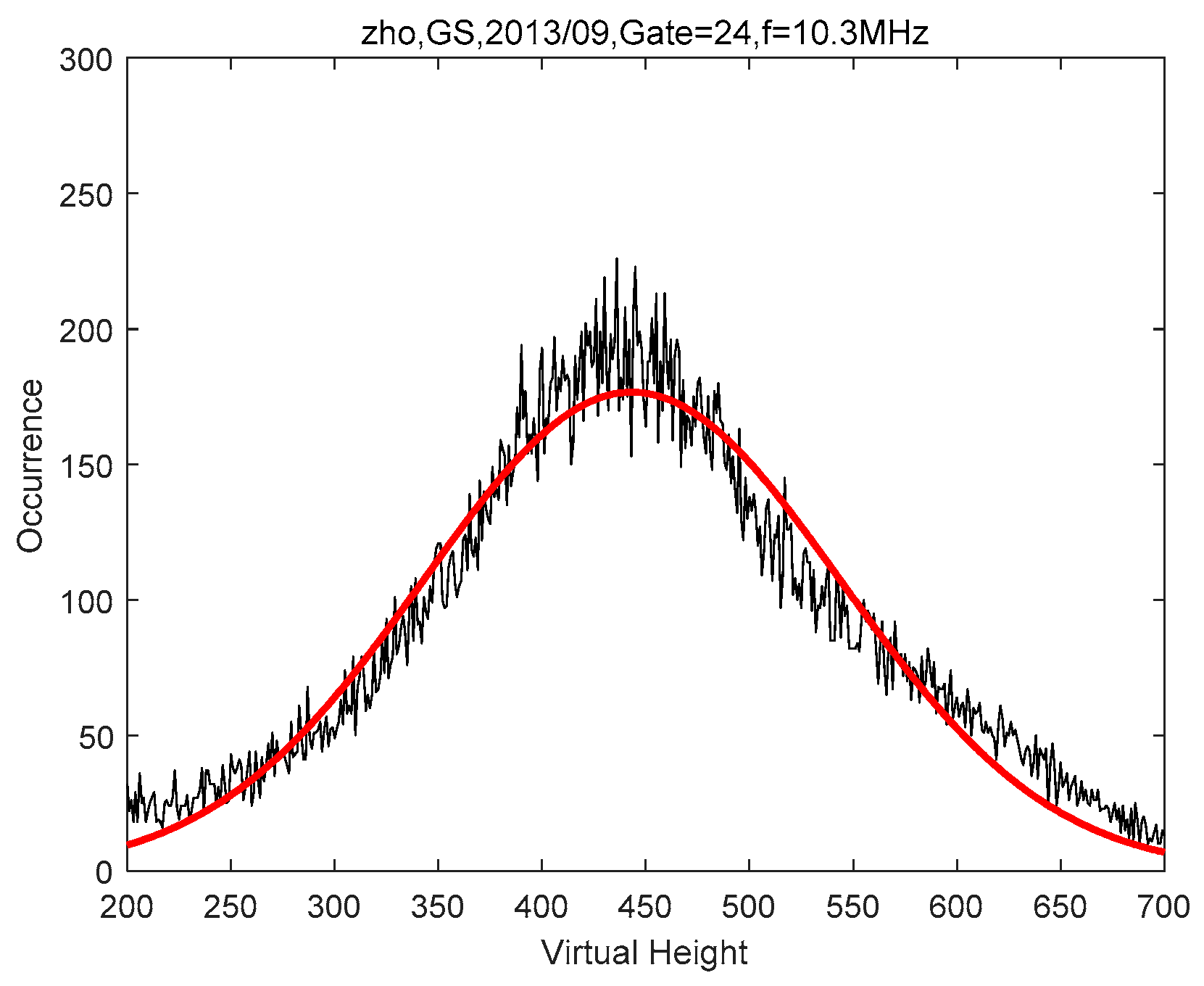
The method involves combining the visual analysis and numerical analysis by gradually adjusting the value of the calibration factor $\Delta t_{cor}$ (the resolution of $\Delta t_{cor}$ is 0.1 ns) to minimize the RMSE of the peak height on each range gate. The range gate distributions for the ground backscatter echoes of the Zhongshan radar are from 15 to 35. For the elevation distribution of one gate, the corresponding virtual height is close to the Gaussian distribution, as shown in Figure 3, the peak value of Gaussian fitting is different in different group ranges, and the value of $\Delta t_{cor}$ will be selected when the RMSE of the virtual height under different group ranges tends to be minimum. 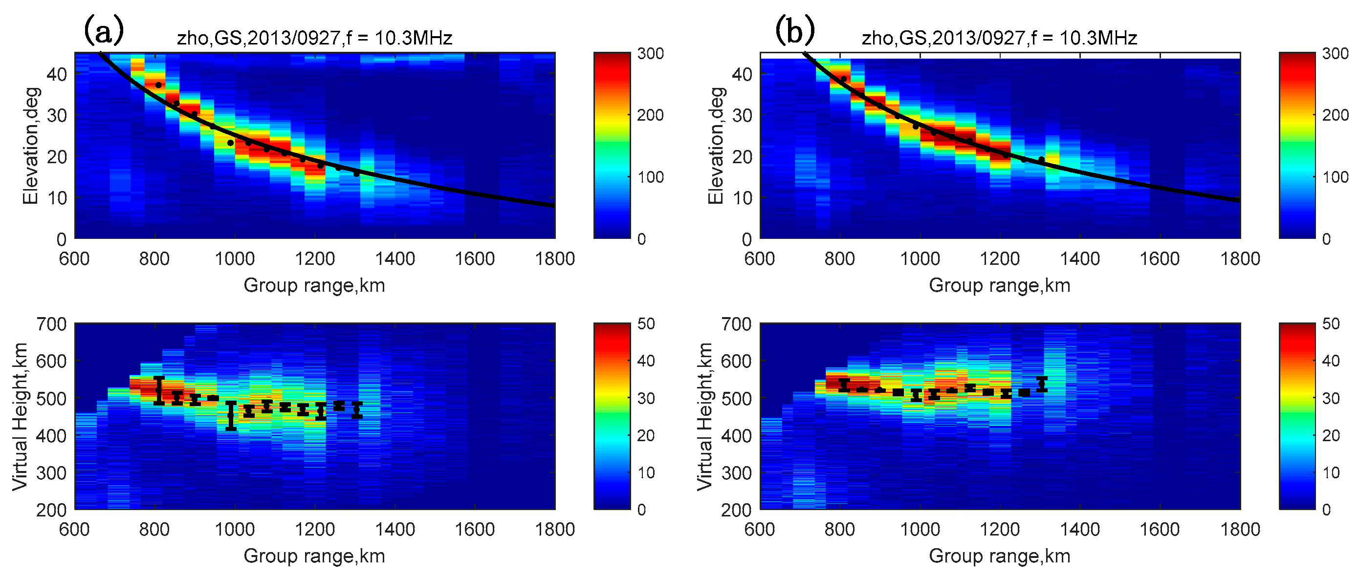An example of the ground backscatter of the Zhongshan radar in September 2013 from the methodology to determine $\Delta t_{cor}$ is presented in Figure 4. The top of Figure 4a shows the distribution of the group range–elevation angle of the original data and the fitting lines according to Equation (10). There is a clear nonlinear relationship between the elevation angle and the group range in the range gate of 15–30 (corresponding to the group range of 810–1485 km). The black dots represent the maximum occurrence in each gate, and the black solid lines show the fitted virtual heights based on these points. At the fixed virtual height, the peak point of the original data cannot match the trend of the fitting curve well, the virtual height distribution of different group ranges is in a large scope, error bars in the bottom of Figure 4a show the deviations in virtual height for each gate with an overall smaller change compared with the bottom of Figure 4b, and a significant difference in peak height in the group range between 800 and 1000 km. When determining the calibration factor $\Delta t_{cor}$, we use intervals of 0.1 ns in the range of −10~10 ns to identify the value of $\Delta t_{cor}$. Figure 4b shows the trend of the elevation angle and virtual height of the minimum RMSE with a value of $\Delta t_{cor}$ is −6 ns. The calibrated elevation angle coincides with the standard curve, the fluctuation of the virtual height with the group range is more concentrated, and the overall error bars decrease. According to Equation (11), the RMSE before calibration is 18.38 km while after it is 10.2 km. The calibrated virtual height of the ground backscatter echoes is 520 km. The distribution of the virtual height determined by RMSE shows good results in the calibration.

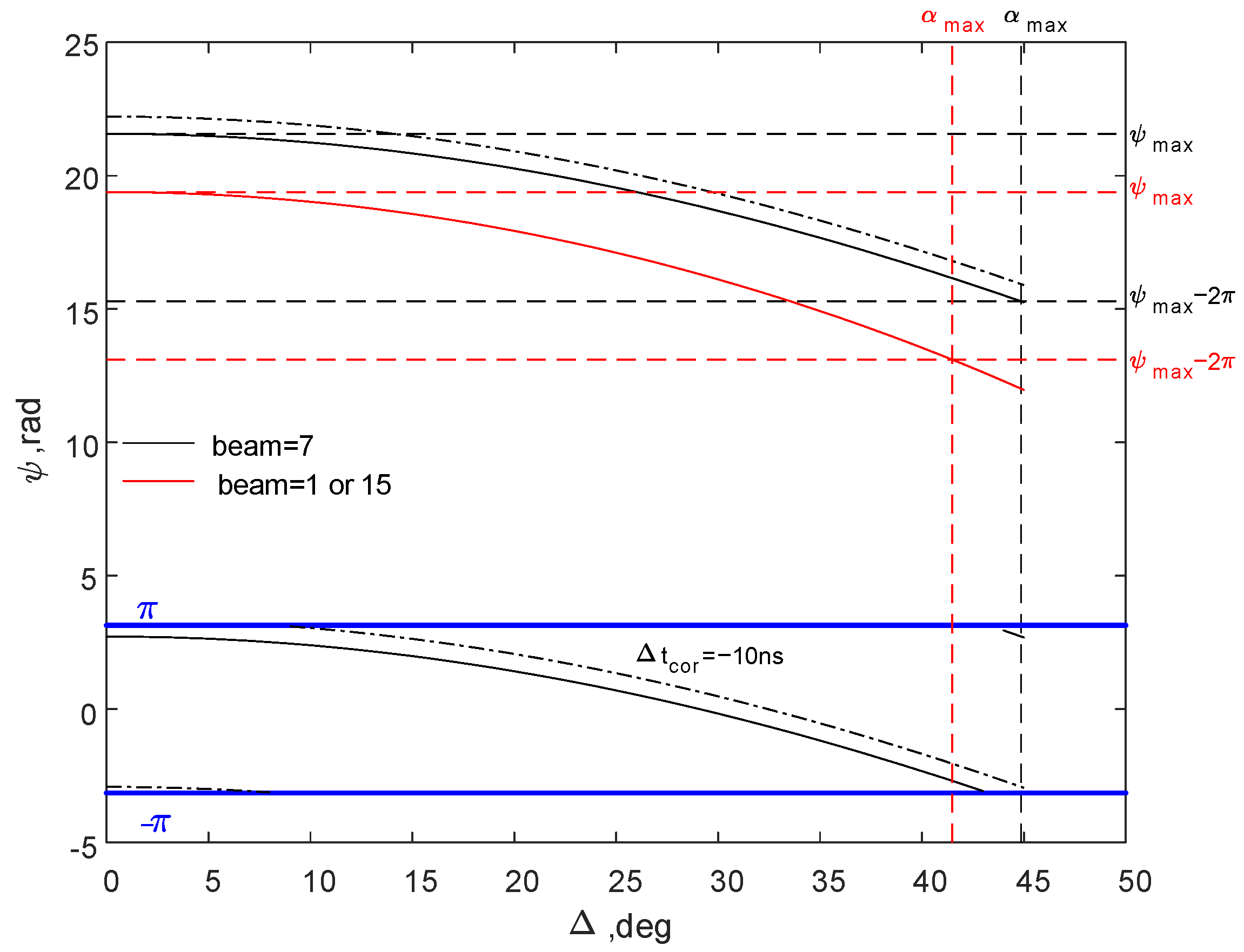
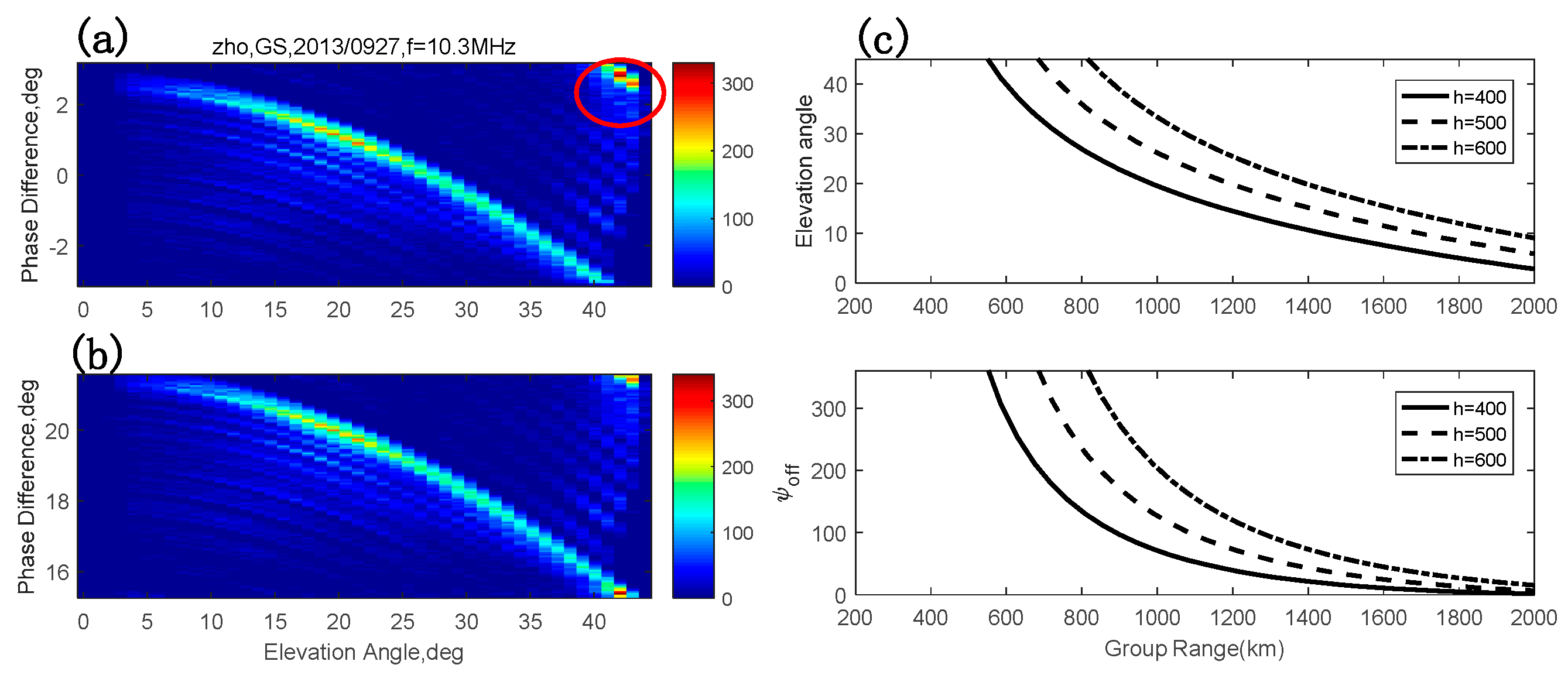
Then, we validate $\Delta t_{cor}$ with the phase offset at the specified virtual height. The phase difference in SuperDARN is preprocessed, it is within the phase range of $-\pi ~\pi$. However, the real phase difference should be considered with an ambiguous factor and located in ${\Psi }_{\max }-2\pi <{\Psi }_p\le {\Psi }_{\max }$. Figure 5a shows the relationship between the elevation angle and the phase difference of the radar data. There is a clear nonlinear relationship in the range of elevation of 0–40. A short line in the red circle deviates from the trend of the main curve, which is caused by different ambiguities at the time of the signal received by the radar. By adding ambiguity, the area in the red circle is consistent with the main distribution, as shown in Figure 5b. The azimuth angle of the echoes received on each beam is different, and this difference in the maximum phase causes a difference in the real phase interval. In the actual calibration process, the offset between the maximum phase and the phase ${\Psi }_{off}$ (phase offset) with the group range is selected as the calibrated data parameter.

There is a nonlinear function relationship between the elevation angle and phase difference from Equations (5) and (6). Therefore, we use the variation of ${\Psi }_{off}$ with the group range to determine $\Delta t_{cor}$. For echoes of low-angle propagation modes, the expected pattern of ${\Psi }_{off}$ is decreased with the increase in group range until the value approaches zero (Figure 5c). This is consistent with the study of Ponomarenko (2018) [1] using E region echoes. Furthermore, the phase offset ${\Psi }_{off}$ of the original data varying with the calibration factor $\Delta t_{cor}$ should approach the theoretical model curve at this virtual height, and the value of $\Delta t_{cor}$ is also close to that obtained in Figure 4. 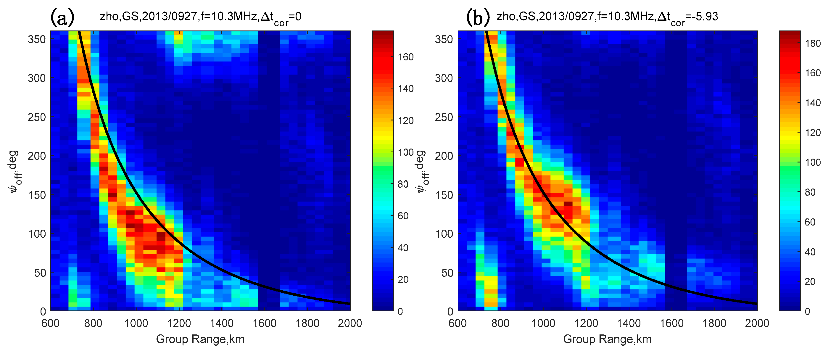Figure 6 shows the phase offset distribution of the ground echoes at the Zhongshan radar with a group range over 600 km. It can be seen that ${\Psi }_{off}$ decreased with the increase in group range, and the offset between all of the phase differences and the maximum phase was distributed in the range of $0<{\Psi }_{off}\le {360}^{°}$. The black solid line is the curve of ${\Psi }_{off}$ when the virtual height is 520 km, as shown in Figure 6. The calibration factor $\Delta t_{cor}$ of the radar is also determined according to the principle of the minimum RMSE. The ${\Psi }_{off}$ distribution in Figure 6a deviates significantly from the theoretical curve, especially for “discrete population” in the top of the group range at 1200–1400 km, with a phase deviation of approximately 22°. Figure 6b shows the distribution of the phase deviation changes with the group ranges with $\Delta t_{cor}\approx -5.93 \mathrm{ns}$. The center of the actual distribution is consistent with the theoretical curve.

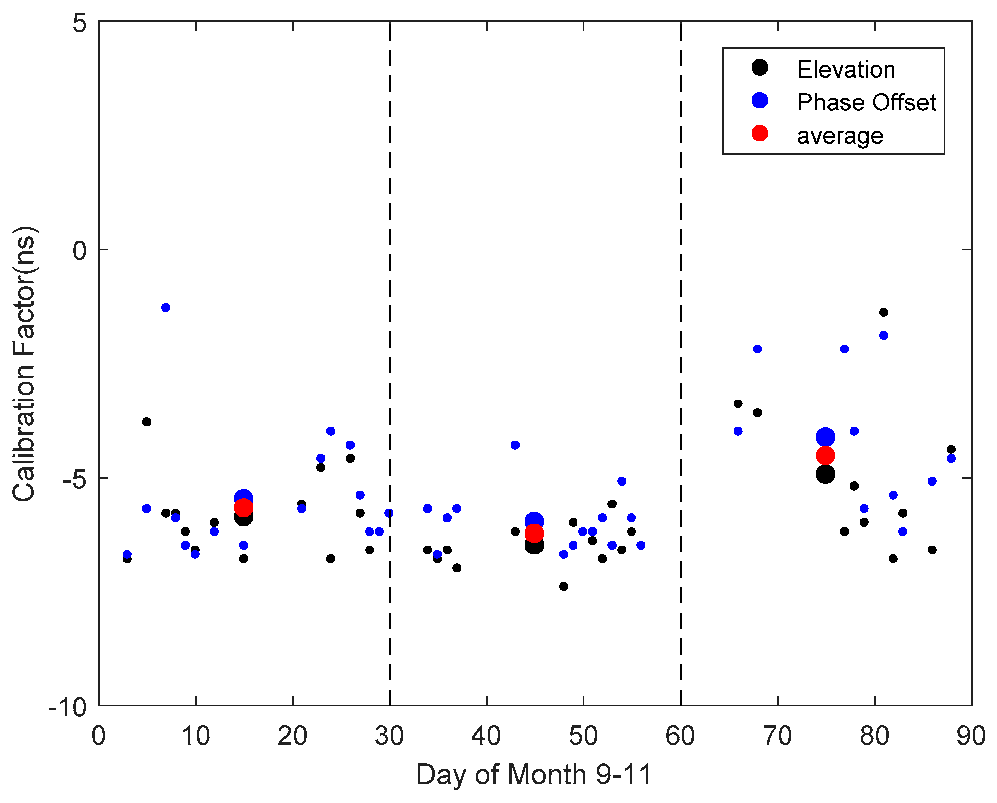
The data shown in Figure 6 show that the calibration factor $\Delta t_{cor}$ obtained by the phase offset verification is consistent with the elevation–virtual height model. Figure 7 shows the comparison of $\Delta t_{cor}$ determined by the two algorithms from September to November 2013. The black and blue dots are the daily calibration factors obtained by using the elevation angle and the phase offset, respectively. The black and blue solid circles correspond to the monthly mean calibration factors obtained by the daily calibration factors. There are some days with no data, which results in there being not enough ground echoes to calibrate. $\Delta t_{cor}$ is mostly concentrated between −5 and −7 ns, and the estimated values of the difference of two algorithms are generally less than 1 ns. The red solid circle is the mean value of the two methods, which is −5.68 ns, −6.24 ns, and −4.54 ns from September to November, respectively.

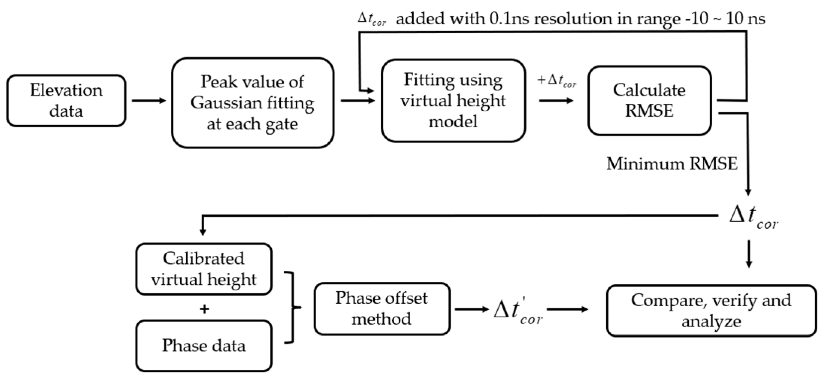
Given all of the information discussed above, the methodology for calibrating the elevation angle can be summarized, as shown in Figure 8.

4. Discussion

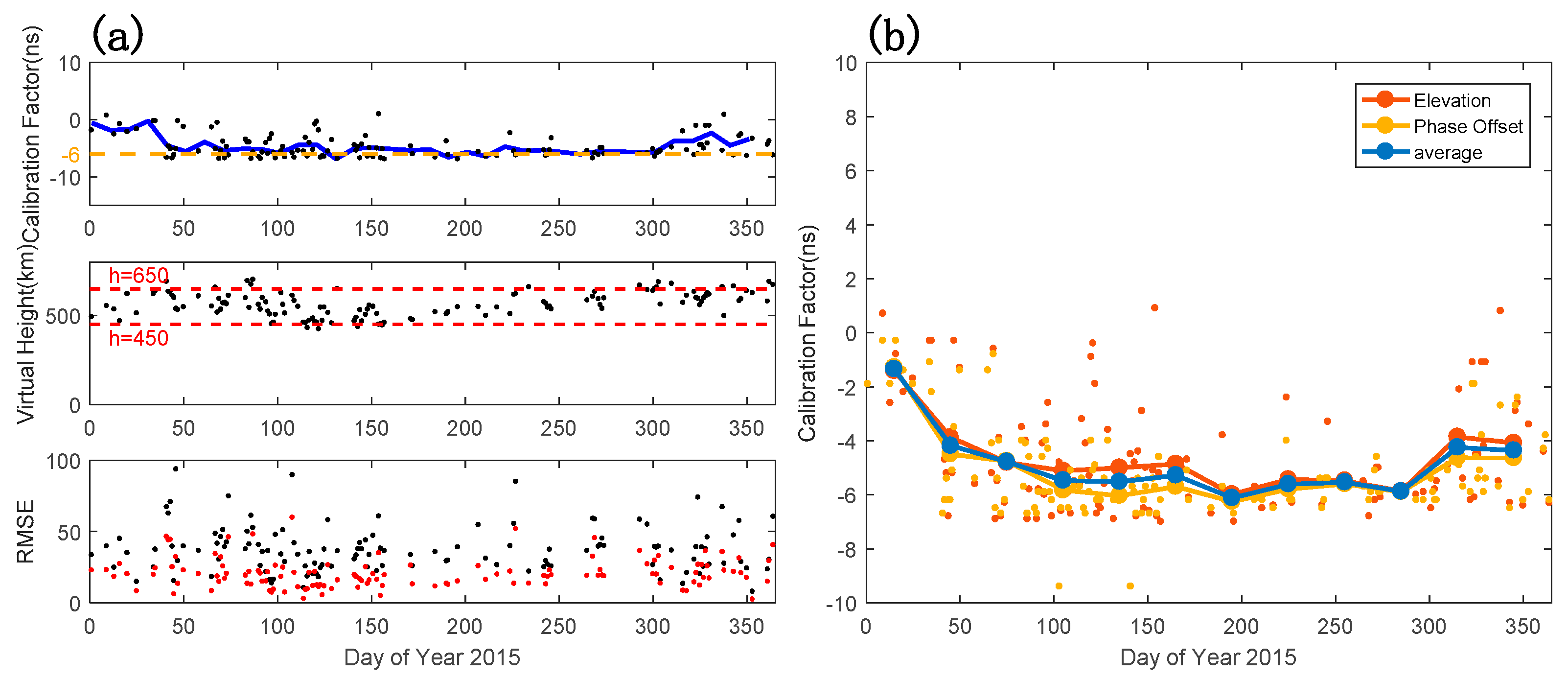
In this paper, the ground backscatter echoes of the Zhongshan radar from 2013 to 2015 are used to calculate the change in $\Delta t_{cor}$. The operating frequency of the Zhongshan radar is within 10.3 MHz ± 0.1 MHz, so the influence of the frequency for determining $\Delta t_{cor}$ is negligible. Figure 9 presents the results for 2015 at a daily resolution. The top of Figure 9a shows the variation in $\Delta t_{cor}$. The black dots represent the daily $\Delta t_{cor}$ calculated from the elevation data. As can be seen from the panel, the $\Delta t_{cor}$ distribution is relatively stable within a year, with a value concentrated around −6 ns, except for the first two months, which show values around -1 ns. The thick blue line shows a mean value of $\Delta t_{cor}$ at a temporal resolution of 10 days, this highlights the decrease in $\Delta t_{cor}$ around day 50 and slight fluctuations of $\Delta t_{cor}$ in the last two months. There will be a few deviation points, which may be due to the mixture of the echo type. The middle panel represents the change in the calibrated virtual height in one year. The red horizontal line indicates that the virtual height is 450 km and 650 km, and the calibrated virtual heights typically vary in this range. The fluctuation in virtual height shows no seasonal variation. This is because the distribution of the elevation angle is extended in different group ranges. The bottom of Figure 9a is the RMSE comparison of the virtual height before (black) and after (red) calibration. The RMSE before calibration is nearly double that of after calibration. For further verification, we estimate the average calibration factors using the elevation angle and phase offset. Figure 9b shows the change in $\Delta t_{cor}$ in 2015. The solid circle represents the values of the monthly average. The red and yellow line represent the $\Delta t_{cor}$ calculated according to the elevation information and the phase verification, respectively. The blue line represents the mean value. The monthly mean value of $\Delta t_{cor}$ shows a sharp decrease between January and February, while the monthly mean of the other months basically varies between −4 to −6 ns, which is consistent with the top of Figure 9a. The trend of the yellow line is similar to the red line, which verifies the reliability of $\Delta t_{cor}$.

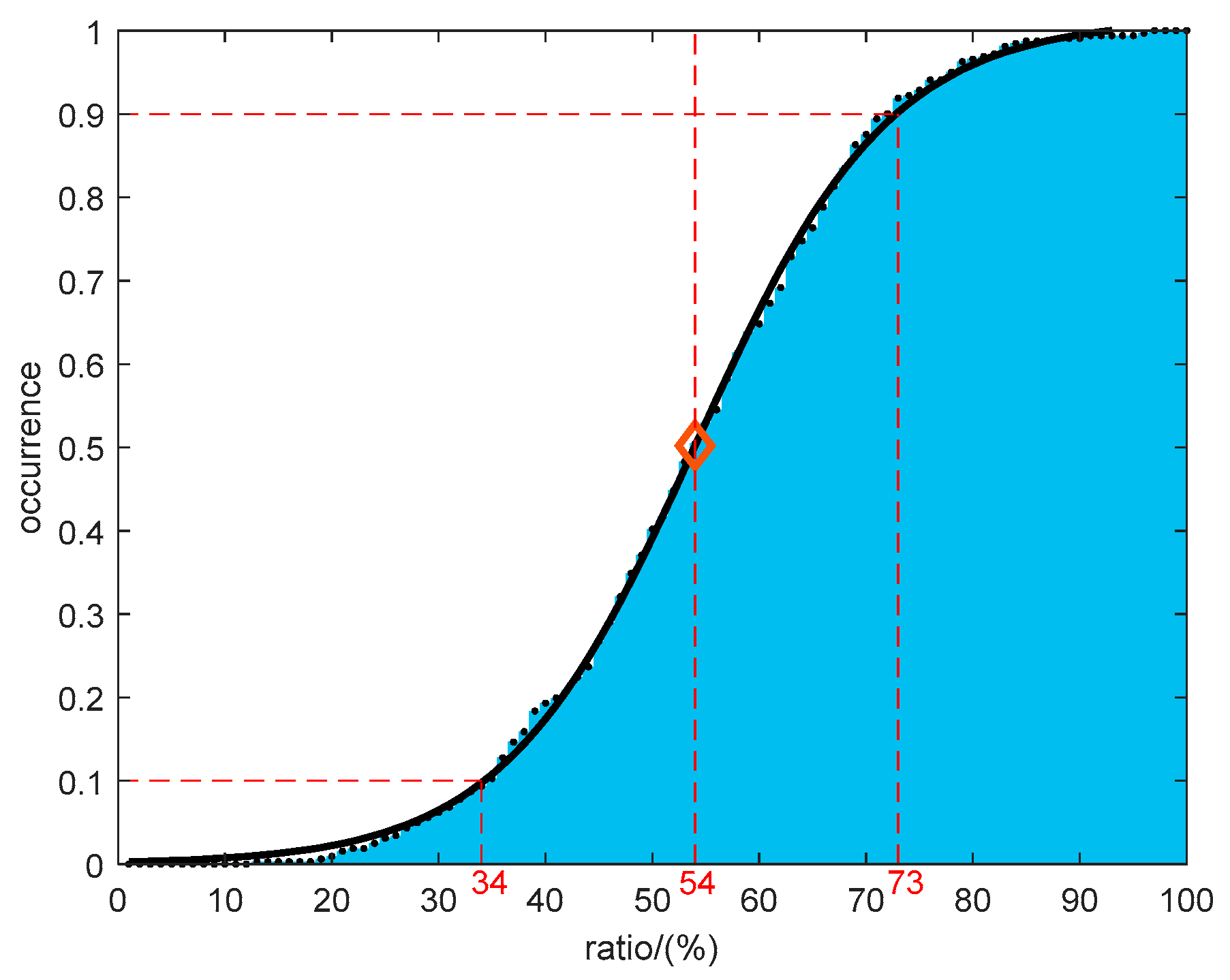
Figure 10 shows the statistical distribution histogram of RMSE before and after calibration for 2013–2015. We calculated the distribution of the RMSE ratio before and after calibration, presenting a probability histogram for each ratio, and used the Logistic algorithm to fit. The results show that the ratio is concentrated between 34% and 73%. The maximum slope represents the peak value of the ratio occurrence. The RMSE of the group range–elevation distribution is mostly reduced to within 54%.

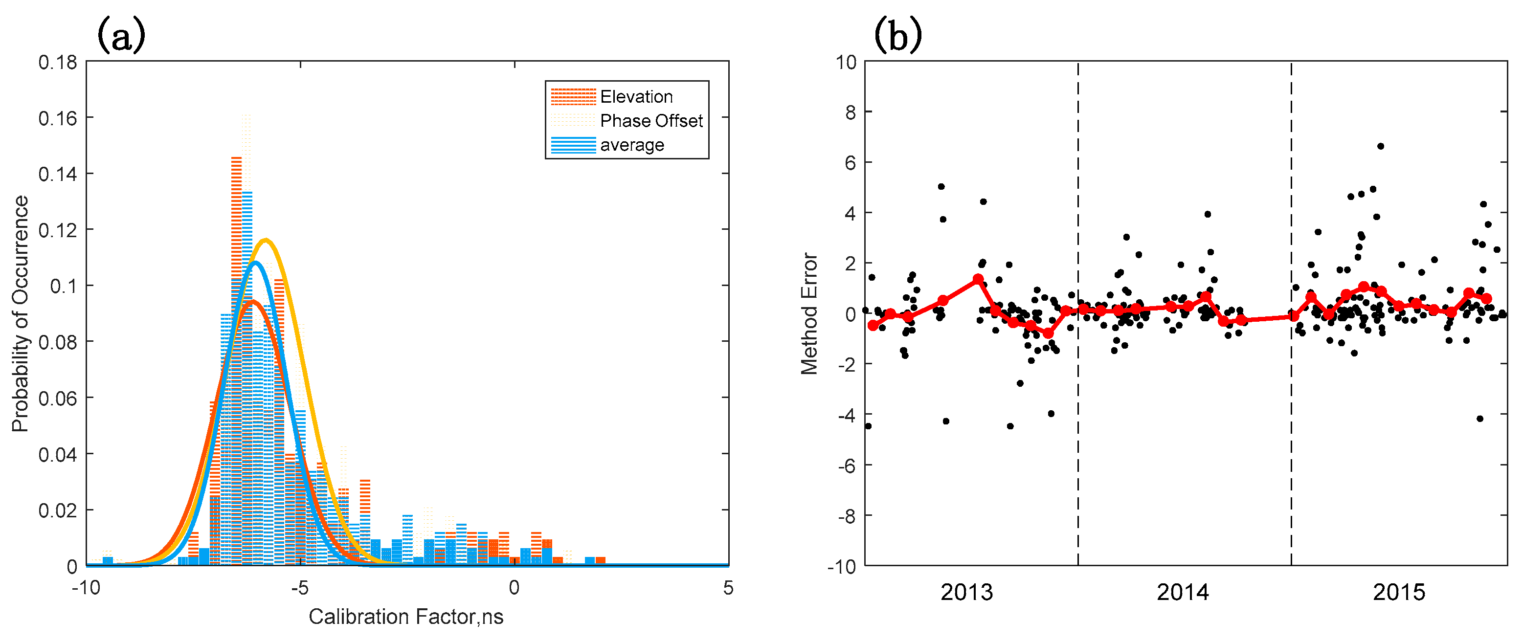
Figure 11a describes the probability distribution of $\Delta t_{cor}$ from 2013 to 2015. The red and yellow histograms represent $\Delta t_{cor}$ estimated by the elevation and phase verification, respectively, most of the values appear between −5 ns and −7 ns, and the two distributions are consistent. The blue histogram represents the change in the mean value. The values of $\Delta t_{cor}$ corresponding to the Gaussian fitting peaks are −6.1 ns (red), −5.8 ns (yellow), and -6.06 ns (blue). The results reflect that the $\Delta t_{cor}$ of the Zhongshan radar is about −6 ns in most conditions. The change in $\Delta t_{cor}$ error calculated between the two algorithms over three years is shown in Figure 11b. The black dot is the daily $\Delta t_{cor}$ difference change calculated according to the two algorithms, and the data without ground backscatter characteristic curves should be excluded. The estimated $\Delta t_{cor}$ by RMSE and ${\Psi }_{off}$ within three years is maintained within 2 ns, and most of them are less than 1 ns. The thick red line is the monthly average $\Delta t_{cor}$ calculated according to the daily value, which reduces the random noise in the diurnal variation to a certain extent. Monthly statistical results show that the error of the two algorithms is basically less than 1 ns, which proves that the $\Delta t_{cor}$ estimated by RMSE has a good reliability.

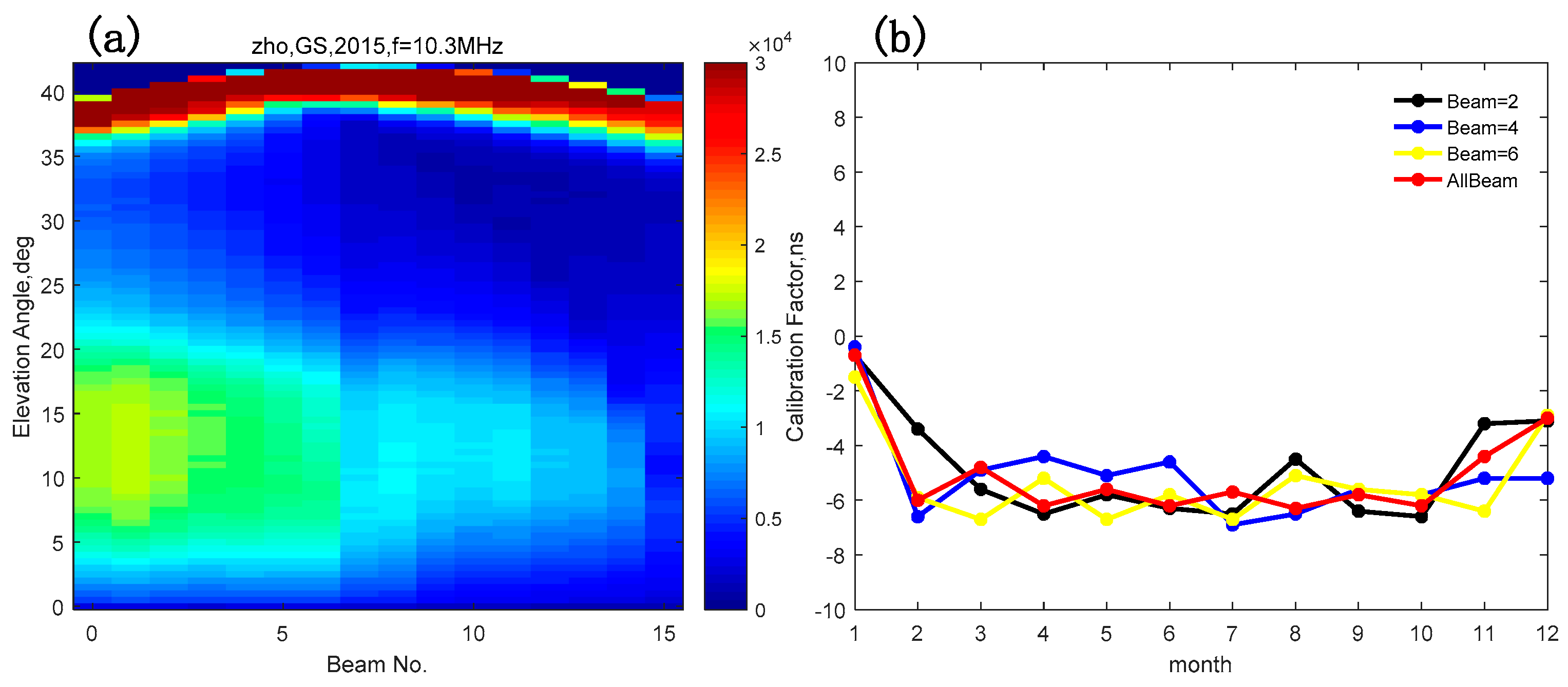
When the Zhongshan radar receives the echoes returned from all directions, it will be equally divided into 16 fan-shaped echo receiving areas in the sweep mode. Figure 12 shows the elevation distribution measured by each beam at the Zhongshan radar for one month. From the Figure 12a, there is a high elevation angle curve band, which is the result of the aliased elevation measurements [14]. For the Zhongshan radar, the number of echoes varies with the beams. Overall, the most elevation angle information is from the beams with small numbers, with an obvious broadband from 5° to 20°, this is due to the coverage for different beams. Although the method discussed above uses data for all beams, we also considered that the values of the calibration factors may change with the beams. Figure 12b shows the change in $\Delta t_{cor}$ over one year based on monthly statistics for beam 2, 4, 6, and all, respectively. The change in $\Delta t_{cor}$ is smoother than that of the diurnal variation (not shown). The value of $\Delta t_{cor}$ shows the same variation through the year of the diurnal variation, and its value fluctuates around −6 ns and does not change with the beam significantly, except in January, which is consistent with Figure 8b.

5. Conclusions

Considering the time delay caused by the path difference between the signal and two antenna arrays in the SuperDARN radar, this paper uses ground backscatter to calibrate the elevation angle data. Considering the minimum RMSE of the virtual height at different group ranges before and after calibration and using the phase offset with the group range under the specific virtual height to comprehensively analyze and determine the optimal value of $\Delta t_{cor}$, the results show that the estimated and verified $\Delta t_{cor}$ are relatively consistent. Applied in the ground backscatter of the Zhongshan radar for several years, the value of $\Delta t_{cor}$ is maintained in the range of −5~−7 ns, which indicates that this method is not constrained by s time scale, without considering the changes caused by external factors.

According to the comparison above, this paper draws the following conclusions:

(1)

The peak point of the group range–elevation angle distribution under each range gate is used as the input, and the virtual height is fitted. The RMSE of the virtual height before and after calibration is calculated and compared. The high accuracy of $\Delta t_{cor}$ is implemented by a step of 0.1 ns. The value of $\Delta t_{cor}$ is taken when the RMSE is at minimum, and the calibrated virtual height is obtained. The phase deviation drawn by the original phase data is compared with that of the virtual height to verify the reliability of $\Delta t_{cor}$. The results show that $\Delta t_{cor}$ is relatively consistent.

(2)

Nearly all of the calibrated RMSE decreased to 73% of the original. Most of the RMSE ratio can be reduced to 54%, indicating that the deviation between the observed value and the true value was significantly improved after adding $\Delta t_{cor}$.

(3)

The possible influence of beams on the calibration process are presented. The theoretical analysis shows that the influence of the beam on the conclusion is neglected, but its specific difference should be analyzed in detail in follow-up studies.

References

1. Ponomarenko, P.; Maurice, J.S.; McWilliams, K. Calibrating HF radar elevation angle measurements using E layer backscatter echoes. Radio Sci. 2018, 53, 1438–1449. [Google Scholar] [CrossRef]
2. McDonald, A.J.; Whittington, J.; Larquier, S.; Custovic, E.; Kane, T.A.; Devlin, J.C. Elevation angle-of-arrival determination for a standard and a modified SuperDARN HF radar layout. Radio Sci. 2013, 48, 709–721. [Google Scholar] [CrossRef]
3. Ribeiro, A.J.; Ruohoniemi, J.M.; Baker, J.B.H.; Clausen, L.B.N.; de Larquier, S.; Greenwald, R.A. A new approach for identifying ionospheric backscatter in midlatitude SuperDARN HF radar observations. Radio Sci. 2011, 46, 1–11. [Google Scholar] [CrossRef]
4. Shepherd, S. Elevation angle determination for SuperDARN HF radar layouts. Radio Sci. 2017, 52, 938–950. [Google Scholar] [CrossRef]
5. Deng, T.Y.; Liu, E.X.; Xu, C. SuperDARN polar ionospheric convection potential model based on deep learning. Chin. J. Geophys. 2022, 65, 819–829. [Google Scholar] [CrossRef]
6. Thayyil, J.P.; McCaffrey, A.M.; Wang, Y.; Themens, D.R.; Watson, C.; Reid, B.; Zhang, Q.H.; Xing, Z.Y. Global positioning system (GPS) scintillation associated with a polar cap patch. Remote Sens. 2021, 13, 1915. [Google Scholar] [CrossRef]
7. Chisham, G.; Freeman, M.P. A reassessment of SuperDARN meteor echoes from the upper mesosphere and lower thermosphere. J. Atmos. Sol. -Terr. Phys. 2013, 102, 207–221. [Google Scholar] [CrossRef] [Green Version]
8. Greenwald, R.A.; Frissell, N.; Larquier, S. The importance of elevation angle measurements in HF radar investigations of the ionosphere. Radio Sci. 2017, 52, 305–320. [Google Scholar] [CrossRef]
9. Chisham, G. Calibrating SuperDARN interferometers using meteor backscatter. Radio Sci. 2018, 53, 761–774. [Google Scholar] [CrossRef]
10. Ponomarenko, P.; Nishitani, N.; Oinats, A.V.; Tsuya, T.; St-Maurice, J.P. Application of ground scatter returns for calibration of HF interferometry data. Earth Planets Space 2015, 67, 7003. [Google Scholar] [CrossRef]
11. Coluccia, A.; Fascista, A.; Ricci, G. Design of Customized Adaptive Radar Detectors in the CFAR Feature Plane. arXiv 2022, arXiv:2203.12565. preprint. [Google Scholar] [CrossRef]
12. Ma, W.J.; Tu, G.Y.; Deng, Z.M.; Lu, X.F.; Ye, Y.S.; Li, Y.H. A novel wideband radar detector via Wiener filter. Electron. Lett. 2022, 58, 505–507. [Google Scholar] [CrossRef]
13. Goh, C.; Devlin, J.C.; Deng, D.; McDonald, A.; Kamarudin, M.R. Uncorrelated weighted median filtering for noise removal in superdarn. In Proceedings of the 2014 IEEE 17th International Conference on Computational Science and Engineering, Chengdu, China , 19–21 December 2014; pp. 981–988. [Google Scholar] [CrossRef]
14. Chisham, G.; Burrell, A.G.; Marchaudon, A.; Shepherd, S.G.; Thomas, E.G.; Ponomarenko, P. Comparison of interferometer calibration techniques for improved SuperDARN elevation angles. Polar Sci. 2021, 28, 100638. [Google Scholar] [CrossRef]
15. Burrell, A.G.; Yeoman, T.K.; Milan, S.E.; Lester, M. Phase calibration of interferometer arrays at high-frequency radars. Radio Sci. 2016, 51, 1445–1456. [Google Scholar] [CrossRef] [Green Version]
16. Chisham, G.; Yeoman, T.K.; Sofko, G. Mapping ionospheric backscatter measured by the SuperDARN HF radars–Part 1: A new empirical virtual height model. Ann. Geophys. 2008, 26, 823–841. [Google Scholar] [CrossRef] [Green Version]
17. Yeoman, T.K.; Chisham, G.; Baddeley, L.; Dhillon, R.; Karhunen, T.; Robinson, T.; Senior, A.; Wright, D. Mapping ionospheric backscatter measured by the SuperDARN HF radars–Part 2: Assessing SuperDARN virtual height models. Ann. Geophys. 2008, 26, 843–852. [Google Scholar] [CrossRef] [Green Version]
18. Li, G.M.; Yan, J.Y.; Lan, A.L. An Improved Meteor Echo Recognition Algorithm for SuperDARN HF Radar. Electronics 2021, 10, 1971. [Google Scholar] [CrossRef]
19. Liu, J.J.; Hu, H.Q.; Chen, X.C. A dataset from the Zhongshan HF coherent scatter radar in Antarctica (2012). China Sci. Data 2021, 6. [Google Scholar] [CrossRef]
20. Gillies, R.G.; Hussey, G.C.; Sofko, G.J.; McWilliams, K.A.; Fiori, R.A.D.; Ponomarenko, P.; St-Maurice, J.P. Improvement of SuperDARN velocity measurements by estimating the index of refraction in the scattering region using interferometry. J. Geophys. Res. Space Phys. 2009, 114, A07305. [Google Scholar] [CrossRef]
21. Hall, G.E.; MacDougall, J.W.; Moorcroft, D.R.; St-Maurice, J.P.; Manson, A.H.; Meek, C.E. Super dual auroral radar network observations of meteor echoes. J. Geophys. Res. Space Phys. 1997, 102, 14603–14614. [Google Scholar] [CrossRef]
22. André, D.; Sofko, G.J.; Baker, K.; MacDougall, J. SuperDARN interferometry: Meteor echoes and electron densities from groundscatter. J. Geophys. Res. Space Phys. 1998, 103, 7003–7015. [Google Scholar] [CrossRef]
23. Liu, E.X.; Hu, H.Q.; Hosokawa, K.; Liu, R.Y.; Wu, Z.S.; Xing, Z.Y. First observations of polar mesosphere summer echoes by SuperDARN Zhongshan radar. J. Atmos. Sol. -Terr. Phys. 2013, 104, 39–44. [Google Scholar] [CrossRef]
24. Ponomarenko, P.V.; Koustov, A.V.; St-Maurice, J.P.; Wiid, J. Monitoring the F-region peak electron density using HF backscatter interferometry. Geophys. Res. Lett. 2011, 38, L21102. [Google Scholar] [CrossRef]
25. Berngardt, O.I.; Fedorov, R.R.; Ponomarenko, P.; Grkovich, K.V. Interferometric calibration and the first elevation observations at EKB ISTP SB RAS radar at 10–12 MHz. Polar Sci. 2021, 28, 100628. [Google Scholar] [CrossRef]
26. Burrell, A.G.; Milan, S.E.; Perry, G.W.; Yeoman, T.K.; Lester, M. Automatically determining the origin direction and propagation mode of high-frequency radar backscatter. Radio Sci. 2015, 50, 1225–1245. [Google Scholar] [CrossRef]
Figure 1. (a) The positional relationship diagram of main array and interferometer array of SuperDARN; (b) field of views (FOVs) of the Zhongshan high frequency radar (ZHO).
Electronics 11 04236 g001
Figure 2. The relationship between the elevation angle and the phase difference for d = 100 m, f = 10.3 MHz (Zhongshan radar), the black line represents the boresight direction, and the red line represents the edge of the field of view. The solid blue horizontal line indicates that the phase difference is limited between π and π measured by the radar when the ambiguity factor is not considered. The black and red horizontal dashed line represents the actual phase range Ψ max ~ Ψ max 2 π , and the black and red vertical dashed line represents the maximum elevation angle α max .
Electronics 11 04236 g002
Figure 3. The virtual height distribution of ground backscatter echoes for range gate 24 (1215–1260 km) at the Zhongshan radar in September 2013. The black line represents the actual virtual height calculated by the elevation angle and group range, and the red line represents the result of fitting with a Gaussian function.
Electronics 11 04236 g003
Figure 4. The distribution of the elevation angle (top) and virtual height (bottom) of all beams of the ground backscatter echoes from the Zhongshan radar on 27 September 2013, where the radar frequency is 10.3 MHz. (a) The original (uncalibrated) data; (b) data calibrated with Δ t c o r = 6 n s . Black dots and lines at the top correspond to peak elevation of each gate and fitting curve. Error bars at the bottom show the actual and fitting deviations.
Electronics 11 04236 g004
Figure 5. The same data as Figure 4, (a) the measured data and (b) the elevation–phase difference change with ambiguity factor added. (c) theoretical group range–elevation and group range–phase offset trends at h = 400, 500, and 600 km. The red circle in panel (a) shows ambiguity in the phase difference measurement.
Electronics 11 04236 g005
Figure 6. Number of echoes between the phase deviation and the group range from Zhongshan radar on 27 September 2013. The solid black line represents the theoretical relationship between the phase deviation and the group range when the virtual height is 520 km. (a) the original (uncalibrated) data; (b) data calibrated with Δ t c o r = 5.93   ns .
Electronics 11 04236 g006
Figure 7. Daily and monthly average calibration factor for both methods.
Electronics 11 04236 g007
Figure 8. Flowchart of the main step of the proposed method.
Electronics 11 04236 g008
Figure 9. (a) The estimated calibration factor (top), mean virtual height (middle), and RMSE comparison before and after calibration (bottom), from the Zhongshan radar in 2015. The yellow dotted line on the top panel represents a calibration factor of −6 ns and the blue line represents the mean value from 10 days. The red dotted line in the middle panel represents a virtual height of 450 km and 650 km. (b) Statistical distribution of the calibration factors for the two methods in 2015, elevation angle (red), phase offset (yellow), and average of two (blue). Dots represent daily distributions, filled circles represent monthly distributions, and line graphs represent monthly averages calculated from the daily estimates.
Electronics 11 04236 g009
Figure 10. RMSE ratio distribution histogram before and after calibration for 2013–2015. Black dots show the probability of RMSE ratio below this ratio, and black line represents logistic fit results. The vertical dashed line with red lozenge outlines the maximum slope of fitting.
Electronics 11 04236 g010
Figure 11. (a) The elevation angle (Red), the measured phase offset (yellow), and the average of two algorithms (blue) used to obtain the statistical distribution of the calibration factor. Curve represents the result of Gaussian fitting. (b) Two algorithm calibration factor error, black and red dots represent the daily and monthly average changes, respectively.
Electronics 11 04236 g011
Figure 12. (a) The histograms of the beam number and elevation angle distributions observed by the Zhongshan radar. (b) Monthly variation of different beam calibration factors in 2015.
Electronics 11 04236 g012
Publisher’s Note: MDPI stays neutral with regard to jurisdictional claims in published maps and institutional affiliations.