Comparative Estimation of Electrical Characteristics of a Photovoltaic Module Using Regression and Artificial Neural Network Models

Abstract

Accurate modeling of photovoltaic (PV) modules under outdoor conditions is essential to facilitate the optimal design and assessment of PV systems. As an alternative model to the translation equations based on regression methods, various data-driven models have been adopted to estimate the current–voltage (I–V) characteristics of a photovoltaic module under varying operation conditions. In this paper, artificial neural network (ANN) models are compared with the regression models for five parameters of a single diode solar cell. In the configuration of the proposed PV models, the five parameters are predicted by regression and neural network models, and these parameters are put into an explicit expression such as the Lambert W function. The multivariate regression parameters are determined by using the least square method (LSM). The ANN model is constructed by using a four-layer, feed-forward neural network, in which the inputs are temperature and solar irradiance, and the outputs are the five parameters. By training an experimental dataset, the ANN model is built and utilized to predict the five parameters by reading the temperature and solar irradiance. The performance of the regression and ANN models is evaluated by using root mean squared error (RMSE) and mean absolute percentage error (MAPE). A comparative study of the regression and ANN models shows that the performance of the ANN models is better than the regression models.

1. Introduction

The output power of photovoltaic (PV) systems is strongly affected under arbitrary operating conditions such as temperature and solar irradiance of PV modules [1,2]. However, highly predictive and efficient models across different temperatures and irradiances have not been established [3,4,5,6]. In addition, their nonlinear characteristics make highly predictive modeling even more difficult [7,8,9,10,11,12,13]. The single-diode model (SDM) with five parameters is widely utilized to reproduce the current–voltage (I–V) characteristics [5,6,7,8]. Owing to the inherent implicit expression for the electrical equivalent circuit of the SDM, analytical and explicit I–V models have been proposed to calculate the I–V relationship [1,14,15,16]. The explicit I–V model based on the Lambert W function is simple and efficient, while the implicit model requires more computational time [14,15,16]. Although optimization methods have been proposed to obtain the five parameters at the standard test condition (STC), significant extraction efforts are required to consider the dependence of unknown parameters on temperature and solar irradiance [3,4,5,6,7,8,17,18,19,20,21]. For arbitrary operating conditions, the performance of the parameter translation model is greatly limited by the chosen translation equation and correction factors [13,17,18,19,20,21]. In order to construct a complete PV model for climatic conditions, the translational formula should be further modified [17,19] and new parameters may need to be taken into account [18,20,21]. Moreover, the accuracy of the translational formula varies significantly at low irradiance levels [3,4,5]. However, artificial neural network (ANN) models provide parameter identification, I–V prediction with higher accuracy directly from the measured data [22,23], and fault detection and diagnosis for photovoltaic systems [24,25,26]. To accurately estimate the performance of PV modules under varying operating conditions, it is necessary to establish a data-driven model for the five parameters with change in irradiance and temperature [27,28,29,30,31,32,33,34,35,36,37]. In recent years, improved ANN models have been proposed by adding more variables [38] and utilizing the efficient training schemes and processing of neural networks [39,40,41,42]. This paper compares the performance of regression and ANN models for the five parameters in predicting the I–V relationship of a PV module based on an explicit expression. The results show that the ANN model provides better performance than the regression model. The novelty of the proposed approach lies primarily in the successful integration of comparative models into an analytical and explicit Lambert W function, in contrast with the previous practice for the electrical equivalent circuits. (1) In this new framework, temperature and solar irradiance serve as inputs to establish the regression and ANN models for I–V prediction under arbitrary operating conditions. (2) An advanced ANN model for the five parameters is developed by determining an optimum ANN architecture to improve the estimation of the model. The ANN model developed can provide an efficient method with higher accuracy in predicting I–V characteristics, compared to the regression model.

In this work, the modeling process begins in Section 2 with the theoretical formulation of an explicit I–V model and translation equations for the five parameters. Section 3 describes the regression and ANN models, followed in Section 4 by a comparative validation of both the models against the experimental data for a PV module. In Section 5, the main conclusions are drawn.

2. Theoretical Models

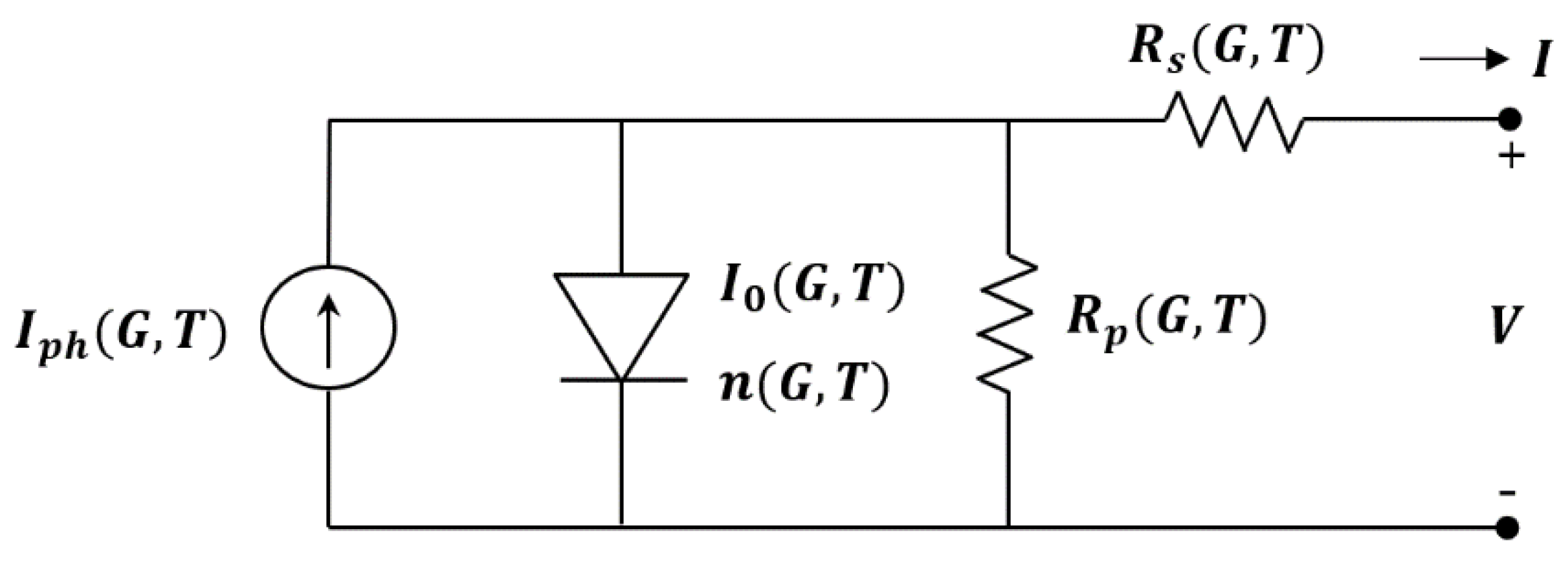
2.1. Explicit and Analytical I–V Model

The PV-equivalent circuit of a single diode with two resistors is shown in Figure 1. The I–V relationship of a PV module can be expressed with a single diode as [1,2,5,6,7,8]:

$$I=I_{ph}-I_0\left[\exp \left(\frac{V+I{R}_s}{n{V}_t}\right)-1\right]-\frac{V+I{R}_s}{R_p}$$

(1)

where $I_{ph}$ is the photogenerated current, $I_0$ is the diode reverse saturation current, $n$ is the ideality factor, and $R_s$ and $R_p$ is the series and parallel resistance, respectively. The thermal voltage is given by $V_t=N_s{k}_{b}T/q$, where $N_s$ is the number of series-connected cells, $k_b$ is the Boltzmann constant, and $T$ is the temperature. The explicit solution of the PV module transcendent Equation (1) is given as a function of the Lambert W function [1,14,15,16]:

$$I=\frac{R_p\left(I_{ph}+I_0\right)-V}{R_s+R_p}-\frac{n{V}_t}{R_s}W\left(\alpha \left(V\right)\right)$$

(2)

$$\alpha \left(V\right)=\frac{R_s{R}_p{I}_0}{n{V}_t\left(R_s+R_p\right)}{e}^{\frac{R_p\left(R_s{I}_{ph}+R_s{I}_0+V\right)}{n{V}_t\left(R_s+R_p\right)}}$$

(3)

2.2. Five Parameters as a Function of Temperature and Solar Irradiance

Environmental conditions such as temperature (T) and solar irradiance (G) have strong effects on the I–V characteristics of the PV module. In order to extract accurate estimates of the model parameters under arbitrary T and G, mathematical expressions for the five parameters are reformulated by using the advantage of the previous formula [1,2,5,6,7,8]. The I–V curve translation for desired solar irradiance and temperature (G, T) from STC ($G_0$,$T_0$) is obtained by using the short circuit current ($I_{sc})$ and the open circuit voltage ($V_{oc}$). Assuming the condition $I_{sc}\approx I_{ph}$, $I_{sc}\left(G,T\right)$ and $V_{oc}\left(G,T\right)$ are determined as [1,2,5,6,7,8]:

$$I_{sc}\left(G,T\right)\approx I_{ph}\left(G,T\right)=\left(\frac{G}{G_0}\right)\left[I_{ph0}+{\alpha }_i\left(T-T_0\right)\right]$$

(4)

$$V_{oc}\left(G,T\right)=V_{oc0}\left[1+{\alpha }_v\left(T-T_0\right)+{\beta }_v{V}_t\ln \left(\frac{G}{G_0}\right)\right]$$

(5)

where $I_{ph0}$ and $V_{oc0}$ are the photogenerated current and open circuit voltage at standard test conditions, respectively; ${\alpha }_i$ and ${\alpha }_v$ are temperature coefficients and ${\beta }_v$ is an irradiance coefficient. From the relationship $n=n_0\left(V_{oc}/V_{oc0}\right)$ and $R_{s,p}=R_{s0,p0}\left(V_{oc}/V_{oc0}\right)\left(I_{sc0}/I_{sc}\right)$, the values of the translated parameters $n\left(G,T\right)$, $R_s\left(G,T\right)$, and $R_p\left(G,T\right)$ are calculated as follows [1,2,7]:

$$n\left(G,T\right)=n_0\left[1+{\alpha }_n\left(T-T_0\right)+{\beta }_n{V}_t\ln \left(\frac{G}{G_0}\right)\right]$$

(6)

$$R_s\left(G,T\right)=R_{s0}\frac{1+{\alpha }_{R_s}\left(T-T_0\right)+{\beta }_{R_s}{V}_t\ln \left(\frac{G}{G_0}\right)}{\left(\frac{G}{G_0}\right)\left[1+{\alpha }_{R_s}^{*}\left(T-T_0\right)\right]}$$

(7)

$$R_p\left(G,T\right)=R_{p0}\frac{1+{\alpha }_{R_p}\left(T-T_0\right)+{\beta }_{R_p}{V}_t\ln \left(\frac{G}{G_0}\right)}{\left(\frac{G}{G_0}\right)\left[1+{\alpha }_{R_p}^{*}\left(T-T_0\right)\right]}$$

(8)

where $n_0$, $R_{s0}$, and $R_{p0}$ are the ideality factor, series resistance, and parallel resistance at standard test conditions, respectively; ${\alpha }_n$, ${\alpha }_{R_s}$, ${\alpha }_{R_s}^{*}$, ${\alpha }_{R_p}$, and ${\alpha }_{R_p}^{*}$ are temperature coefficients and ${\beta }_n, {\beta }_{R_s}$, and ${\beta }_{R_p}$ are irradiance coefficients. By setting $I=0$ in (1), the translation expression for the reverse saturation current $I_0\left(G,T\right)$ as a function of $I_{ph}\left(G,T\right)$, $V_{oc}\left(G,T\right)$, $n\left(G,T\right)$, and $R_{s,p}\left(G,T\right)$ is obtained as [1,2,7]:

$$I_0\left(G,T\right)=\frac{I_{ph}\left(G,T\right)-\frac{V_{oc}\left(G,T\right)}{R_p\left(G,T\right)}}{\exp \left(\frac{V_{oc}\left(G,T\right)}{n\left(G,T\right) V_t}\right)-1}$$

(9)

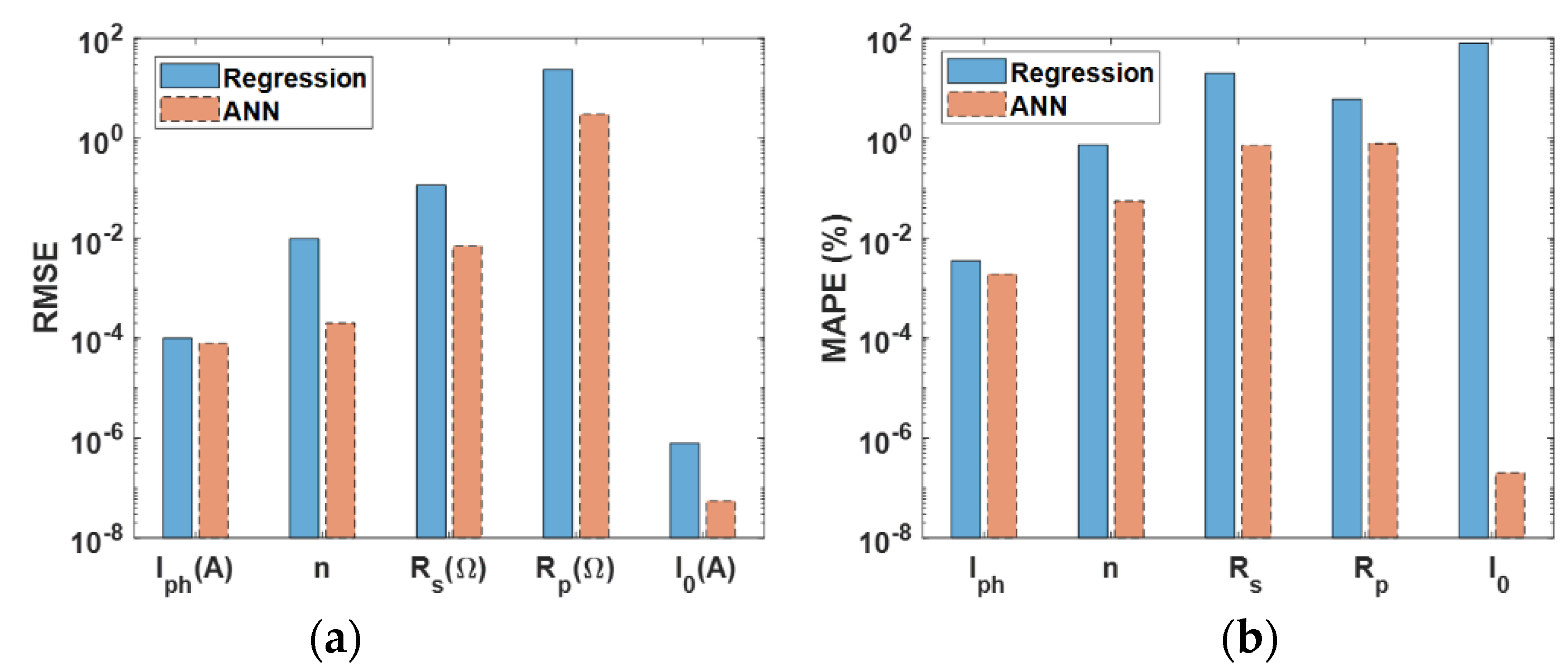
3. Parameter Identification Approaches

3.1. Multiple Regression

The multivariate regression analysis is employed to model the statistical relationship between inputs ($G$,$T$) and outputs ($I_{ph}$,$n$,$R_s$,$R_p$,$I_0$). The parametric regression equation for a linear or nonlinear function $f$ is expressed as [43,44,45]:

$$y=f\left(X_1,\dots ,X_n;{\theta }_1,\dots ,{\theta }_m\right)+\epsilon$$

(10)

where $y$ is an $n\times 1$ vector of dependent variable, $X_1,\dots ,X_n$ are an $n\times m$ matrix of independent variables, ${\theta }_1,\dots ,{\theta }_m$ are an $m\times 1$ vector of regression parameters, and $\epsilon$ is an $n\times 1$ vector of random error. The regression parameters ${\theta }_1,\dots ,{\theta }_m$ are usually determined using the least square method (LSM) to minimize $\sum _{i=1}^k{\left(y_i-f\left(X_{1i},\dots ,X_{ni};{\theta }_1,\dots ,{\theta }_m\right)\right)}^2$ with different sample points k. Based on the estimated regression parameters, the optimum regression model is chosen for prediction.

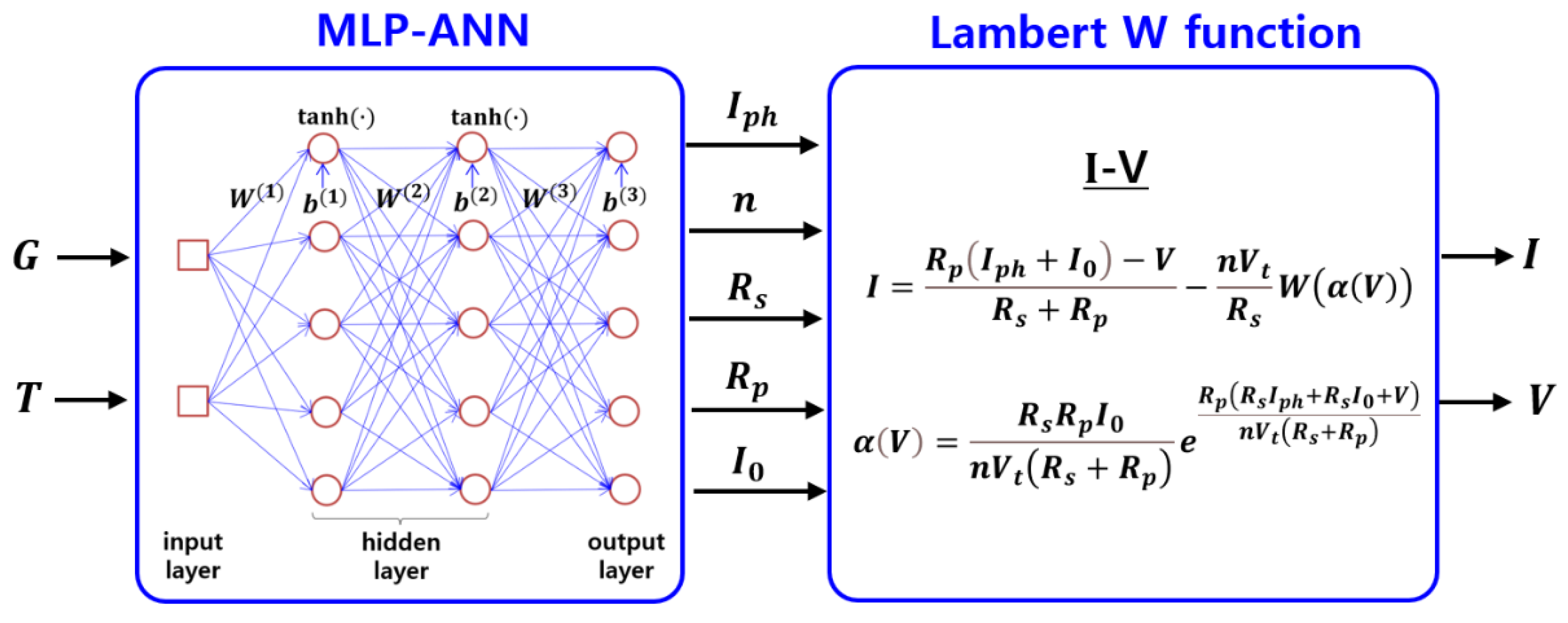
3.2. Artificial Neural Network (ANN)

The artificial neural network is specified in modeling complex systems, especially nonlinear or random variable systems. The multilayer perceptron (MLP), known as the fully connected feed-forward network for supervised learning, is the most common and successful for modeling nonlinear systems [22,23,31]. The MLP network configuration has an input layer, two hidden layers, and an output layer. The input layer consists of two neurons ($G$,$T$), and the output layer contains five neurons ($I_{ph}$,$n$,$R_s$,$R_p$,$I_0$). Every neuron in one layer is fully connected to every neuron in the next layer. By using the activation function of a hyperbolic tangent sigmoid function for N neurons, the output $h_i^{\left(k\right)}$ of the ith neuron in the $k$th hidden layer is computed as follows [22,23]:

$$h_i^{\left(1\right)}=\tanh \left({\displaystyle \sum }_{j=1}^2{w}_{ij}^{\left(1\right)}{x}_j+b_i^{\left(1\right)}\right)$$

(11)

$$h_i^{\left(2\right)}=\tanh \left({\displaystyle \sum }_{j=1}^N{w}_{ij}^{\left(2\right)}{h}_j^{\left(1\right)}+b_i^{\left(2\right)}\right)$$

(12)

where $x_j$ is the jth input to the neuron, $w_{ij}^{\left(k\right)}$ is the weight for the ith neuron and jth input in the kth hidden layer, and $b_i^{\left(k\right)}$ is the bias for the ith neuron in the kth hidden layer. With the use of a linear activation function for neurons in the output layer, the network’s output can be written as

$$y_i={\displaystyle \sum }_{j=1}^N{w}_{ij}^{\left(3\right)}{h}_j^{\left(2\right)}+b_i^{\left(3\right)}$$

(13)

In the vectorized form with a weight matrix ${\mathit{W}}^{\left(k\right)}$, an activation vector ${\mathit{h}}^{\left(k\right)}$, and a bias vector ${\mathit{b}}^{\left(k\right)}$, the network’s computations are given by [22,23]:

$${\mathit{h}}^{\left(1\right)}=\tanh \left({\mathit{W}}^{\left(1\right)}\mathit{x}+{\mathit{b}}^{\left(1\right)}\right)$$

(14)

$${\mathit{h}}^{\left(2\right)}=\tanh \left({\mathit{W}}^{\left(2\right)}{\mathit{h}}^{\left(1\right)}+{\mathit{b}}^{\left(2\right)}\right)$$

(15)

$$\mathit{y}={\mathit{W}}^{\left(3\right)}{\mathit{h}}^{\left(2\right)}+{\mathit{b}}^{\left(3\right)}$$

(16)

where $\mathit{x}={\left[GT\right]}^T$ is the transpose of the input vector $\mathit{x}$. The neural network is trained by using the Levenberg–Marquardt algorithm, a method used extensively for learning a feed-forward network, to realize the rapid correction of network weights and biases. Since the initial value of weight and bias affects the training results, the neural network can be retrained several times to obtain a neural network with excellent universality. The configuration of the proposed model is summarized in Figure 2. The five parameters are predicted by a MLP neural network, and these parameters are put into the Lambert W function.

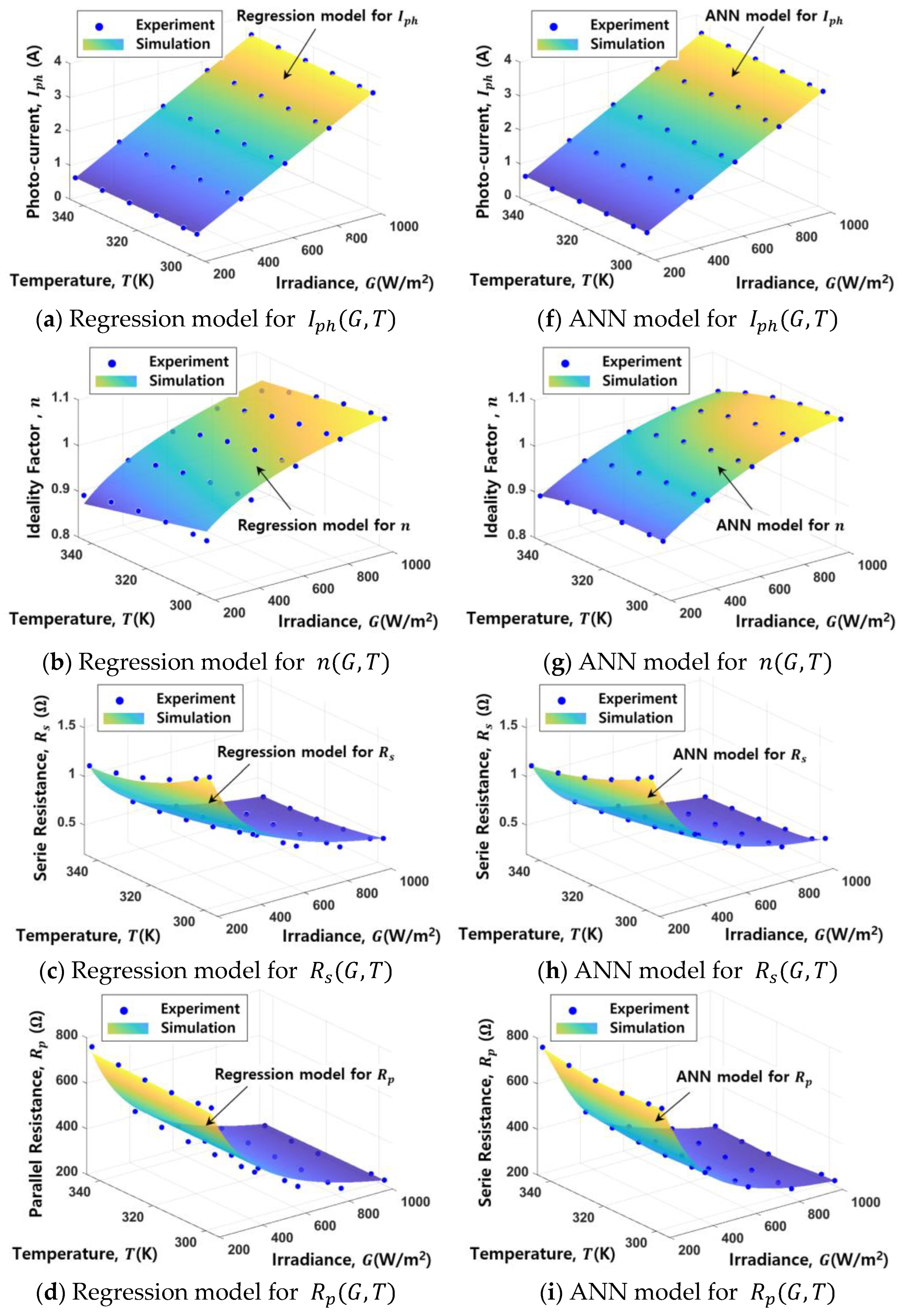
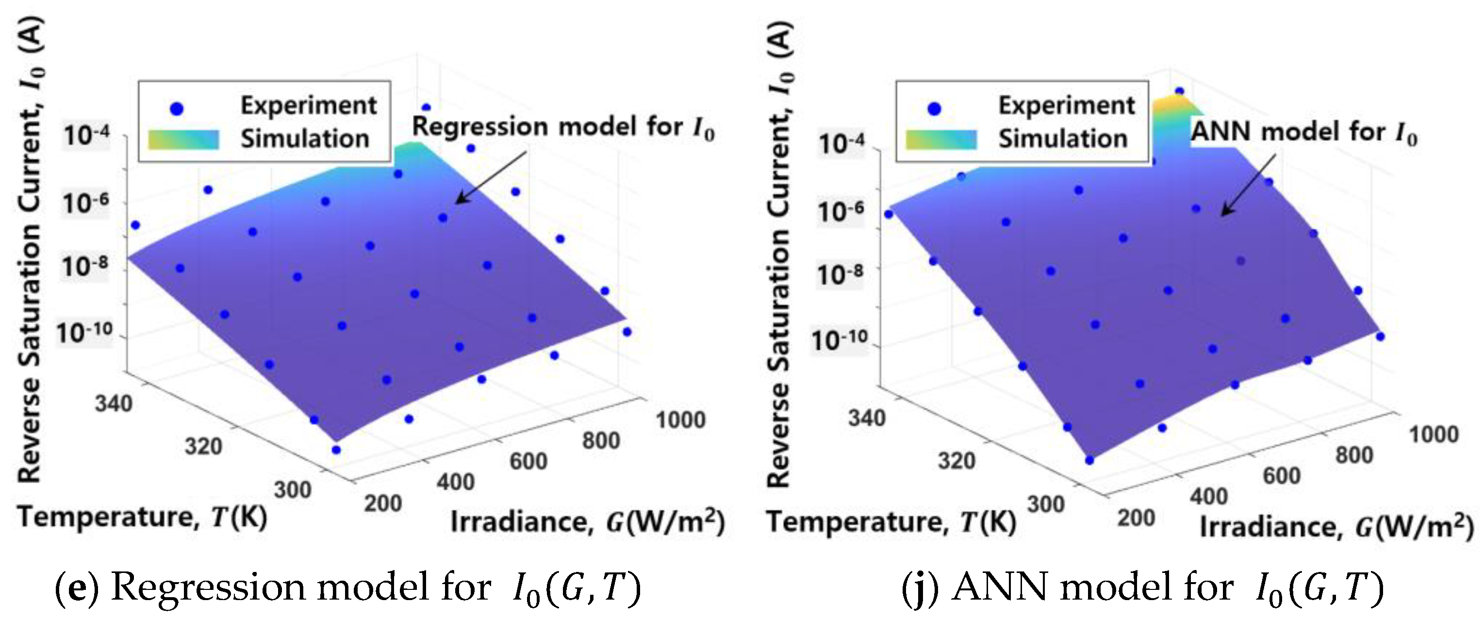
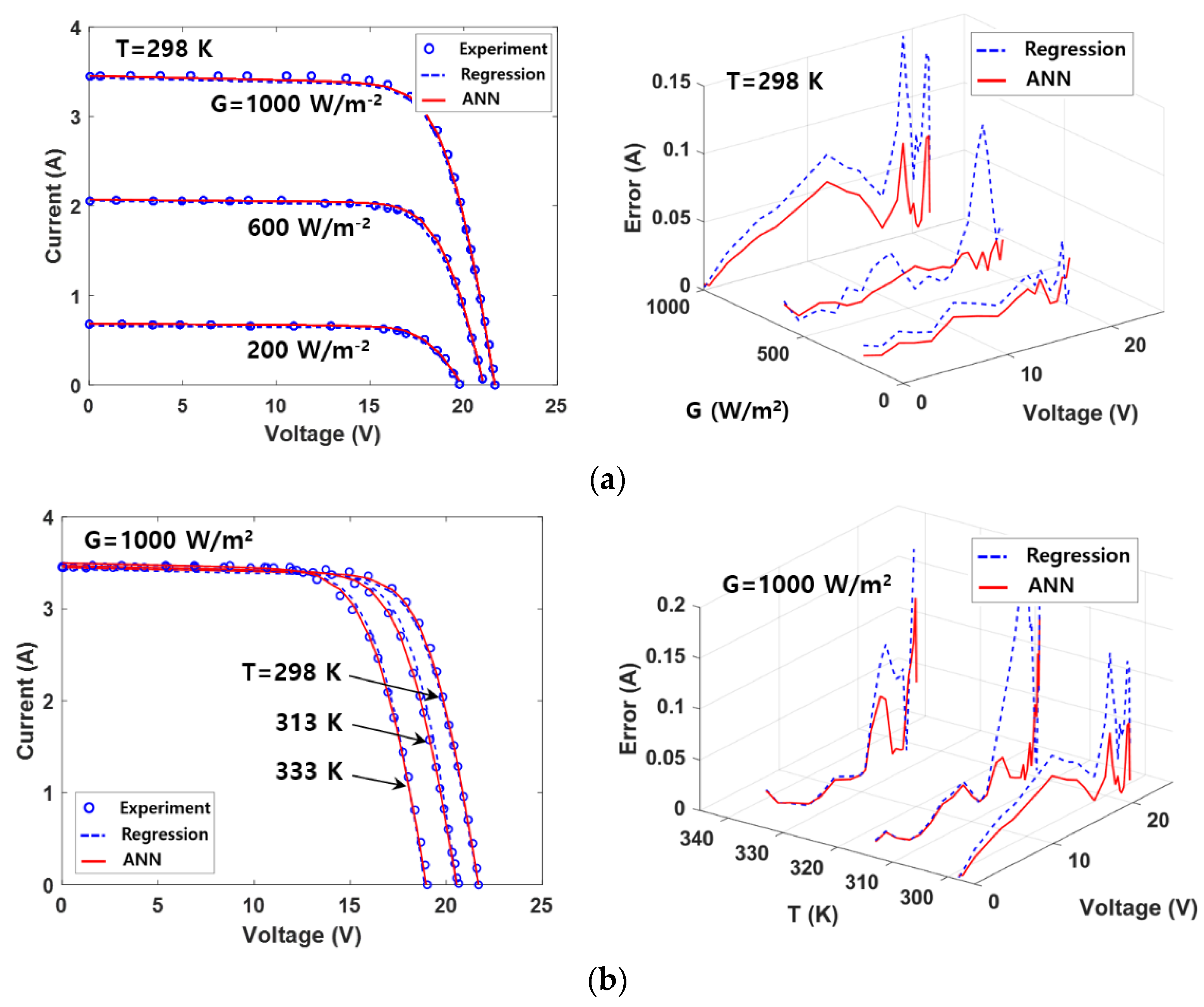
4. Model Verification

The validation of the regression and ANN models for the five parameters ($I_{ph}$,$n$,$R_s$,$R_p$,$I_0$) is assessed by using the experimental data of the monocrystalline SM55 PV panel $\left(N_s=36\right)$ [1]. The five parameters are extracted by using the quality factor variation method from the manufacturer’s data sheet [1,17]. After determining the parameters at standard test conditions ($G_0=1000 \mathrm{W}/{\mathrm{m}}^2$, $T_0=298\mathrm{K}$), the procedure is applied to estimate variations in the five parameters for different temperature levels $\left(T=298~343\mathrm{K}\right)$ and solar irradiance levels $\left(G=200~1000 \mathrm{W}/{\mathrm{m}}^2\right)$. The database obtained from the procedure is used to develop the multiple regression models for $I_{ph}\left(G,T\right)$, $n\left(G,T\right)$, $R_s\left(G,T\right)$, $R_s\left(G,T\right)$, and $I_0\left(G,T\right)$.

Table 1. Regression model and $R^2$ for parameters estimated from experimental data.

Parameters	$\mathbf{Regression}\mathbf{Models}\mathbf{and}{\mathit{R}}^2$
$I_{ph}\left(G,T\right) \left(\mathrm{A}\right)$	$\left(\frac{G}{G_0}\right)\left[3.457+1.407\times {10}^{-3}\left(T-T_0\right)\right]$, $R^2=1.000$
$V_{oc}\left(G,T\right) \left(\mathrm{V}\right)$	$21.63\left[1-3.434\times {10}^{-3}\left(T-T_0\right)+1.752\times {10}^{-4}{V}_t\ln \left(\frac{G}{G_0}\right)\right]$, $R^2=0.9985$
$n\left(G,T\right)$	$1.084\left[1-8.455\times {10}^{-4}\left(T-T_0\right)+2.749\times {10}^{-4}{V}_t\ln \left(\frac{G}{G_0}\right)\right]$, $R^2=0.96$92
$R_s\left(G,T\right) \left(\mathrm{\Omega }\right)$	$0.4724\frac{1+1.405\times {10}^{-2}+6.854\times {10}^{-4}{V}_t\ln \left(\frac{G}{G_0}\right)}{\left(\frac{G}{G_0}\right)\left[1+3.488\times {10}^{-2}\left(T-T_0\right)\right]}$, $R^2=0.99$38
$R_p\left(G,T\right) \left(\mathrm{\Omega }\right)$	$222\frac{1+1.890\times {10}^{-2}+7.246\times {10}^{-4}{V}_t\ln \left(\frac{G}{G_0}\right)}{\left(\frac{G}{G_0}\right)\left[1+2.515\times {10}^{-2}\left(T-T_0\right)\right]}$, $R^2=0.9926$
$I_0\left(G,T\right) \left(\mathrm{A}\right)$	$\left[I_{ph}\left(G,T\right)-\frac{V_{oc}\left(G,T\right)}{R_p\left(G,T\right)}\right]/\left[\exp \left(\frac{V_{oc}\left(G,T\right)}{n\left(G,T\right)V_t}\right)-1\right]$

shows the regression models and coefficient of determination $R^2$ estimated by using Equations (4)–(9). As shown in Table 1, the regression models have a high coefficient of determination ($R^2=0.9692~1.000)$, and $I_0\left(G,T\right)$ is obtained by other parameters with a high coefficient of determination.

The best ANN model has an input layer with two variables, two hidden layers with five neurons in each layer, and an output layer with five variables (2-5-5-5 topology). Logarithm data preprocessing is used to improve the ANN model accuracy for the reverse saturation current $I_0\left(G,T\right)$. For training the ANN model, the offline method is utilized to generate the dataset for the five parameters of the PV panel, which is extracted from manufacturer’s data sheet. Figure 3 shows the dependence of five parameters on temperature and solar irradiance for the regression model and ANN model. The correlation coefficients are employed to evaluate the accuracy of the ANN model for the five parameters, including the training, validation, and testing phases. As a result, the correlation coefficients with values greater than 99.85% were observed between the predicted and measured data in all network phases.

As plotted in Figure 4, two different statistical metrics based on the measured and estimated five parameters are employed to compare the accuracy of the ANN model with the regression model, including root mean squared error (RMSE) and mean absolute percentage error (MAPE), as follows [14,15]:

$$RMSE=\sqrt{\frac{1}{n}{\displaystyle \sum }_{i=1}^n{\left(y_{m,i}-y_{e,i}\right)}^2}$$

(17)

$$MAPE=\frac{1}{n}{\displaystyle \sum }_{i=1}^n\left|\frac{y_{m,i}-y_{e,i}}{y_{m,i}}\right|\times 100 \left(\%\right)$$

(18)

where $y_{m,i}$ and $y_{e,i}$ are the measured and estimated values, respectively. Both RMSE and MAPE values of the ANN models are lower than those of the regression models. This is attributed to the strong capability of MLP–ANN models to learn the nonlinear relationship between the inputs and the outputs, whereas the regression models may be limited to a specific condition. Figure 5a,b show I–V characteristics and the absolute error by simulated and experimental data at different irradiances and temperatures, respectively. It is found that the absolute error values of the ANN models are lower than the regression models, resulting from the better performance of the ANN models for the five parameters shown in Figure 3.

Table 2. Comparison of maximum absolute errors estimated from different models.

Temperature T (K)	Irradiance G (W/m2)	Maximum Absolute Errors (A) of I–V Curves for SM55 Panel
		Proposed ANN Model	Model 1 [1]	Model 2 [4]	Model 3 [46]
298	200	0.02	0.03	0.03	0.08
	600	0.01	0.04	0.06	0.05
	1000	0.06	0.08	0.06	0.06
298	1000	0.04	0.07	0.06 (293 K)	0.10 (293 K)
313		0.09	0.16	0.15	0.09
333		0.09	0.12	0.10	0.20

shows the comparison of maximum absolute errors of the I–V curves estimated from the proposed ANN model and different models for the SM55 PV panel. As can be seen, the maximum absolute errors of the proposed ANN model are much lower than the other models for different irradiances and temperatures. These results justify the higher accuracy of the ANN models, compared with other works [1,4,46].

5. Conclusions

The electrical characteristics of a PV module under arbitrary operating conditions have been estimated by using the regression and ANN models. The models are utilized to predict the five parameters of a single diode solar cell, and the parameters are combined with an explicit equation for I–V characteristics. The inputs of the regression and ANN models are temperature and solar irradiance, while the outputs are the five parameters. The dataset needed for the five parameters was extracted from manufacturer’s data sheet and used to construct the regression and ANN models. The best neural network architecture had a 2-5-5-5 topology for the five parameters, leading to correlation coefficients with values greater than 99.85%. Both the RMSE and MAPE values of the ANN models were found to be lower than those of the regression models. With comparative results, the ANN models show better performance than the regression models in predicting I–V characteristics under varying temperature and solar irradiance. It is applicable to extend the higher capability of ANN models to the prediction of electrical characteristics for diverse solar cells under actual weather conditions.

References

1. Zaimi, M.; Achouby, E.; Ibral, A.; Assaid, E.M. Determining combined effects of solar radiation and panel junction temperature on all model-parameters to forecast peak power and photovoltaic yield of solar panel under non-standard conditions. Sol. Energy 2019, 191, 341–359. [Google Scholar] [CrossRef]
2. Ibrahim, H.; Anani, N. Variations of PV module parameters with irradiance and temperature. Energy Procedia 2017, 134, 276–285. [Google Scholar] [CrossRef]
3. Teh, C.T.Q.; Drieberg, M.; Soeung, S.; Ahmad, R. Simple PV modeling under variable operating conditions. IEEE Access 2021, 9, 96546–96558. [Google Scholar] [CrossRef]
4. Dongue, S.B.; Njomo, D.; Ebengai, L. An improved nonlinear five-point model for photovoltaic modules. Int. J. Photoenergy 2013, 2013, 680213-1-11. [Google Scholar]
5. Shinong, W.; Qianlong, M.; Jie, X.; Yuan, G.; Shilin, L. An improved mathematical model of photovoltaic cells based on datasheet information. Sol. Energy 2020, 199, 437–446. [Google Scholar] [CrossRef]
6. Brano, V.L.; Orioli, A.; Ciulla, G.; Gangi, A.D. An improved five parameter model for photovoltaic modules. Sol. Energy Mater. Sol. Cells 2010, 94, 1358–1370. [Google Scholar] [CrossRef]
7. Anani, N.; Ibrahim, H. Adjusting the single-diode model parameters of a photovoltaic module with irradiance and temperature. Energies 2020, 13, 3326. [Google Scholar] [CrossRef]
8. Hao, P.; Zhang, Y.; Lu, H.; Lang, Z. A novel method for parameter identification and performance estimation of PV module under varying operation conditions. Energy Convers. Manag. 2021, 247, 114689. [Google Scholar] [CrossRef]
9. Deng, J.; Wang, Y. Research on MPPT of photovoltaic system based on PSO with time-varying compression factor. IEICE Electron. Express 2022, 19, 20220165. [Google Scholar] [CrossRef]
10. Wang, Y.; Zhang, B.; Yang, Y.; Wen, H.; Zhang, Y.; Chen, X. A new optimized control system architecture for solar photovoltaic energy storage application. IEICE Electron. Express 2021, 18, 20200404. [Google Scholar] [CrossRef]
11. Carrasco, J.A.; de Quiros, F.G.; Alaves, H.; Navalon, M. A PWM multiplier for maximum power point estimation of a solar panel. IEICE Electron. Express 2018, 15, 20180496. [Google Scholar] [CrossRef]
12. Liu, H.D.; Lin, C.H.; Lu, S.D. A novel MPPT algorithm considering solar photovoltaic modules and load characteristics for a single stage standalone solar photovoltaic system. IEICE Electron. Express 2020, 17, 20200099. [Google Scholar] [CrossRef]
13. Picault, D.; Raison, B.; Bacha, S.; de la Casa, J.; Aguilera, J. Forecasting photovoltaic array power production subject to mismatch losses. Sol. Energy 2010, 84, 1301–1309. [Google Scholar] [CrossRef]
14. Jain, A.; Sharma, S.; Kapoor, A. Solar cell array parameters using Lambert W-function. Sol. Energy Mater. Sol. Cells 2006, 90, 25–31. [Google Scholar] [CrossRef]
15. Fathabadi, H. Lambert W function-based technique for tracking the maximum power point of PV modules connected in various configurations. Renew. Energy 2015, 74, 214–226. [Google Scholar] [CrossRef]
16. Hmamou, D.B.; Elyaqouti, M.; Arjdal, E.; Ibrahim, A.; Abdul-Ghaffar, H.I.; Aboelsaud, R.; Obukhov, S.; Diab, A.A.Z. Parameters identification and optimization of photovoltaic panels under real conditions using Lambert W-function. Energy Rep. 2021, 7, 9035–9045. [Google Scholar] [CrossRef]
17. Achouby, E.; Zaimi, M.; Ibral, A.; Assaid, E.M. New analytical approach for modelling effects of temperature and irradiance on physical parameters of photovoltaic solar module. Energy Convers. Manag. 2018, 177, 258–271. [Google Scholar] [CrossRef]
18. Silva, E.A.; Bradaschia, F.; Cavalcanti, M.C.; Nascimento, A.J.; Michels, L., Jr.; Pietta, L.P. An eight-parameter adaptive model for the single diode equivalent circuit based on the photovoltaic module’s physics. IEEE J. Photovolt. 2017, 7, 1115–1123. [Google Scholar] [CrossRef]
19. Zhang, C.; Zhang, Y.; Su, J.; Gu, T.; Yang, M. Modeling and prediction of PV module performance under different operating conditions based on power-law I-V model. IEEE J. Photovolt. 2020, 10, 1816–1827. [Google Scholar] [CrossRef]
20. Hejri, M.; Mokhtari, H. On the comprehensive parameterization of the photovoltaic cells and modules. IEEE J. Photovolt. 2017, 7, 250–258. [Google Scholar] [CrossRef]
21. Silva, A.; Bradaschia, F.; Cavalcanti, M.C.; Nascimento, A.J. Parameter estimation method to improve the accuracy of photovoltaic electrical model. IEEE J. Photovolt. 2016, 6, 278–285. [Google Scholar] [CrossRef]
22. Mittal, M.; Bora, B.; Saxena, S.; Gaur, A.M. Performance prediction of PV module using electrical model and artificial neural network. Sol. Energy 2018, 176, 104–117. [Google Scholar] [CrossRef]
23. Karamirad, M.; Omid, M.; Alimardani, R.; Mousazadeh, H.; Heidari, S.N. ANN based simulation and experimental verification of analytical four- and five-parameters models of PV modules. Simul. Model. Pract. Theory 2013, 34, 86–98. [Google Scholar] [CrossRef]
24. Zhu, H.; Lu, L.; Yao, J.; Dai, S.; Hu, Y. Fault diagnosis approach for photovoltaic arrays based on unsupervised sample clustering and probabilistic neural network model. Sol. Energy 2018, 176, 395–405. [Google Scholar] [CrossRef]
25. Chine, W.; Mellit, A.; Lughi, V.; Malek, A.; Sulligoi, G.; Massi Pavan, A. A novel fault diagnosis technique for photovoltaic systems based on artificial neural networks. Renew. Energy 2016, 90, 501–512. [Google Scholar] [CrossRef]
26. Li, B.; Delpha, C.; Diallo, D.; Migan-Dubois, A. Application of artificial neural networks to photovoltaic fault detection and diagnosis: A review. Renew. Sustain. Energy Rev. 2021, 138, 110512. [Google Scholar] [CrossRef]
27. Zecevic, Z.; Rolevski, M. Neural network approach to MPPT control and irradiance estimation. Appl. Sci 2020, 10, 5051. [Google Scholar] [CrossRef]
28. Karatepe, E.; Boztepe, M.; Colak, M. Neural network based solar cell model. Energy Convers. Manage. 2006, 47, 1159–1178. [Google Scholar] [CrossRef]
29. Xu, E.; Zhang, X.; Huang, Z.; Xie, S.; Gu, W.; Wang, X.; Zhang, L.; Zhang, Z. Current characteristics estimation of Si PV modules based on artificial neural network modeling. Materials 2019, 12, 3037. [Google Scholar] [CrossRef] [Green Version]
30. Chikh, A.; Chandra, A. Adaptive neuro-fuzzy based solar cell model. IET Renew. Power Gener. 2014, 8, 679–686. [Google Scholar] [CrossRef]
31. Rizzo, S.A.; Scelba, G. ANN based MPPT method for rapidly variable shading conditions. Appl. Energy 2015, 145, 124–132. [Google Scholar] [CrossRef]
32. Cortes, B.; Sanchez, R.T.; Flores, J.J. Characterization of polycrystalline photovoltaic cell using artificial neural network. Sol. Energy 2020, 196, 157–167. [Google Scholar] [CrossRef]
33. Elsheikh, A.H.; Sharshir, S.W.; Elaziz, M.A.; Kabeel, A.E.; Guilan, W.; Haiou, Z. Modeling of solar energy systems using artificial neural network: A comprehensive review. Sol. Energy 2019, 180, 622–639. [Google Scholar] [CrossRef]
34. Kalogirou, S.A.; Mathioulakis, E.; Belessiotis, V. Artificial neural network for the performance prediction of large solar systems. Renew. Energy 2014, 63, 90–97. [Google Scholar] [CrossRef]
35. Castro, R. Data-driven PV modules modelling: Comparison between equivalent electric circuit and artificial intelligence based models. Sustain. Energy Technol. Assess. 2018, 30, 230–238. [Google Scholar] [CrossRef]
36. Celik, A.N. Artificial neural network modelling and experimental verification of the operating current of mono-crystalline photovoltaic modules. Sol. Energy 2011, 85, 2507–2517. [Google Scholar] [CrossRef]
37. Almonacid, F.; Rus, C.; Hontoria, L.; Munoz, F.J. Characterization of PV CIS module by artificial neural networks. A comparative study with other methods. Renew. Energy 2010, 35, 973–980. [Google Scholar] [CrossRef]
38. Huang, C.; Bensoussan, A.; Edesess, M.; Tsui, K.L. Improvement in artificial neural network-based estimation of grid connected photovoltaic power output. Renew. Energy 2016, 97, 838–848. [Google Scholar] [CrossRef]
39. Bonanno, F.; Capizzi, G.; Graditi, G.; Napoli, C.; Tina, G.M. A radial basis function neural network based approach for the electrical characteristics estimation of a photovoltaic module. Appl. Energy 2012, 97, 956–961. [Google Scholar] [CrossRef] [Green Version]
40. Zhang, L.; Bai, Y.F. Genetic algorithm-trained radial basis function neural networks for modelling photovoltaic panels. Eng. Appl. Artif. Intell. 2005, 18, 833–844. [Google Scholar] [CrossRef]
41. Chen, Z.; Yu, H.; Luo, L.; Wu, L.; Zheng, Q.; Wu, Z.; Cheng, S.; Lin, P. Rapid and accurate modeling of PV modules based on extreme learning machine and large datasets of I–V curves. Appl. Energy 2021, 292, 116929. [Google Scholar] [CrossRef]
42. Liu, Y.H.; Liu, C.L.; Huang, J.W.; Chen, J.H. Neural-network-based maximum power point tracking methods for photovoltaic systems operating under fast changing environments. Sol. Energy 2013, 89, 42–53. [Google Scholar] [CrossRef]
43. Barhmi, S.; Elfatni, O.; Belhaj, I. Forecasting of wind speed using multiple linear regression and artificial neural networks. Energy Syst. 2020, 11, 935–946. [Google Scholar] [CrossRef]
44. Asilturl, I. Predicting surface roughness of hardened AISI 1040 based on cutting parameters using neural networks and multiple regression. Int. J. Adv. Manuf. Technol. 2012, 63, 249–257. [Google Scholar] [CrossRef]
45. Wang, Y.M.; Elhag, T.M.S. A comparison of neural network, evidential reasoning and multiple regression analysis in modelling bridge risks. Expert Syst. Appl. 2007, 32, 336–348. [Google Scholar] [CrossRef]
46. Khalid, C.; Mohammed. F.; Mohcine, M. An accurate modelling of PV modules based on two-diode model. Renew. Energy 2021, 167, 294–305. [Google Scholar]
Figure 1. PV-equivalent circuit of a single diode with series and parallel resistance at arbitrary irradiance (G) and temperature (T).
Electronics 11 04228 g001
Figure 2. Configuration of the proposed photovoltaic model.
Electronics 11 04228 g002
Figure 3. Dependence of the five parameters on temperature and solar irradiance for the regression model (ae) and ANN model (fj).
Electronics 11 04228 g003aElectronics 11 04228 g003b
Figure 4. Statistical metrics for the five parameters in evaluating the accuracy of the regression model and ANN model: (a) RMSE and (b) MAPE.
Electronics 11 04228 g004
Figure 5. I–V curves and absolute error by simulated and experimental data (a) at different irradiances and (b) at different temperatures.
Electronics 11 04228 g005