
Design of an Adaptive Distributed Drive Control Strategy for a Wheel-Side Rear-Drive Electric Bus
Abstract
:1. Introduction
2. Build Dynamics Models
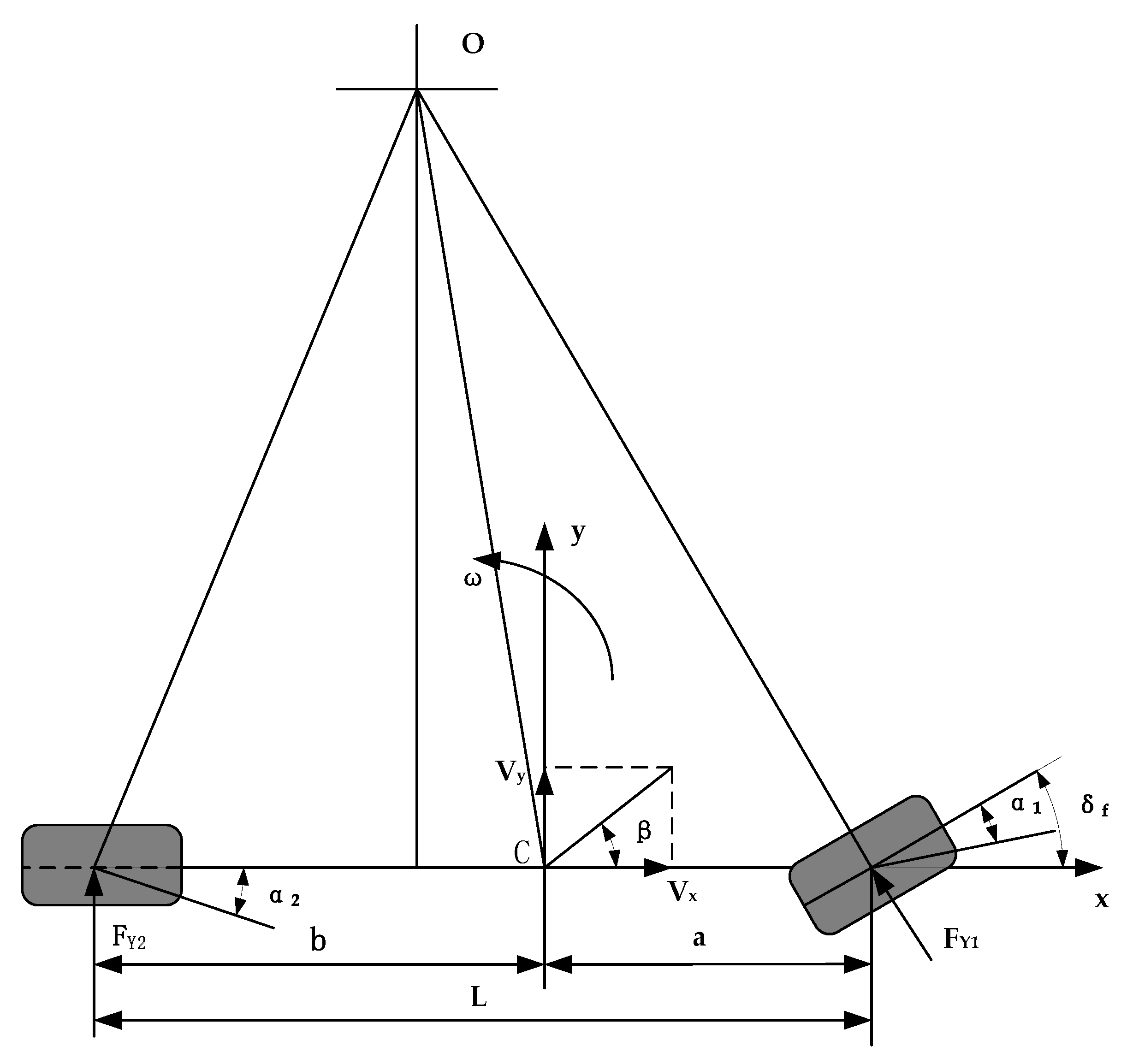
2.1. Reference Model
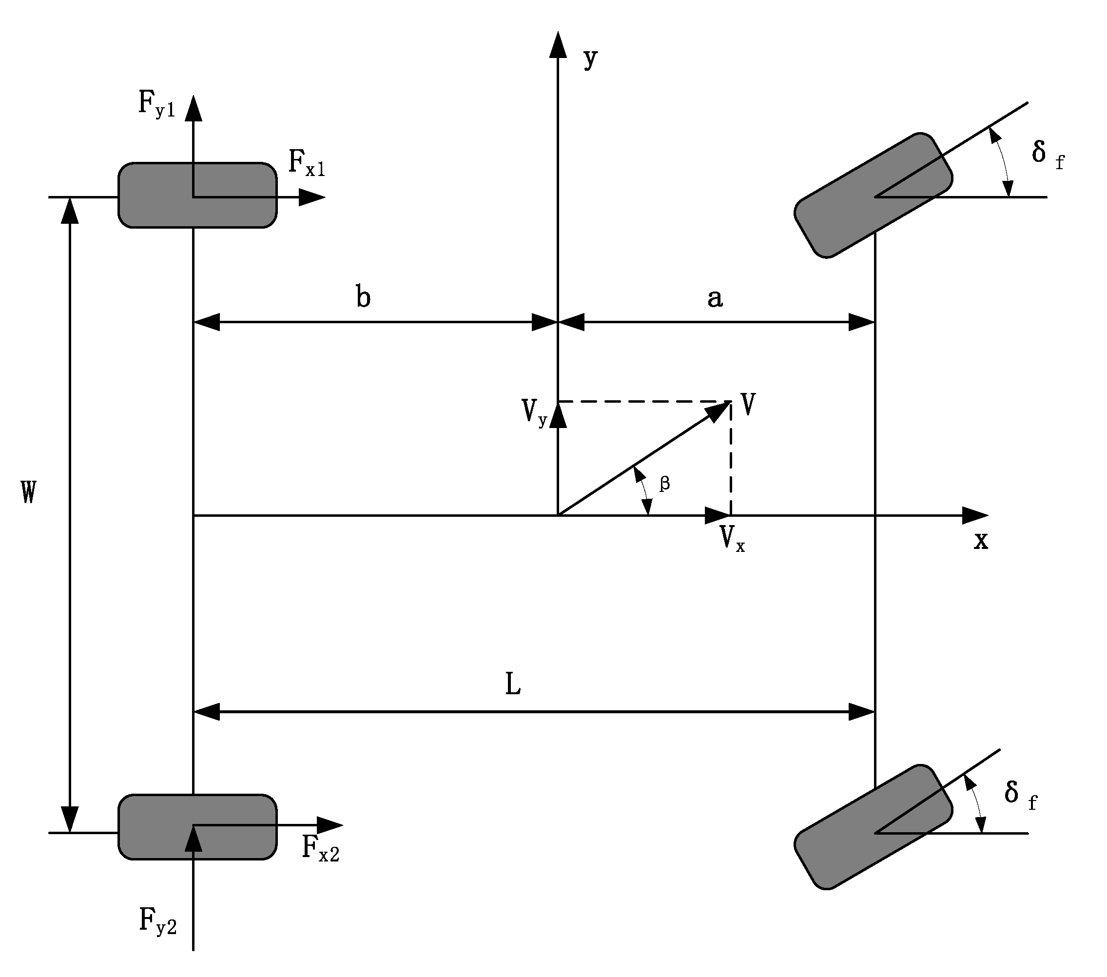
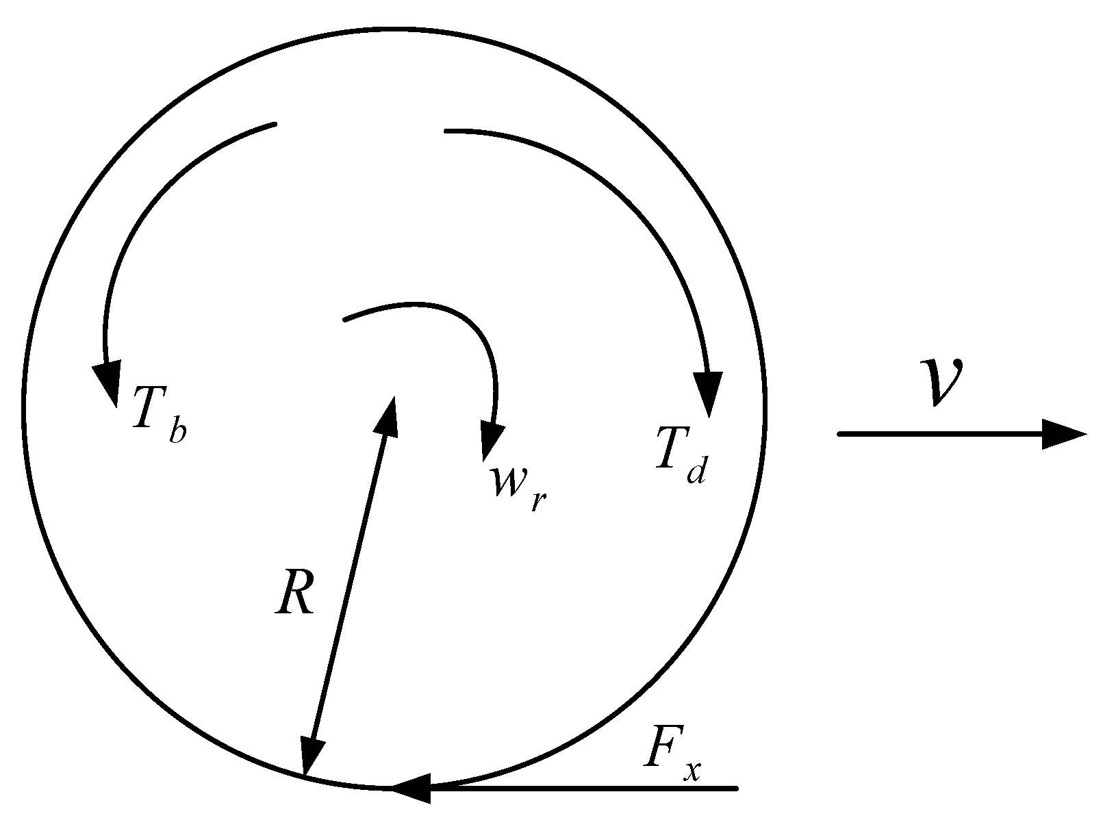
2.2. Vehicle Model
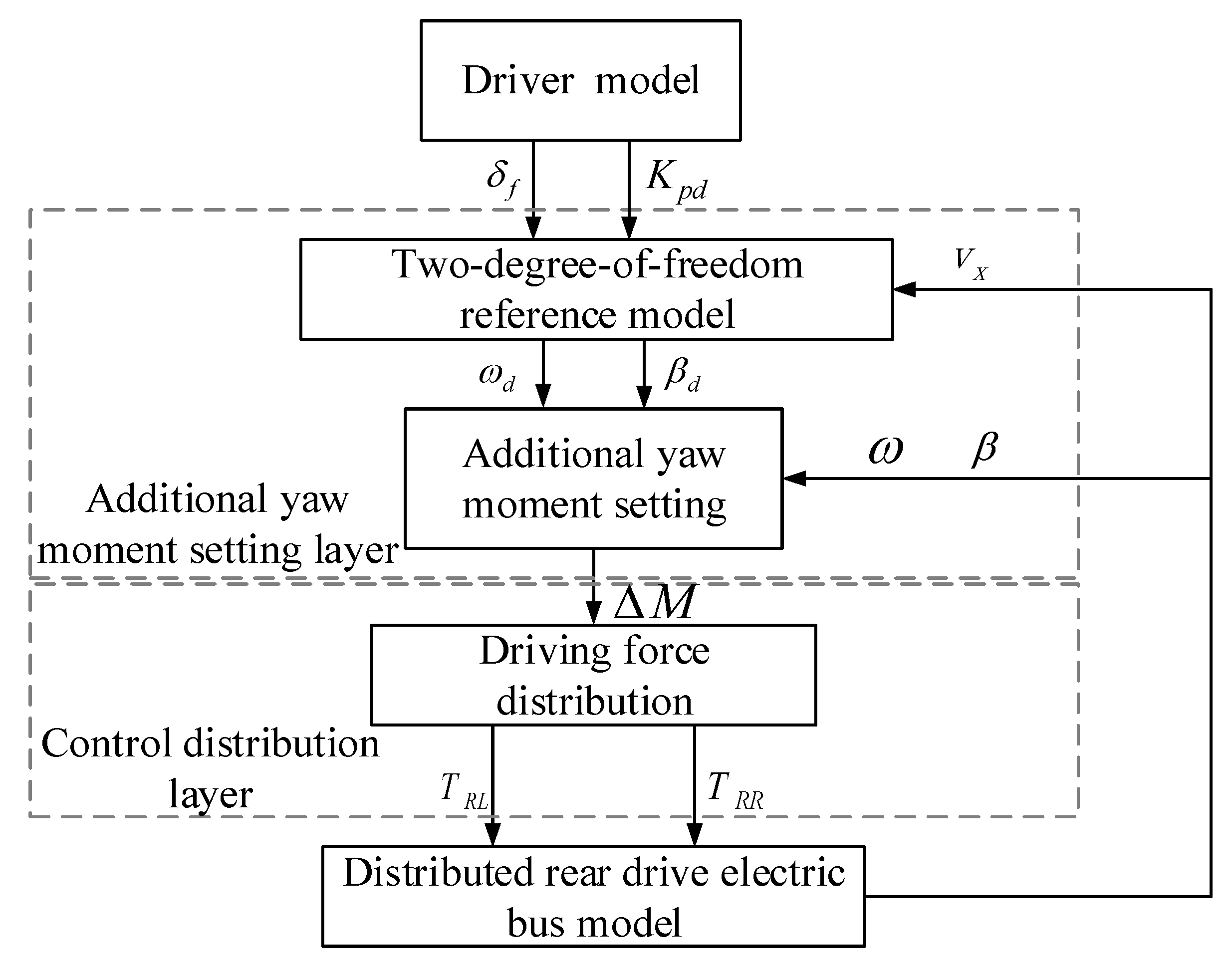
3. Adaptive Distributed Drive Control System Design
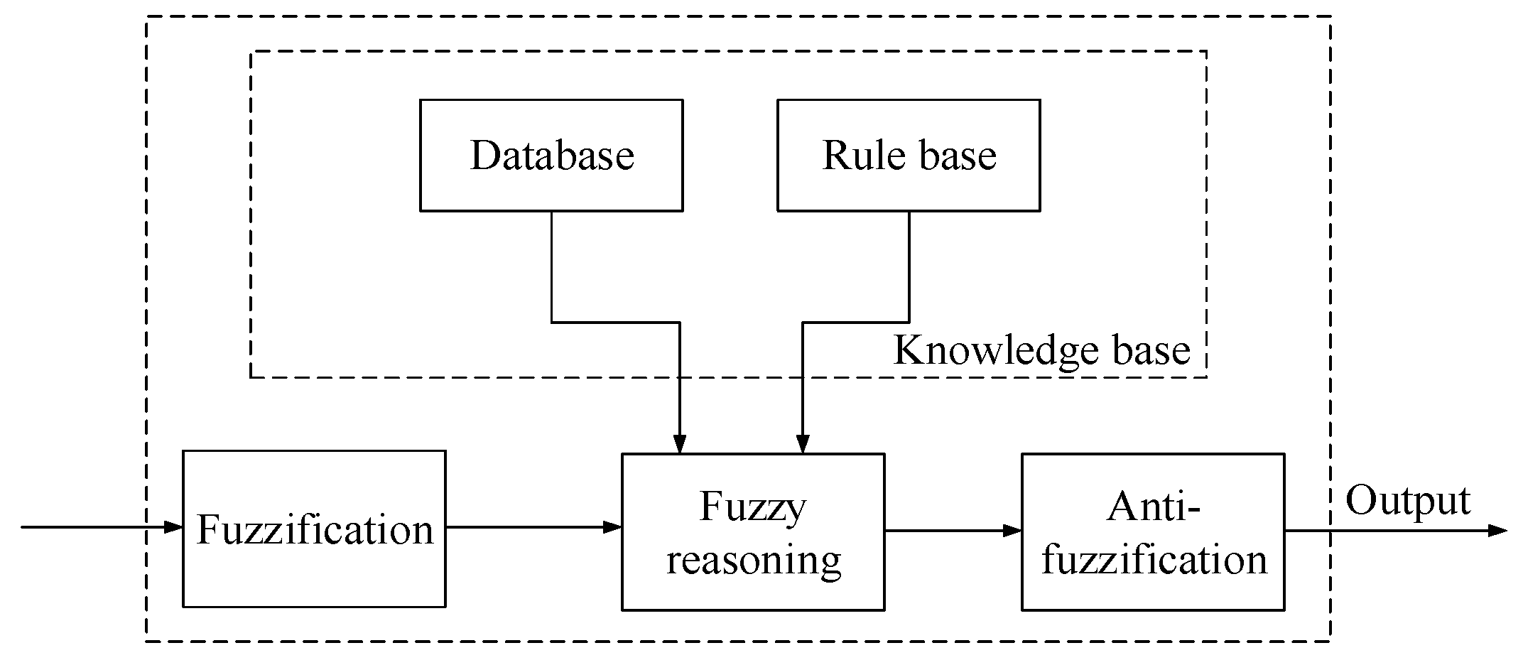
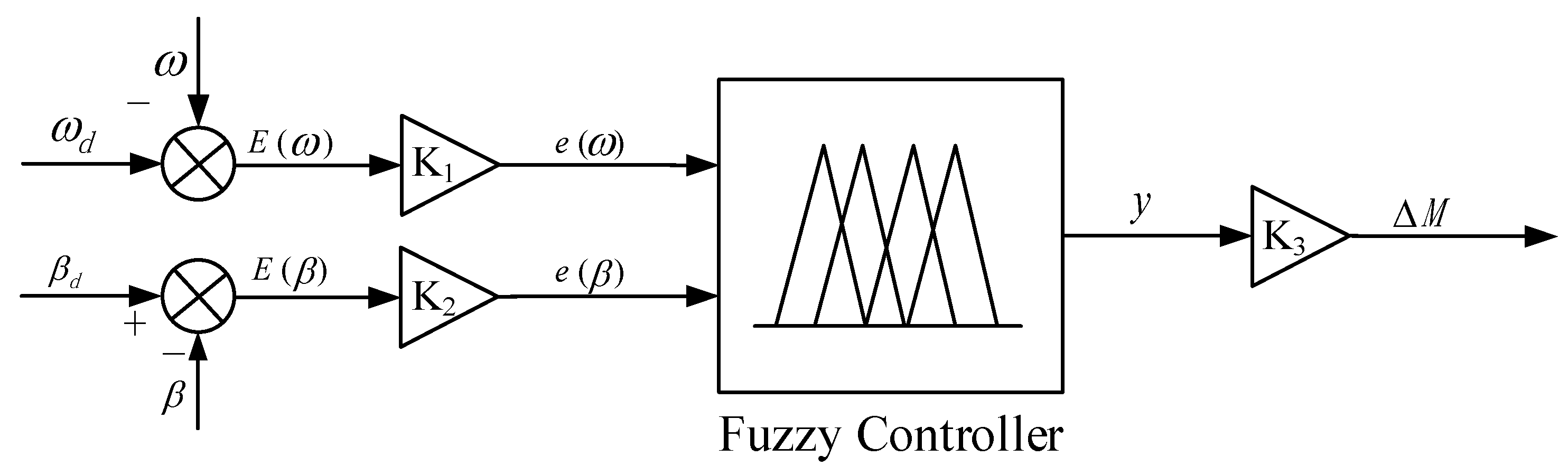
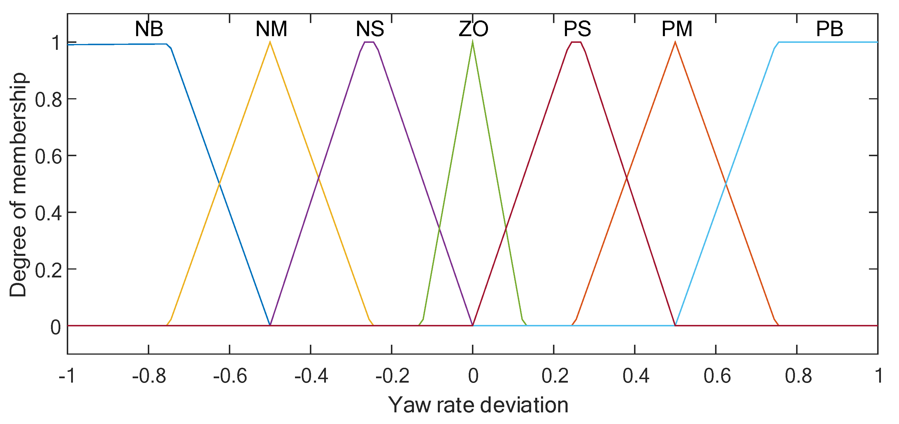
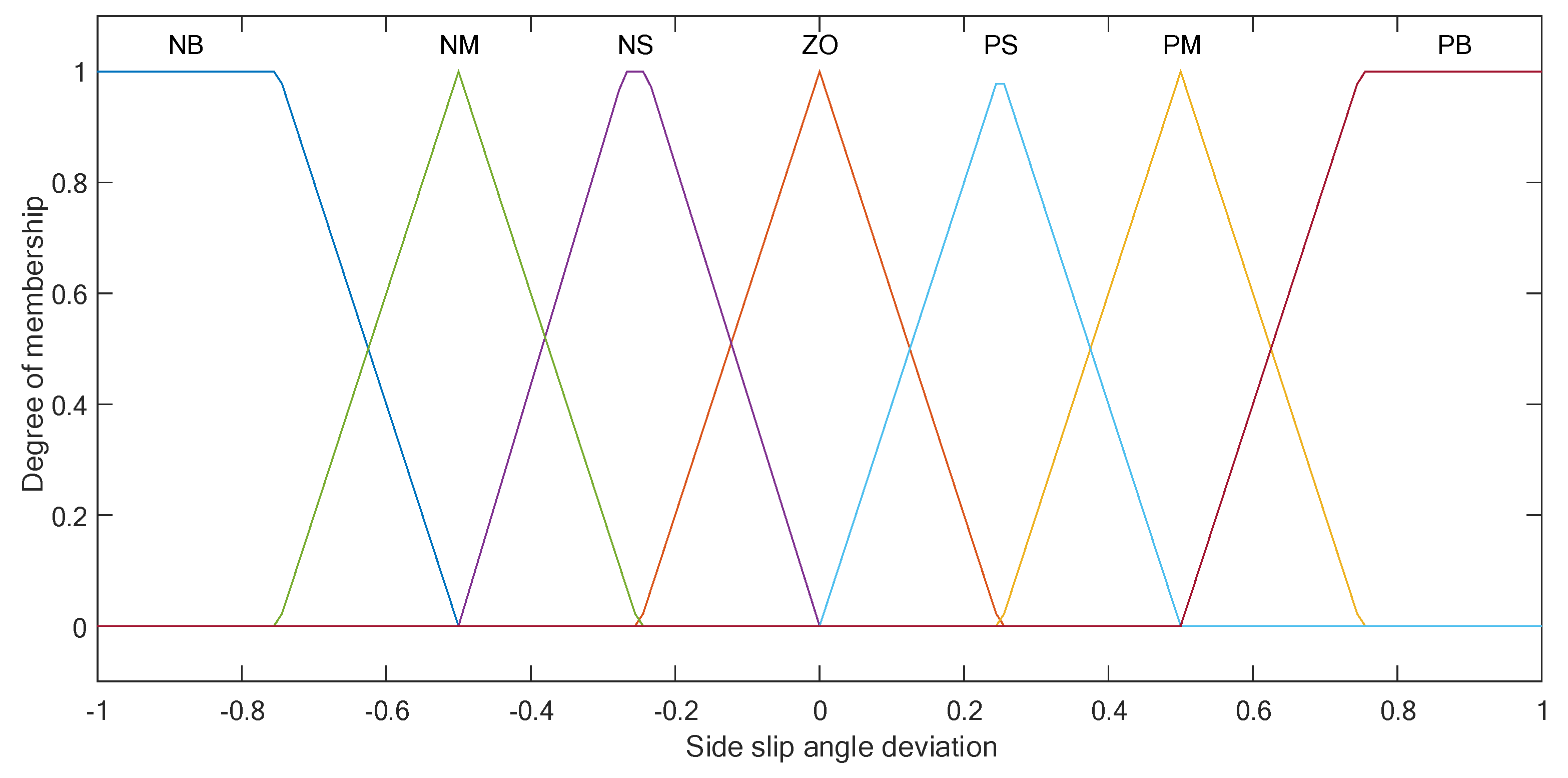
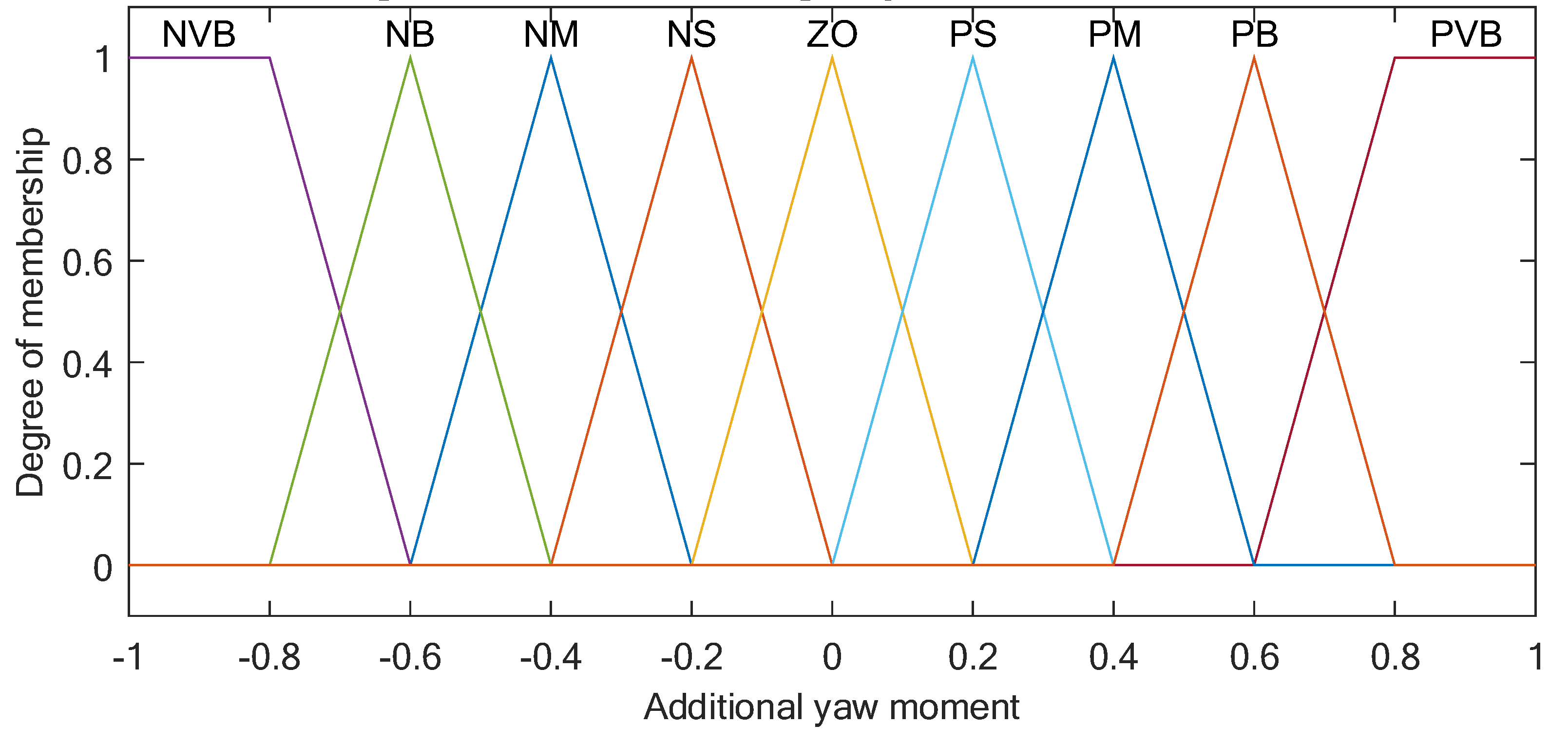
3.1. Additional Yaw Moment Calculation Based on Fuzzy Controller
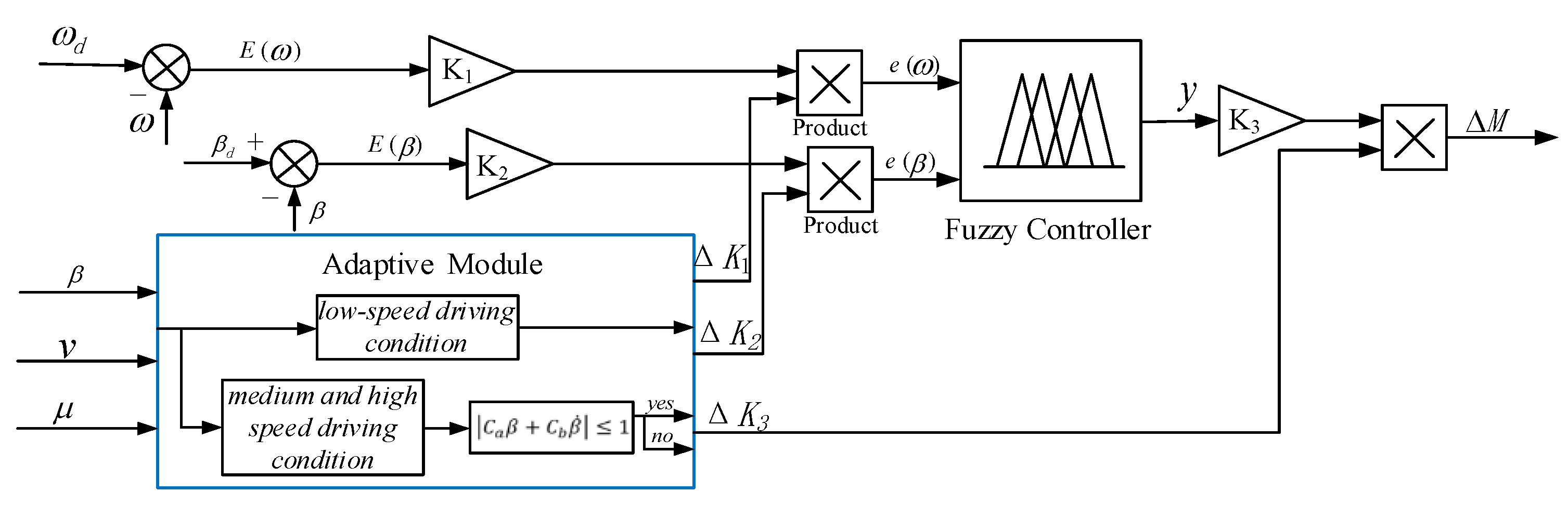
3.2. Additional Yaw Moment Calculation Based on an Adaptive Fuzzy Controller
3.3. Driving Torque Distribution
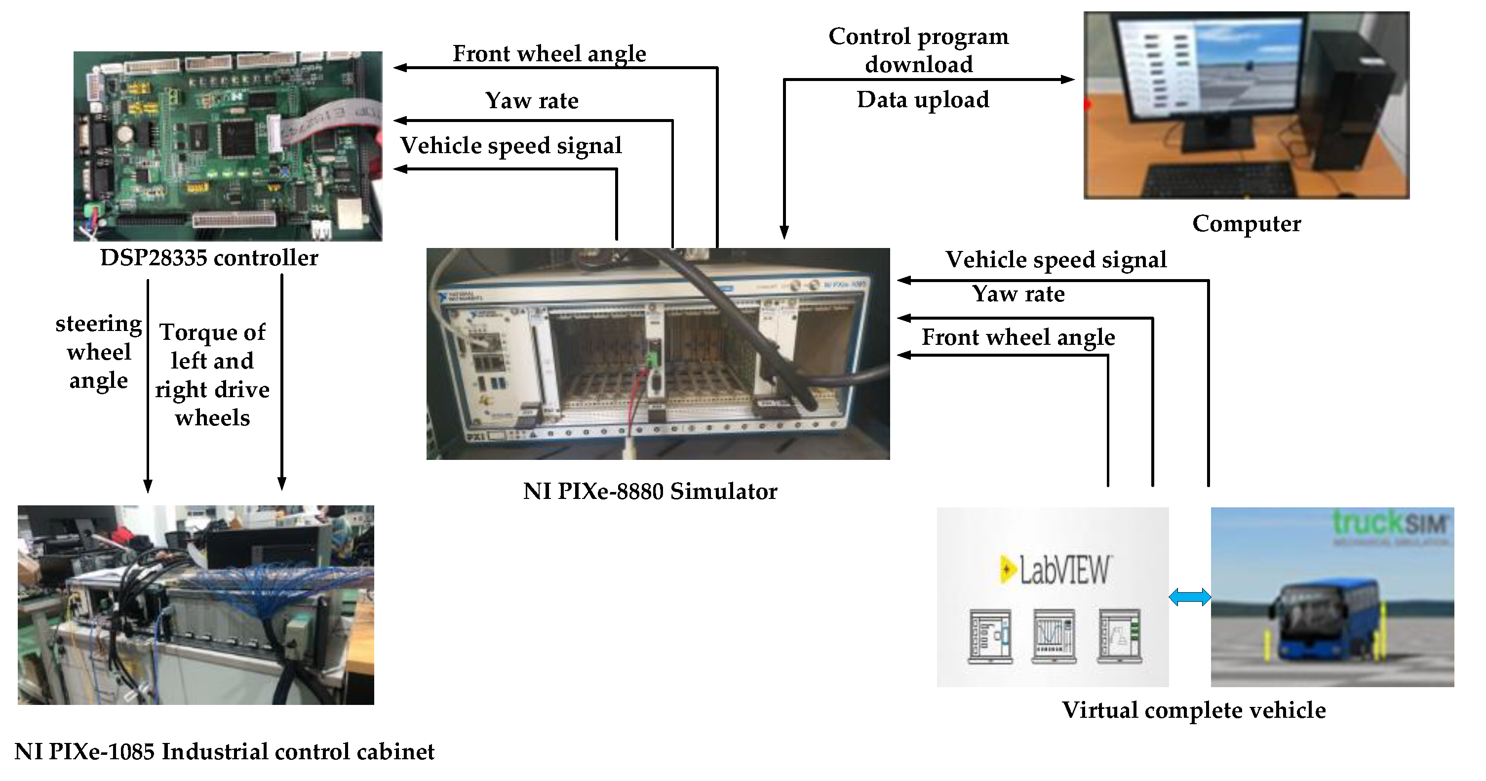
4. Hardware-in-the-Loop Test
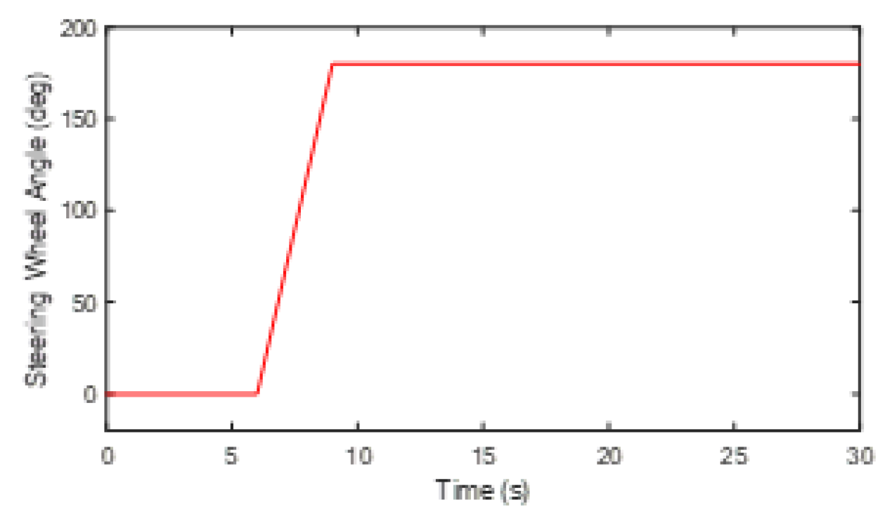
4.1. Large Turning in a Low-Speed Driving Condition
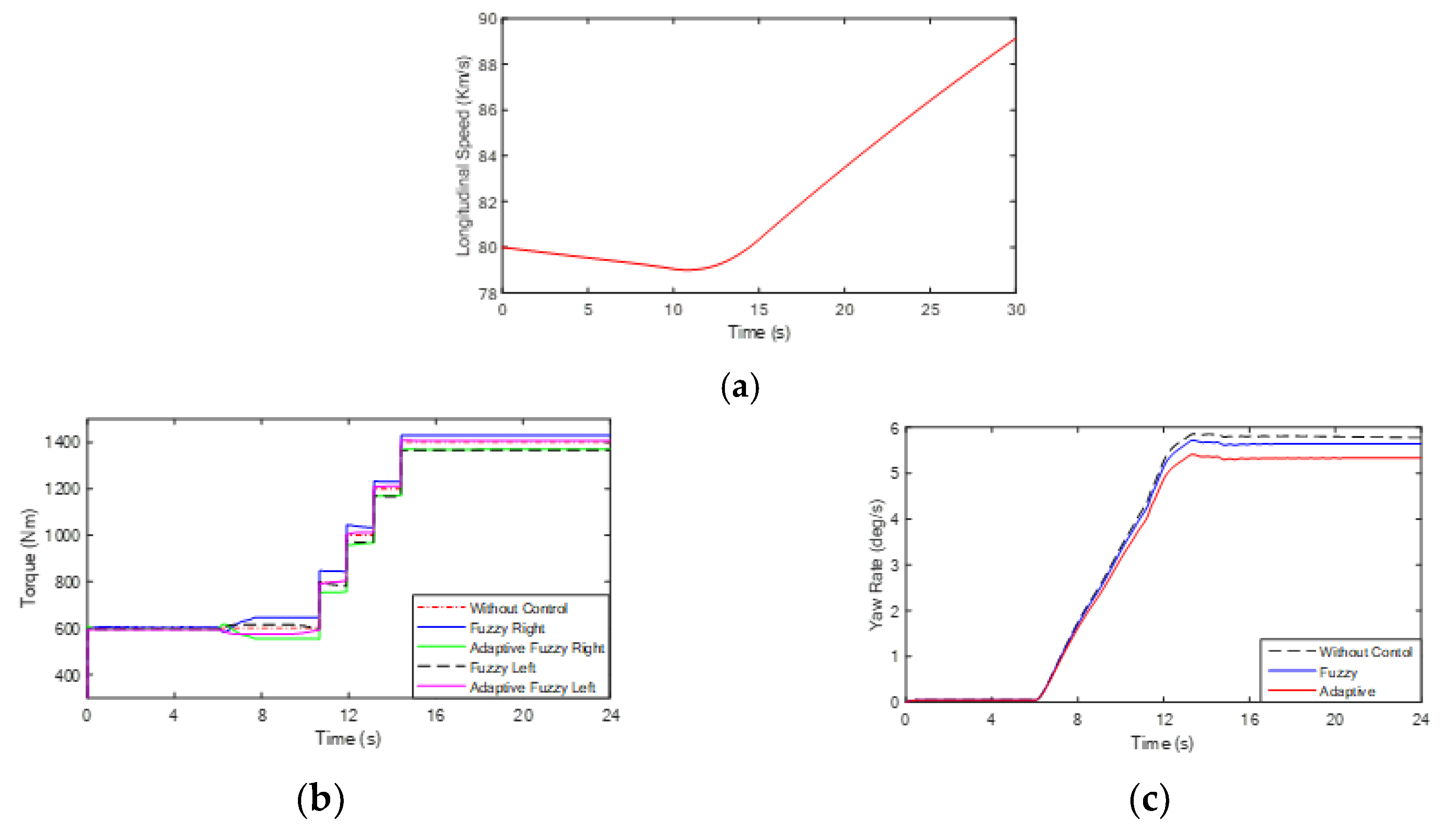
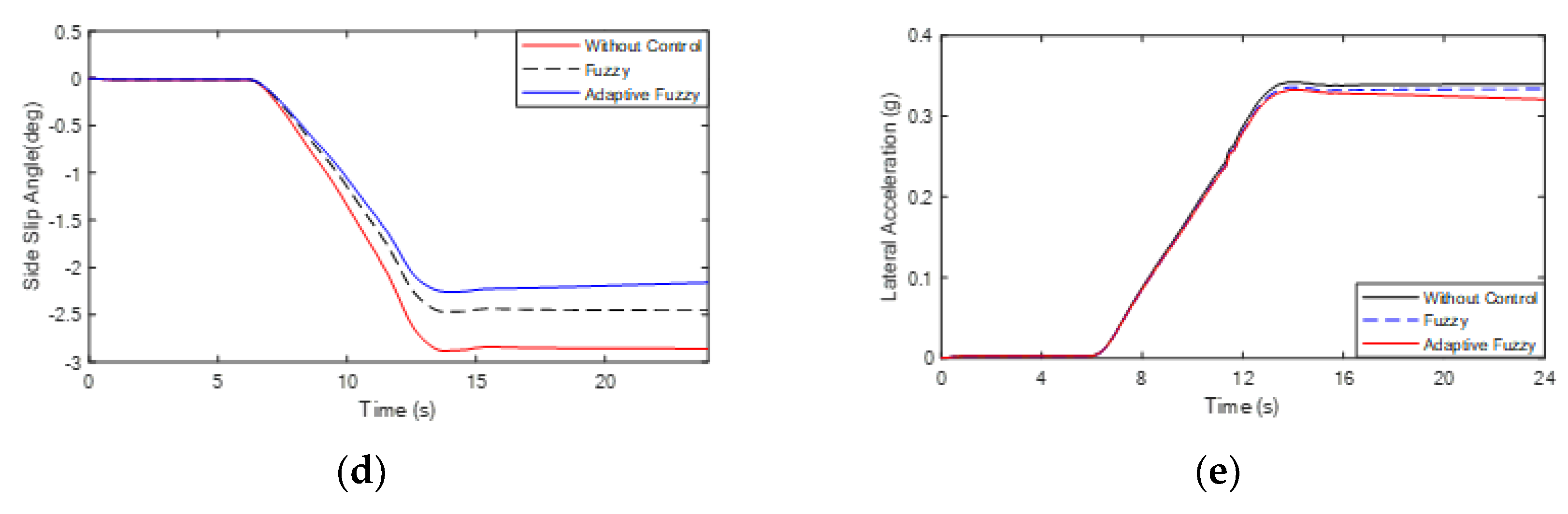
4.2. Small Turning in a High-Speed Driving Condition
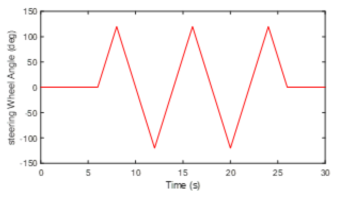
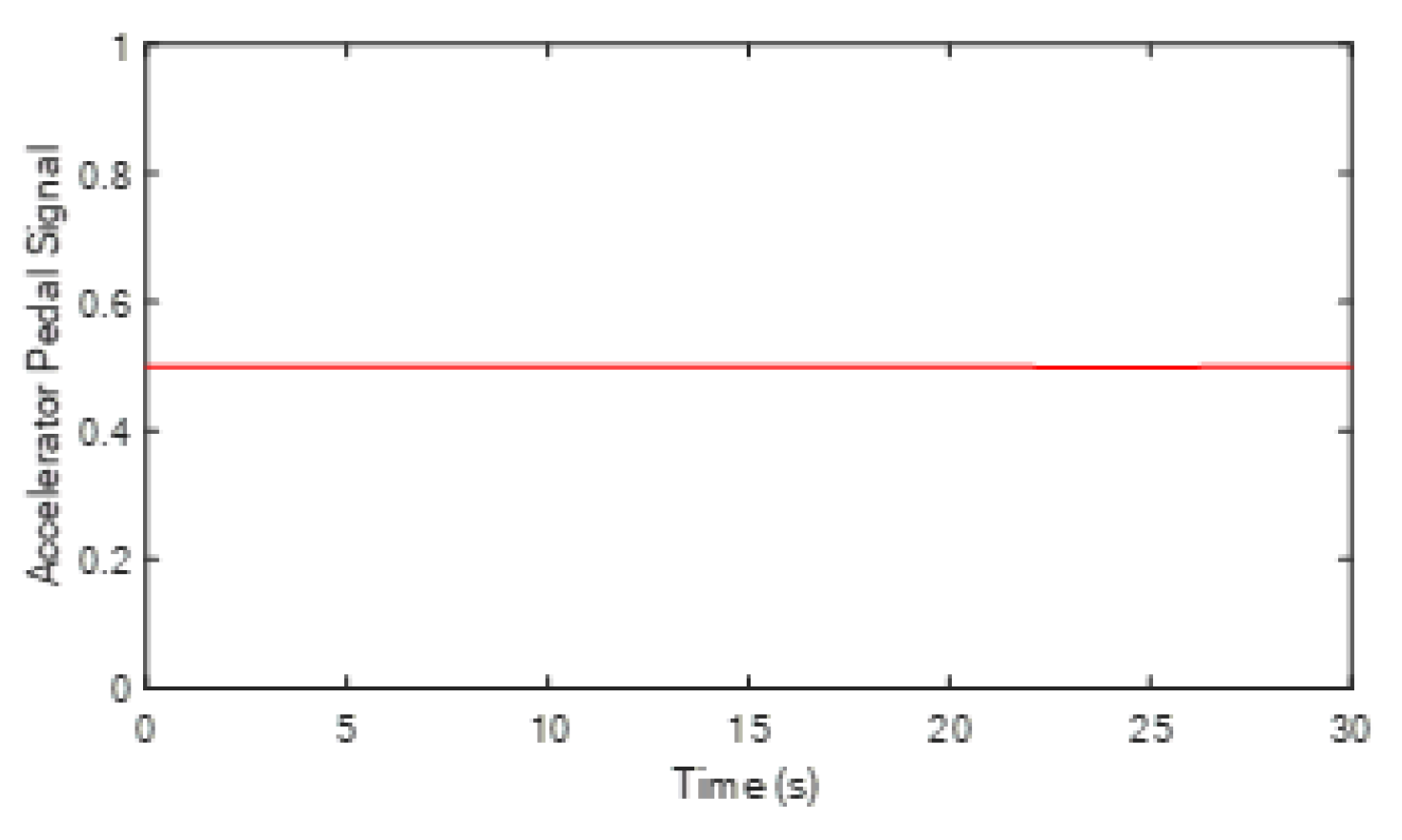
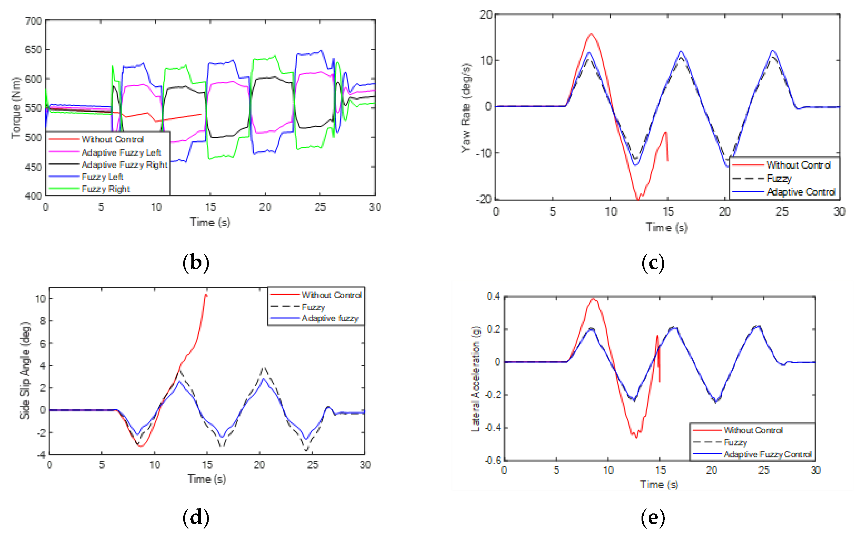
4.3. Slalom Test in a Medium-Speed Driving Condition
5. Conclusions
Author Contributions
Funding
Data Availability Statement
Conflicts of Interest
References
- Koibuchi, K.; Yamamoto, M.; Fukada, Y.; Inagaki, S. Vehicle stability control in limit cornering by active brake. JSAE Review 1996, 16, 323. [Google Scholar]
- Fujimoto, H.; Takahashi, N.; Tsumasaka, A.; Noguchi, T. Motion control of electric vehicle based on cornering stiffness estimation with yaw-moment observer. In Proceedings of the 9th IEEE International Workshop on Advanced Motion Control, Istanbul, Turkey, 27–29 March 2006. [Google Scholar]
- Li, Y.; Zhang, J.; Guo, K.; Wu, D. A Study on Force Distribution Control for the Electric Vehicle with Four in-Wheel Motors; SAE Technical Paper. Available online: https://www.sae.org/publications/technical-papers/content/2014-01-2379/ (accessed on 20 October 2022).
- Mokhiamar, O.; Abe, M. How the four wheels should share forces in an optimum cooperative chassis control. Control. Eng. Pract. 2006, 14, 295–304. [Google Scholar] [CrossRef]
- Yu, Z.P.; Feng, Y.; Xiong, L. Review on vehicle dynamics control of distributed drive Electric vehicle. Jixie Gongcheng Xuebao (Chin. J. Mech.Eng.) 2013, 49, 105–114. [Google Scholar] [CrossRef]
- Xia, C.L. Research on Control Method of Chassis Dynamics Based on the Longitudinal Forces Distribution and Active Steering; Tongji University: Shanghai, China, 2007. [Google Scholar]
- Jonasson, M.; Andreasson, J.; Solyom, S.; Jacobson, B. Utilization of actuators to improve vehicle stability at the limit: From hydraulic brakes towards electric propulsion. J. Dyn. Syst. Meas. Control. Trans. ASME 2011, 133, 51003.1–51003.10. [Google Scholar] [CrossRef]
- Fujimoto, H.; Saito, T.; Noguchi, T. Motion stabilization control of electric vehicle under snowy conditions based on yaw-moment observer. In Proceedings of the 8th IEEE International Workshop on Advanced Motion Control, Kawasaki, Japan, 28 March 2004; pp. 35–40. [Google Scholar]
- Qiu, H.; Zhang, H.; Min, L.; Ma, T.; Zhang, Z. Adaptive Control Method of Sensorless Permanent Magnet Synchronous Motor Based on Super-Twisting Sliding Mode Algorithm. Electronics 2022, 11, 3046. [Google Scholar] [CrossRef]
- Grabski, P.; Jaśkiewicz, M.; Jurecki, R.; Kurczyński, D.; Łagowski, P.; Stańczyk, T.L.; Szumska, E.; Zuska, A. Lateral acceleration tests during circular driving maneuvers and double lane change. IOP Conf. Ser. Mater. Sci. Eng. 2022, 1247, 012009. [Google Scholar] [CrossRef]
- Chang, H.; Cheng, L. Simulation Calculation of Air Conditioning System Under Complex Vehicle Conditions. E3S Web Conf. 2021, 233, 04024. [Google Scholar] [CrossRef]
- Shao, K.; Zheng, J.; Yang, C.; Xu, F.; Wang, X.; Li, X. Chattering-free adaptive sliding-mode control of nonlinear systems with unknown disturbances. Comput. Electr. Eng. 2021, 96, 107538. [Google Scholar] [CrossRef]
- Giap, N.D.; Thien, T.D.; Kwan, A.K. Disturbance Observer-Based Chattering-Attenuated Terminal Sliding Mode Control for Nonlinear Systems Subject to Matched and Mismatched Disturbances. Appl. Sci. 2021, 11, 8158. [Google Scholar] [CrossRef]
- Rajamani, R. Vehcle Dynamics and Control; Spring: New York, NY, USA, 2016; pp. 61–69. [Google Scholar]
- King, P.J.; Mamdani, E.H. The application of fuzzy control systems to industrial processes. Automatica 1977, 13, 235–242. [Google Scholar] [CrossRef]
- Yun, J.; Sun, Y.; Li, C.; Jiang, D.; Tao, B.; Li, G.; Liu, Y.; Chen, B.; Tong, X.; Xu, M. Self-adjusting force/bit blending control based on quantitative factor-scale factor fuzzy-PID bit control. Alex. Eng. J. 2022, 61, 4389–4397. [Google Scholar] [CrossRef]
- Kati, M.S.; Fredriksson, J.; Jacobson, B.; Laine, L. A feedback-feed-forward steering control strategy for improving lateral dynamics stability of an A double vehicle at high speeds. Veh. Syst. Dyn. 2022, 60, 3955–3976. [Google Scholar] [CrossRef]
- Elvis, V.; Basilio, L.; Aleksandr, S. Cross-combined UKF for vehicle sideslip angle estimation with a modified Dugoff tire model: Design and experimental results. Meccanica 2021, 56, 2653–2668. [Google Scholar]
- Ryu, J.; Lee, J.-S.; Kim, H. Evaluation of A Direct Yaw Moment Control Algorithm by Brake Hardware-in-the-Loop Simulation. Korean Soc. Automot. Eng. 1999, 7, 172–179. [Google Scholar]


| Name of the Parameter | Reference Value | Unit | Purpose |
|---|---|---|---|
| Vehicle mass (m) | 12,800 | kg | Determine the mass of the vehicle |
| Length × width × height | 12,000 × 2500 × 3150 | mm | Determine the length, width, and height of the vehicle |
| Height of the center of mass (h) | 1200 | mm | Determine the center of mass of the vehicle |
| Distance from the center of mass to the front axle (a) | 3240 | mm | |
| Distance from the center of mass to the rear axle (b) | 1260 | mm | |
| Wheelbase (L) | 4500 | mm | Determine wheelbase |
| The front tire cornering stiffness | 119,283.4 | N/rad | Determine the vehicle front and rear wheel sideslip stiffness for the calculation of the sideslip force to pave the way |
| The rear tire cornering stiffness | 225,781.4 | N/rad | |
| Rear wheel pitch (W) | 1863 | mm | To calculate the yaw torque |
| NB | NM | NS | ZO | PS | PM | PB | |
|---|---|---|---|---|---|---|---|
| NB | NVB | NVB | NVB | NB | NB | NM | NB |
| NM | NB | NB | NB | NM | NM | NS | NS |
| NS | NB | NM | NM | NM | NS | ZO | ZO |
| ZO | NM | NM | NS | ZO | ZO | PS | PS |
| PS | NM | NS | ZO | PS | PS | PM | PM |
| PM | NS | ZO | PS | PM | PM | PB | PB |
| PB | ZO | PS | PM | PB | PB | PVB | PVB |
| Simulation Conditions | Without Control | Fuzzy Control | Adaptive Fuzzy Control |
|---|---|---|---|
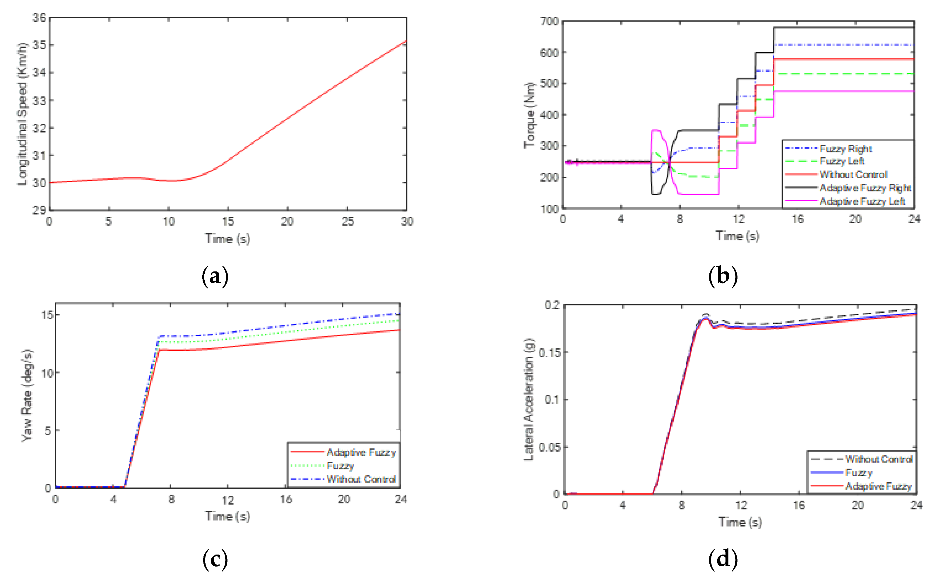
| Maximum yaw rate (deg/s) | 15.21 | 14.51 | 14.25 |
| Yaw rate deviation rate | 18% | 12% | 10% |
| Simulation Conditions | Without Control | Fuzzy Control | Adaptive Fuzzy Control |
|---|---|---|---|
| Maximum yaw rate (deg/s) | 5.53 | 4.88 | 4.45 |
| Maximum sideslip angle (deg) | 2.8 | 2.23 | 2.07 |
| Yaw rate deviation rate | 42% | 35% | 23% |
| Sideslip angle deviation rate | 58% | 25% | 16% |
| Simulation Conditions | Without Control | Fuzzy Control | Adaptive Fuzzy Control |
|---|---|---|---|
| Maximum yaw rate (deg/s) | −20.1 | 13.51 | 11.51 |
| Maximum sideslip angle (deg) | 10 | 4.1 | 2.6 |
| Yaw rate deviation rate | 83% | 31% | 12% |
| Sideslip angle deviation rate | 852% | 38% | 15% |
Publisher’s Note: MDPI stays neutral with regard to jurisdictional claims in published maps and institutional affiliations. |
© 2022 by the authors. Licensee MDPI, Basel, Switzerland. This article is an open access article distributed under the terms and conditions of the Creative Commons Attribution (CC BY) license (https://creativecommons.org/licenses/by/4.0/).
Share and Cite
Chen, H.; Wang, W.; Zhu, S.; Chen, S.; Gao, J.; Zhou, R.; Wei, W. Design of an Adaptive Distributed Drive Control Strategy for a Wheel-Side Rear-Drive Electric Bus. Electronics 2022, 11, 4223. https://doi.org/10.3390/electronics11244223
Chen H, Wang W, Zhu S, Chen S, Gao J, Zhou R, Wei W. Design of an Adaptive Distributed Drive Control Strategy for a Wheel-Side Rear-Drive Electric Bus. Electronics. 2022; 11(24):4223. https://doi.org/10.3390/electronics11244223
Chicago/Turabian StyleChen, Huipeng, Weiyang Wang, Shaopeng Zhu, Sen Chen, Jian Gao, Rougang Zhou, and Wei Wei. 2022. "Design of an Adaptive Distributed Drive Control Strategy for a Wheel-Side Rear-Drive Electric Bus" Electronics 11, no. 24: 4223. https://doi.org/10.3390/electronics11244223