Convolutional Network Research for Defect Identification of Productor Appearance Surface

Abstract

The accurate and rapid identification of surface defects is an important element of product appearance quality evaluation, and the application of deep learning for surface defect recognition is an ongoing hot topic. In this paper, a lightweight KD-EG-RepVGG network based on structural reparameterization is designed for the identification of surface defects on strip steel as an example. In order to improve the stability and accuracy in the recognition of strip steel surface defects, an efficient attention network was introduced into the network, and then a Gaussian error linear activation function was applied in order to prevent the neurons from being set to zero during neural network training, leaving neuron parameters without being updated. Finally, knowledge distillation is used to transfer the knowledge of the RepVGG-A0 network to give the lightweight model better accuracy and generalization capability. The outcomes of the experiments indicate that the model has a computational and parametric volume of 22.3 M and 0.14 M, respectively, in the inference phase, a defect recognition accuracy of 99.44% on the test set, and a single image detection speed of 2.4 ms, making it more suitable for deployment in real engineering environments.

1. Introduction

The detection of defects on a product’s surface is important underlying research in the area of intelligent production, and this paper investigates the detection of surface defects in strip steel during industrial production. The surface quality of strip steel is one of the most important indicators of strip steel quality and is linked to the quality of products downstream in areas such as automotive, household appliances and construction. The detection of surface defects in steel has therefore become an extremely significant task in the steel production sector.

The identification of productor surface defects is an important task for enterprise product lines. In the early days, the task was completed by human-eyes checking, and it was limited by the human limitations of the eyes. After the emergence of image processing technology, the task was then completed by the characteristics of the defect image. Zhou [1] et al. applied the SIFT algorithm to the identification of defects on the surface of medium-thick plates and achieved a good accuracy of 95% for defects that occur continuously. Hu [2] et al. extracted four visual features of the target image: geometry, shape, texture and greyscale and used a genetic algorithm to optimize a hybrid chromosome-based classification model for effective identification of image defects. However, the characteristics-based methods made it hard to check for tiny defects or other imperfections. In recent years, deep learning methods, such as the convolutional network, were proposed to be applied in certain fields.

Since the introduction of Alexnet [3] convolutional neural networks in 2012, they have demonstrated high efficiency and accuracy in object recognition. Convolutional neural networks have gradually become an important research direction in detection and recognition, and the accurate, fast and contact-free recognition techniques are continuously investigated. Manzo [4] et al. used some pre-trained convolutional neural networks to detect the COVID-19 disease in CT images and gained an accuracy of 96.5%. Jiang [5] et al. used an improved VGG network to identify rice and wheat leaf disease simultaneously. Tao [6] et al. accurately identified smaller flames using an improved GoogLeNet network. As a new research hotspot, deep convolutional neural networks have been used in a wide range of industries.

Convolutional neural networks have been extensively applied to product surface defect recognition. Vonnocc [7] et al. used traditional machine learning methods and deep learning methods to classify surface defects in hot rolled strip steel, and they found that the deep learning approach worked better. Konovalenko [8] et al. detected surface defects in strip steel based on the ResNet50 framework, with a precision of 96.91% in recognition. Xiang [9] et al. used a small sample dataset to achieve an accurate recognition rate of 97.8% on an improved VGG-19 network. Feng [10] et al. added FcaNet and CMAM modules based on Resnet, achieving an accuracy of 94.11% for the defect identification in hot-rolled strip steel. Tang [11] et al. used multi-scale maximum pooling and an attention mechanism to detect surface defects, where the classification accuracy rate reaches 94.73%. Xing [12] proposes a convolutional classification model with symmetric structure to achieve accurate recognition of surface defects. These studies have focused on accuracy design, ignoring the computational volume, complexity and real-time requirements of the models in real-world applications. Wang [13] et al. designed the VGG-ADB model for defect recognition, which achieved 99.63% classification accuracy and 333 frame/s inference speed. The VGG-ADB model considered the inference speed of the network, but the model was ignored for the parametric design, where the model size reached 72.15 M. This constrained the application of the model on edge devices. In actual production, not only does the network require extremely high detection accuracy, but it also has high requirements for model size, detection speed and real-time detection.

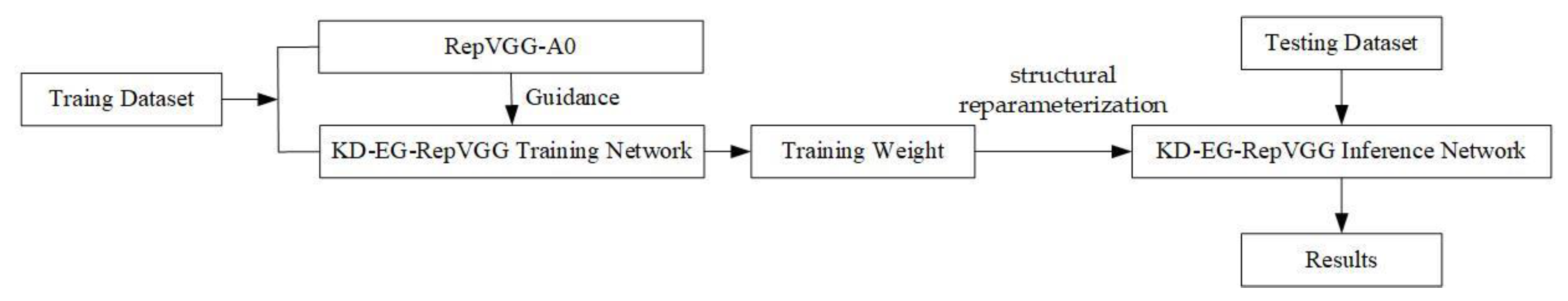
The KD-EG-RepVGG surface defect detection algorithm is designed using structural reparameterization, GELU, ECA networks and knowledge distillation for the task requirement of surface defects identification. Through experimental comparative analysis, the KD-EG-RepVGG network is characterized by a low number of parameters, low computational effort, high speed and high accuracy. The general idea of the method in the paper is illustrated in Figure 1. The teacher network RepVGG-A0 guides the KD-EG-RepVGG network training. The structural re-parameterization technique loads the training weights into the KD-EG-RepVGG inference network to finally obtain the prediction results.

This paper is structured as follows. Section 2 describes in detail the KD-EG-RepVGG network framework. Section 3 verifies the validity of the network from several perspectives, whereas Section 4 is the conclusion of the paper.

2. The KD-EG-RepVGG Network

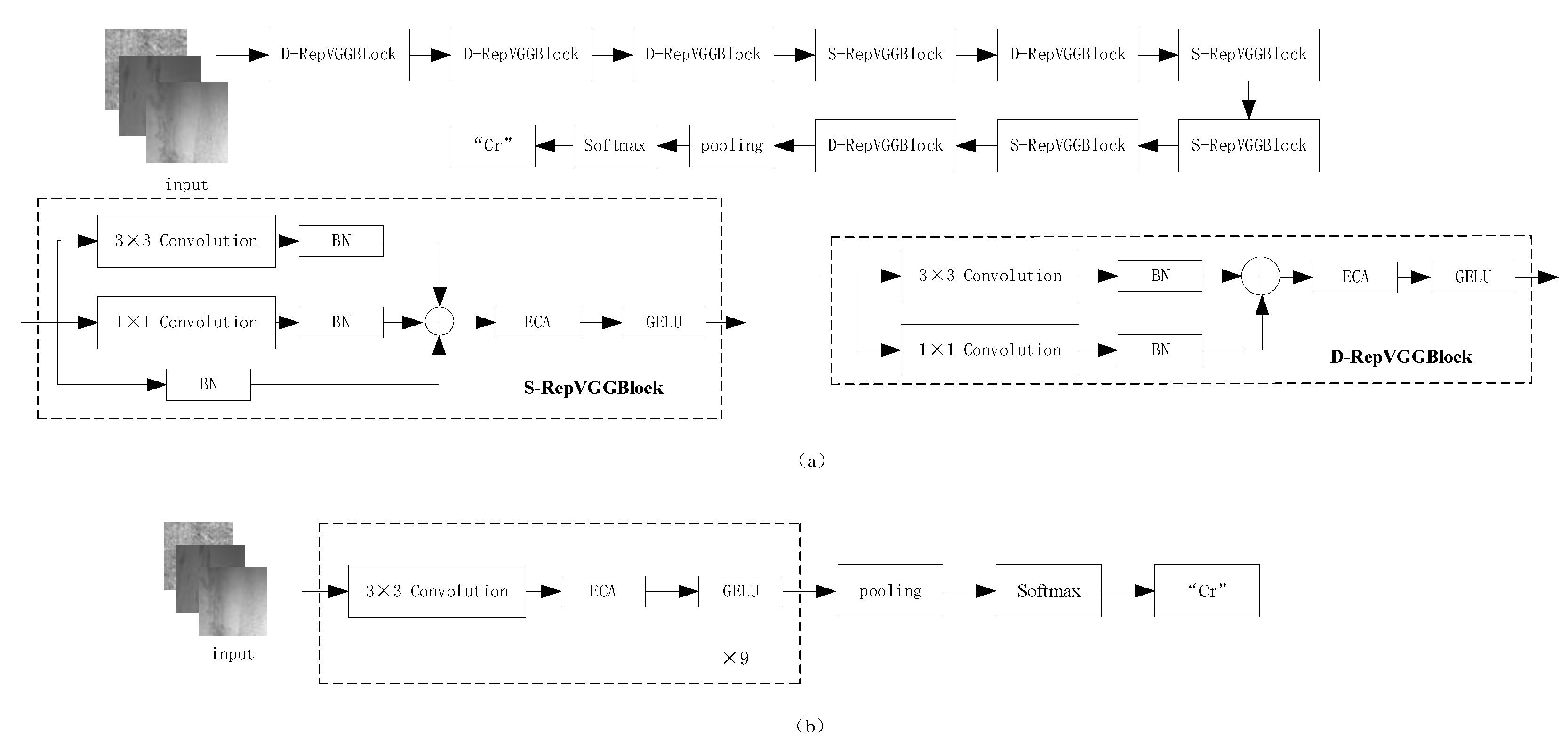
The EG-RepVGG network is based on structural reparameterization, incorporating a lightweight attention network while using GELU as the activation function in the improved network, stacking the S-RepVGG block module and D-RepVGG block module based on RepVGGBlock. The model is structured as shown in Figure 2. The main function of the D-RepVGG block module is to extract features and adjust the space size and channel number of the feature map, whereas the main purpose of the S-RepVGG block is feature extraction. The S-RepVGG block has an additional directly connected structure compared to the D-RepVGG block, which mimics the residual connection in ResNet [14] and improves the model’s ability to extract features. The output of D-RepVGG Block5 is made up of global average pooling and then a softmax classifier is appended. The global average pooling layer is used to downsample the output spatial resolution of the feature map to 1 × 1. The softmax layer is used to output the predicted categories. They together form the classification layer. With the aim of further improving the accuracy and generalization performance of the model, the RepVGG-A0 as a teacher model is used to guide the training of EG RepVGG model using knowledge distillation technology. The final result is a lightweight, fast and highly accurate strip steel surface defect recognition model, the KD-EG RepVGG model. The detailed structural information of the KD-EG-RepVGG model is shown in

Table 1. KD-EG-RepVGG Network Structure Details.

Layers	Output Size	Output Channel	Train Parameters	Inference Parameters
input	200 × 200	3
D-RepVGGBlock1	100 × 100	9	309	252
D-RepVGGBlock2	50 × 50	9	849	738
D-RepVGGBlock3	25 × 25	19	1789	1558
S-RepVGGBlock1	25 × 25	19	3727	3268
D-RepVGGBlock4	13 × 13	38	7375	6536
S-RepVGGBlock2	13 × 13	38	14,671	13,034
S-RepVGGBlock3	13 × 13	38	14,671	13,034
S-RepVGGBlock4	13 × 13	38	14,671	13,034
D-RepVGGBlock5	7 × 7	256	98,307	87,808
Classification	1 × 1	6	1542	1542

.

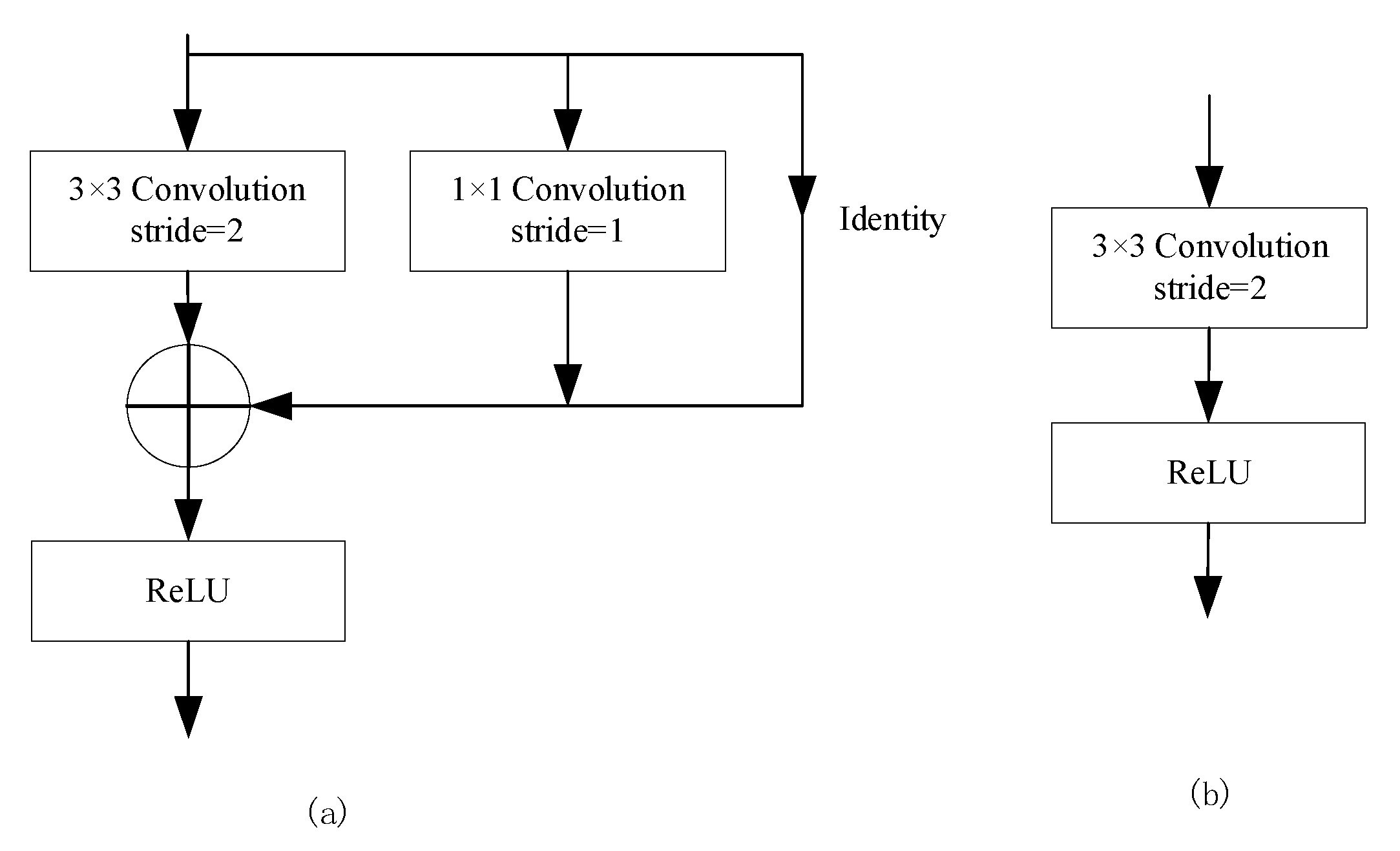
2.1. Structural Re-Parameterisation

The structural reparameterization was first proposed in RepVGG networks by Ding XiaoHan [15] et al. The inference network is decoupled from the training network using structural reparameterization techniques. Decoupling the training network and inference network by using structure re-parameterization can not only obtain the full advantage of feature extraction brought by multi branch network training, but also obtain the high speed and low memory consumption of a single path model in inference deployment. The core component of the RepVGG network is the RepVGG Block. Its structure is shown in Figure 3.

The structure of the network under training is illustrated in Figure 3a. In the training phase, the RepVGG Block consists mainly of 3 × 3 convolutional kernels, 1 × 1 convolutional kernels and Identity branches. By adding Identities branches and 1 × 1 convolutional branches in parallel, information at different scales of the image can be extracted and fused, increasing the representational power of the model.

In the inference stage, the 1 × 1 convolution and Identity branch from the training are fused into the 3 × 3 convolution, and the inference structure is shown in Figure 3b. RepVGG Block takes the training network and re-parameterizes it structurally, turning the network into a single linear structure consisting mainly of 3 × 3 convolutions without any branches. The inference structure both gains the parameter weights obtained from multi-branch training and allows the use of the single linear structure to speed up the inference of the model during the deployment inference phase. At the same time, deep optimization of the 3 × 3 convolution based on NVIDIA cuDNN’s computational library accelerates the model’s detection speed in the inference phase.

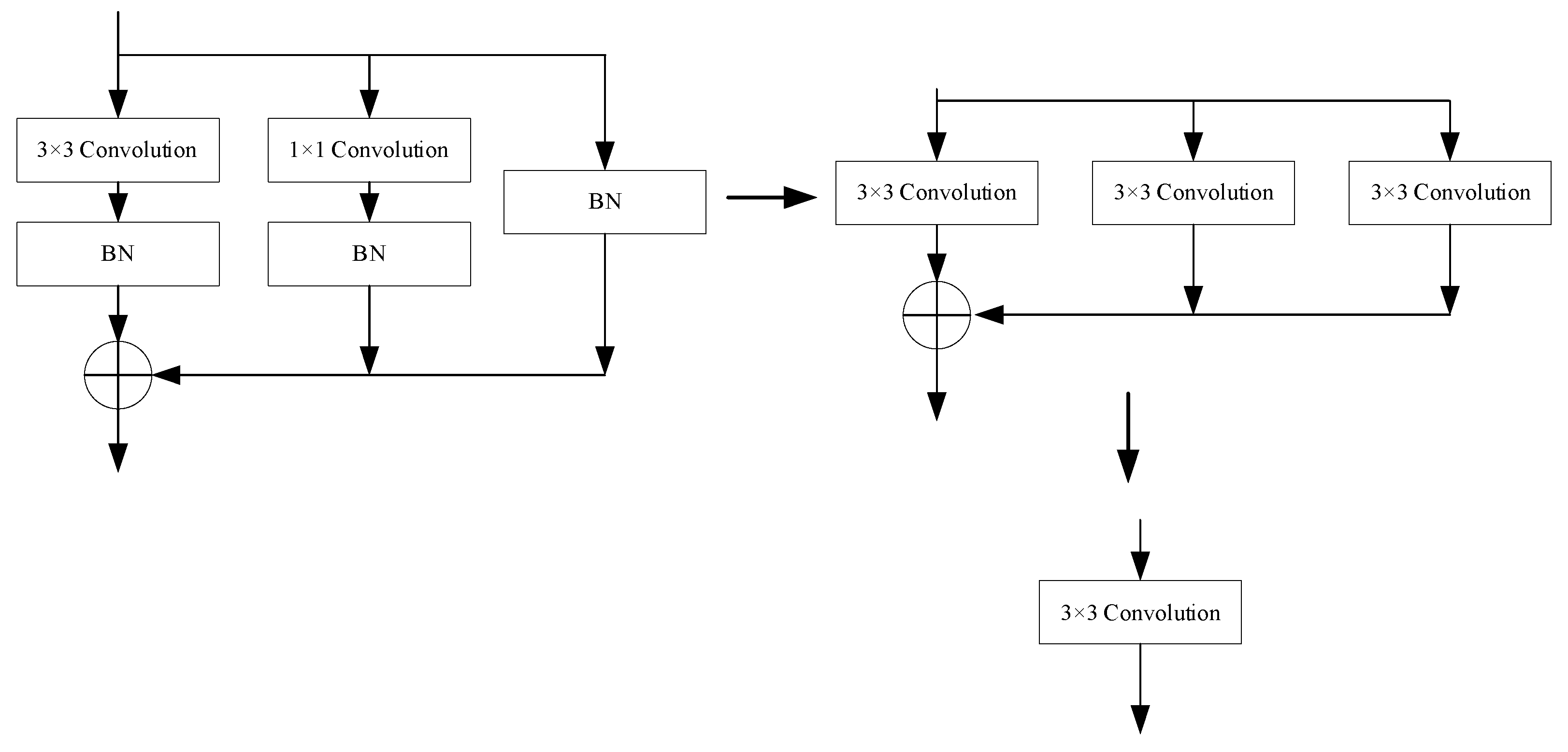
The structural reparameterization in the inference phase mainly consists of the fusion of the convolution kernel and the Batch Normalization (BN) layer [16], the integration of 1 × 1 convolution into 3 × 3 convolution and the integration of Identity branches into 3 × 3 convolution. The formula for the fusion of the convolution and BN layers in the model is as follows:

$$BN\left(x\right)=\frac{x-\mu }{\sqrt{{\sigma }^2+\epsilon }}\gamma +\beta$$

(1)

where $\mu$ denotes the mean of the BN layer and ${\sigma }^2$ denotes the BN layer variance; $\mu$ and ${\sigma }^2$ are obtained statistically in the training dataset; $ϵ$ is a constant to prevent the denominator from being zero; $\gamma$ is the scale factor of the BN layer; $\beta$ is the offset of the BN layer and the values of both $\gamma$ and $\beta$ are obtained in the training.

For convolution, the formula is as it is in (2):

$$Conv\left(x\right)=Wx+b$$

(2)

where $x$ and $Conv\left(x\right)$ are the input and output of the convolution; $W$ denotes the matrix weight of the convolution calculation; and $b$ is the bias of the convolution layer calculation.

The input to the BN layer is the output of the convolution into it. This is equivalent to taking Equation (2) and bringing it into Equation (1), resulting in a calculation such as Equation (3):

$$BN\left(x\right)=\frac{\left(Wx+b\right)}{\sqrt{{\sigma }^2+\epsilon }}\gamma +\beta$$

(3)

The following can be obtained by sorting and simplifying:

$$BN\left(x\right)=\frac{\gamma }{\sqrt{{\sigma }^2+\epsilon }}Wx+\left( \frac{\gamma \left(b-\mu \right)}{\sqrt{{\sigma }^2+\epsilon }}+\beta \right)$$

(4)

From the calculation results, we can obtain a new convolution by incorporating the weight information calculated by Batch Normalization layer into the convolution layer, where the convolution weight is $\frac{\gamma }{\sqrt{{\sigma }^2+\epsilon }}W$, and the bias of the convolution is$\frac{\gamma \left(b-\mu \right)}{\sqrt{{\sigma }^2+\epsilon }}+\beta$.

For the Identity branch in the RepVGG Block, a 1 × 1 convolution kernel with a weight of 1 is used to construct a 1×1 convolution, and then a 3 × 3 convolution kernel is set to perform identity mapping on the input features. Keep the output of the Identity layer unchanged before and after the transformation. For a 1 × 1 convolution branch, a complementary zero operation is performed around the 1 × 1 convolution kernel so that it becomes a 3 × 3 convolution. At this point, both the 1 × 1 convolution and Identity are converted into a 3 × 3 convolution, and based on the additivity of the convolution operation, the three branches can then be incorporated into a single 3 × 3 convolution. The process is shown in Figure 4.

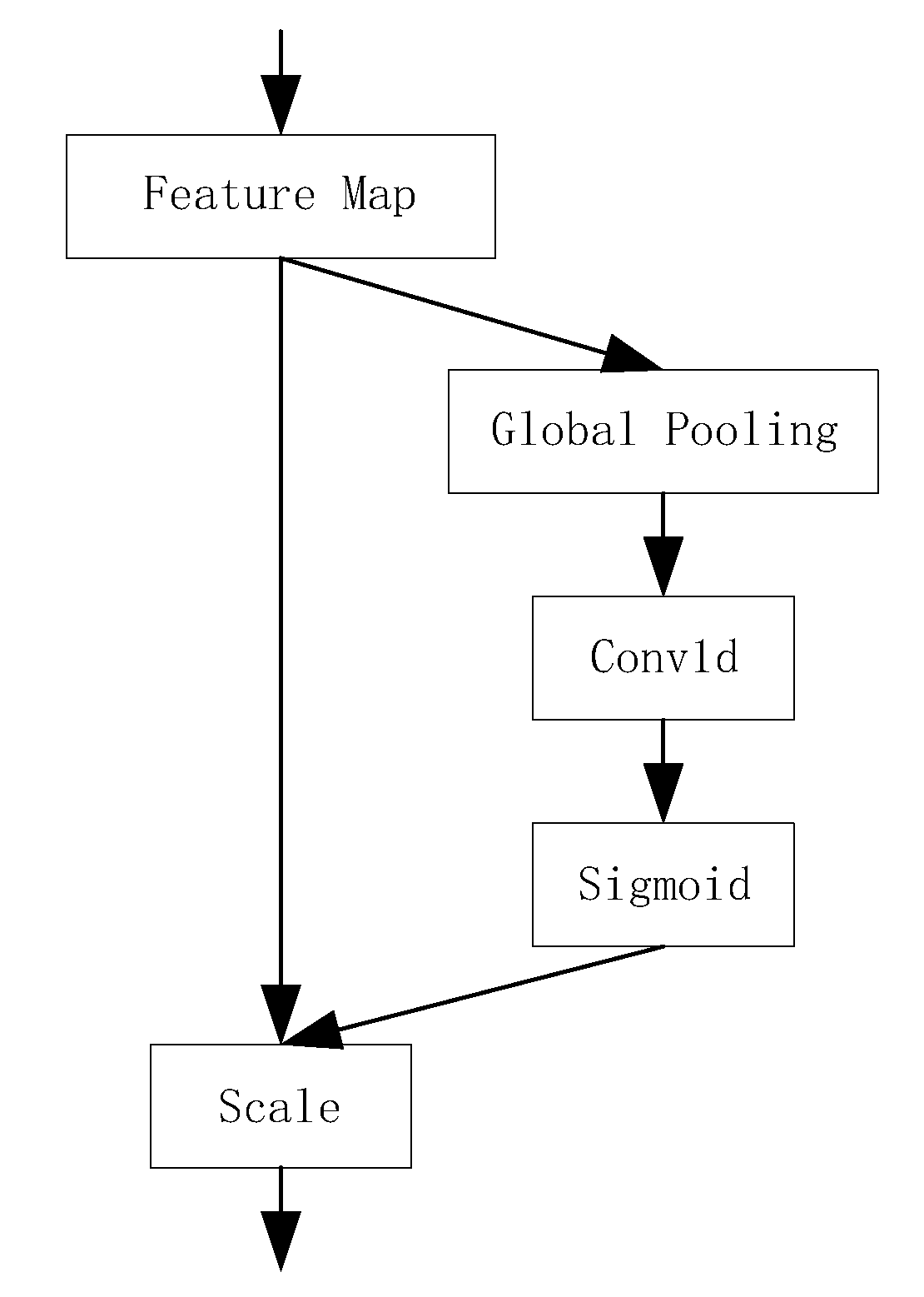
2.2. Efficient Channel Attention Network

The Efficient Channel Attention network [17] was added to the RepVGG Block to form the E-RepVGG network. The feature information can be obtained efficiently and without increasing the number of parameters of the model at the same time. The structure of ECA is shown in Figure 5. The feature map $x\in {ℝ}^{L\times S\times T}$ output from the convolution is pooled and globally averaged (Global Pooling) over the spatial dimension to output a feature vector $y$ of size $1\times 1\times T$, as is shown in Equation (5):

$$y=\frac{1}{WH}{\displaystyle \sum }_{i=1,j=1}^{W,H}{x}_{i,j}$$

(5)

where $L$and $S$ are the width and height of the feature map, respectively; and $T$ is the number of channels in the feature map. Channel weighting coefficient obtained after the ECA network can be calculated by the following equation:

$$\mathsf{\Psi }=sigmod\left(\mathsf{\Omega }y\right)$$

(6)

where $sigmoid$ is the sigmoid activation function; Ψ is the weight of the ECA network on the channel; and $\Omega$ is the parameter matrix for calculating the channel attention in ECA networks. The mathematical model is represented as follows:

$$\Omega =\left[\begin{array}{cc}\begin{array}{ccc}{\omega }^{1,1}& \cdots & {\omega }^{1,k}\end{array}& \begin{array}{cc}\cdots & 0\end{array}\\ \begin{array}{ccc}0& {\omega }^{2,2}& \cdots \\ ⋮& ⋮& ⋮\\ 0& \cdots & 0\end{array}& \begin{array}{cc}\cdots & 0\\ ⋮& ⋮\\ \cdots & {\omega }^{T,T}\end{array}\end{array}\right]$$

(7)

It is clear from $\Omega$ that the weight value of $\mathsf{\Psi }$is determined only by the $k$ channels in the immediate vicinity of $y$. This can be expressed as a 1-dimensional convolution ($Conv1d)$with a kernel of size$k$. Bringing in the simplification yields:

$$\mathsf{\Psi }=sigmoid\left(Conv1d\left(y\right)\right)$$

(8)

where$Conv1d$ denotes a 1-dimensional convolution of convolution kernel size k. In this paper, considering the model parameters and inference speed, the size of all 1-dimensional convolution kernels is set to 3.

The weight coefficients of each channel calculated by the efficient attention network are multiplied by the channel weights of the input feature map $x\in {ℝ}^{L\times S\times T}$ to obtain the output:

$$\tilde{x}=\mathsf{\Psi }x$$

(9)

where $\tilde{x}\in {ℝ}^{L\times S\times T}$ is the output of the ECA network.

2.3. Gaussian Linear Units

The rectified linear units (ReLU) activation function is used in the RepVGG Block, which effectively solved the problem of disappearing or exploding gradients as the neural network deepens. However, the ReLU activation function also has some problems. When the input is less than zero, the ReLU output will be directly zeroed, and the neuron will be permanently zeroed, which is detrimental to the convergence of the network model and feature extraction. Therefore, Gaussian Error Linear Units [18] (GELU) are selected as the activation function in this paper to form the EG-RepVGG network. The GELU activation function is applied as a non-linear unit after the ECA network. The GELU activation function is differentiable at the origin, and the idea of stochastic regularity is introduced into the function. The activation operation will establish a stochastic connection between the input and output, effectively avoiding the situation where the neurons are set to zero and enhancing the learning speed and stability of the network.

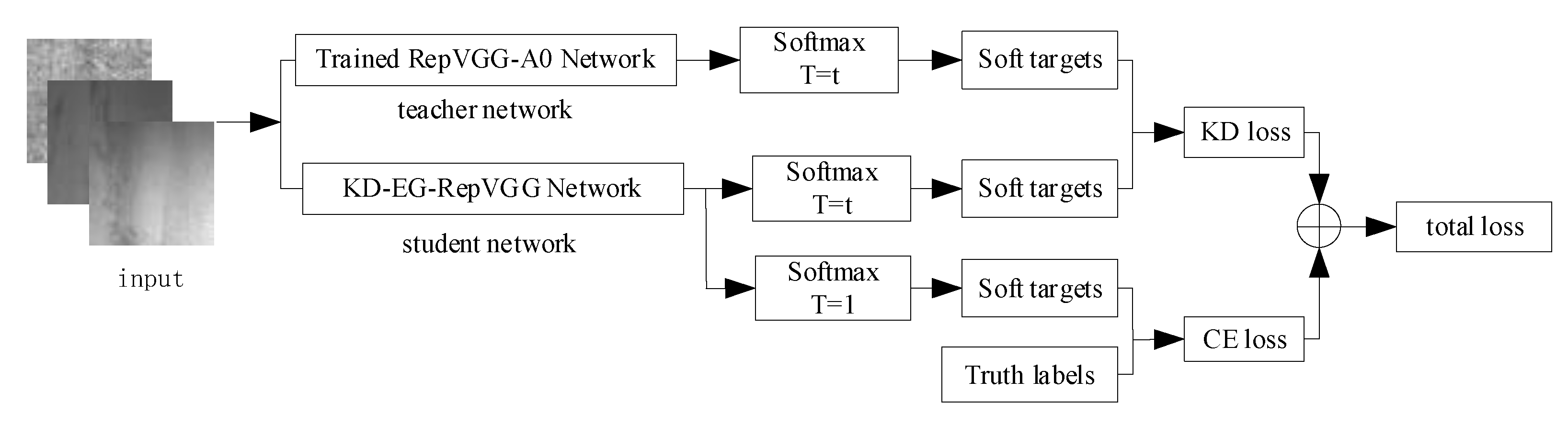
2.4. Knowledge Distillation

The knowledge distillation is a novel technique for model compression proposed by Geoffrey Hinton [19] et al. A complex, highly generalizable large model is used to guide the training of a lightweight small model, allowing the small model to achieve the same accuracy as the large model at a smaller cost. At the heart of the knowledge distillation network is the fact that the different classes of confidence in the output of the teacher network define a rich similarity structure at the data level and can provide more inter- class knowledge for small networks to guide the training of small networks. The characteristic distillation is calculated by:

$$q_i=\frac{e^{\frac{z_i}{T}}}{{{\displaystyle \sum }}_i{e}^{\frac{Z_i}{T}}}$$

(10)

The activation operation will establish a stochastic connection between the input and output, effectively avoiding the situation where the neurons are set to zero and enhancing the learning speed and stability of the network. The hyperparameter $T$ softens the output categories of the large and small networks to find the distillation loss of the two networks’ outputs and the direct training output loss of the small network. The two losses are weighted and summed to obtain the training losses of the networks. The entire knowledge distillation network training process is shown in Figure 6. In this paper, the KD-EG-RepVGG network was obtained by using RepVGG-A0 as the teacher network and instructing the training of the EG-RepVGG network.

The loss function used in the training phase is the $KL$ scatter loss and the cross-entropy loss weighted sum is used as the final loss for training and the loss formula is as in (11)

$$Loss=\alpha ·L_{kd}\left(q\left(u,T\right),q\left(z,T\right)\right)+\left(1-\alpha \right)·L_s\left(y,q\left(z,1\right)\right)$$

(11)

$$L_{kd}={\displaystyle \sum }_{i=1}^N{q}_i\left(u_i,T\right)\log q_i\left(u_i,T\right)-{\displaystyle \sum }_{i=1}^N{q}_i\left(u_i,T\right)\log q_i\left(z_i,T\right)$$

(12)

$$L_s=-{\displaystyle \sum }_{i=1}^N{y}_i\log q_i\left(z_i,1\right)$$

(13)

where $N$ is the number of categories of defects; $q\left(u,T\right)$ represents the information about the features of the teacher network after the distillation temperature; $q\left(z,T\right)$ represents the information about the features of the student network after the distillation temperature; $L_{kd}$ is the scatter loss, an asymmetry measure of the difference between the probability distributions of $q\left(u,T\right)$ and $q\left(z,T\right)$. This is shown in Equation (12). $L_s$ is the cross-entropy loss, which indicates how close the predicted output value is to the true sample label, as shown in Equation (13). In this paper, the distillation temperature$T=7$. α is the default value, which in this paper is 0.3 by default.

3. Experiments and Analysis of Results

3.1. Experimental Paltform

The experimental platform includes: an Intel Core i7-11700F processor, a Nvidia GeForce RTX3060 12 GB graphics card, 32 GB memory; the software is Windows 10 operating system, python 3.8; and the deep learning framework used is pytorch.

3.2. Experimental Data Sets

This paper uses the NEU-CLS dataset [20] of strip surface defects produced and published by Northeastern University for experiments. As shown in Figure 7, the surface defects of the data strip are divided into six categories: Crack (Cr), Inclusion (In), Patch (Pa), Pitted Surface (Ps), Rolled-in Scale (Rs) and Scratch (Sc).

Table 2. Information on the data set.

Defect Category	Pixel	Channel	Amount
Crack	200 × 200	1	300
Inclusion	200 × 200	1	300
Patch	200 × 200	1	300
Pitted Surface	200 × 200	1	300
Rolled-in Scale	200 × 200	1	300
Scratch	200 × 200	1	300

shows the details of each defective picture. The total 1800 images in the table are divided into training set, validation set and test set at the ratio of 8:1:1. The training set has 1440 images, and the validation set and test set have 180 images each.

3.3. Experimental Results and Analysis

To analyze and measure the comprehensive performance of the network model in the identification task of strip surface defects, the accuracy, the Matthew’s correlation coefficient, FPS, single picture detection time, model parameters and FLOPs were used to evaluate the model.

The accuracy (ACC) rate is the proportion of correctly classified samples to all samples. The higher the accuracy rate, the better the classification effect of the model, and the formula is shown in 14. The Matthews correlation coefficient (MCC) is used to calculate the correlation between the actual classification and the predicted classification, and it is a balanced evaluation index. The value range of MCC is between −1 and 1. When the value of MCC is closer to 1, the result predicted by the classifier is more reliable.

$$TP=\frac{TP+TN}{ALL}$$

(14)

where $TP$ is the number of samples correctly predicted by positive samples, $TN$ is the number of negative samples correctly predicted, and$ALL$ is the number of all samples.

3.3.1. Ablation Experiments

The comprehensive performance of KD-EG-RepVGG was evaluated on the NEU-CLS test set and the results are shown in

Table 3. Comparative experimental results of distillation.

Model	Accuracy	MCC	Time	Params	FLOPs
RepVGG-A0	98.83%	97.91%	5.1 ms	7.04 M	1.36 G
EG-RepVGG	97.22%	96.39%	2.4 ms	0.14 M	0.03 G
KD-EG-RepVGG	99.44%	99.02%	2.4 ms	0.14 M	0.03 G

. The super parameter setting in the teacher network RepVGG-A0 is also applied in the KD-EG-RepVGG network. The network is trained using the stochastic gradient decent (SGD) optimizer with a momentum coefficient of 0.9 and weight decay of 0.0001. The learning rate is set to 0.1. Batch Size and epochs are kept at 64 for 100, respectively.

The comparison revealed that the lightweight model KD-EG-RepVGG after knowledge distillation had an accuracy improvement of greater than two percentage points over the EG-RepVGG model. Furthermore, the accuracy of the lightweight KD-EG-RepVGG network after knowledge distillation was improved by 0.6 percentage points over the teacher network RepVGG-A0. The Matthew’s correlation coefficient of KD-EG-RepVGG on the test set is 99.02%, which further proves that the model is very accurate in identifying the surface defects of the strip. Figure 8 shows the validation accuracy and loss curve of the network. From the curve change trend, we can find that the KD-EG-RepVGG network converges faster and the model accuracy is higher. The aim of transferring the knowledge of large models to small networks and improving the accuracy and generalizability of the networks is achieved.

Furthermore, to analyze more clearly the capabilities of the model, we calculated the confusion matrix of the model on the test set and the results are shown in Figure 9. From the confusion matrix, it can be obtained that the model had a high recognition rate of defects. The recall rate was calculated according to the confusion matrix, and it was found that only the “In” defect was 97.30%, and the other defects were 100%. The precision was calculated, and it was found that only the “Sc” defect is 97.13%, and the other defects were 100%.

3.3.2. Comparative Experimental Analyses

The KD-EG-RepVGG algorithm was compared with the current mainstream advanced algorithms on the same test set. To demonstrate the validity of the models, the KD-EG-RepVGG is compared with ResNet50, VGG16, ShuffleNetV2 and MobileNetV2 models in the same software and hardware environment. The accuracy, FPS, single picture detection time, calculation amount, parameter amount and other detection indicators of various algorithms are compared and analyzed. The results of the experiment are recorded in

Table 4. Comparison of test results for different algorithms.

Model	Accuracy (%)	Time (ms)	FPS (Frame/s)	Params (M)	FLOPs (G)
ResNet50	96.67	6.8	146.9	24.56	4.12
VGG16	95.87	6	143.3	138.3	15.61
ShuffleNetV2	97.25	6	167.4	2.26	0.15
MobileNetV2	96.94	6.2	161.4	3.4	0.33
KD-EG-RepVGG	99.44	2.4	408	0.14	0.03

.

In comparison, the KD-EG-RepVGG network achieves better classification accuracies than the larger parametric models, VGG16 and ResNet50, outperforming ResNet50 by almost three percentage points. Compared with the lightweight networks shuffleNetV2 and MobileNetV2, the KD-EG-RepVGG network has achieved great advantages in reasoning speed, parameter amount and computation amount. The KD-EG-RepVGG network is more suitable for industrial applications because it achieves an increase in detection efficiency, detection accuracy and detection speed while consuming very little memory and few computing resources.

3.4. Model Visualisation

The features of the middle layer of the convolutional neural network model are visualized in order to gain a clearer understanding of the features learned with the convolutional neural network [21]. A random selection of defective images is fed into the KD-EG-RepVGG inference network, which visualizes the convolutional layers in the network. The visualization results are shown in Figure 10. In the KD-EG-RepVGG network, the shallow convolutional network retains the image information relatively intact, with the main detection being contour information. The deeper convolutional layers focus more on the location features of the target and some abstract information. From the visualization results, it can be observed that important regional features in the image are encoded into the network, indicating that the network is effective for feature learning.

The Gradient Weighted Class Activation Mapping algorithm [22] (Grad-CAM) is used to fully demonstrate the ability of the KD-EG-RepVGG network to extract defective features. A heat map was used to show the activated regions in the images, which is more consistent with human vision properties. This is more in line with human visual properties. The final layer of the KD-EG-RepVGG network was chosen for visual representation in this paper. This is because it is a generalized representation of the feature extraction from the previous layer of the network. Images of six types of defects were randomly selected for visualization with darker colors indicating that the network is paying more attention to the point. This is shown in Figure 11.

As can be viewed in Figure 11, the KD-EG-RepVGG’s extraction of defect features is focused on salient feature points, and the KD-EG-RepVGG network demonstrates high efficiency by focusing on only one feature point for the same feature in the case of impurities, spot cracks and pockmark defects. The KD-EG-RepVGG also has the ability to recognize features from multiple angles. The features of cracks at different locations and angles can be fully extracted, demonstrating a strong extraction capability.

4. Conclusions

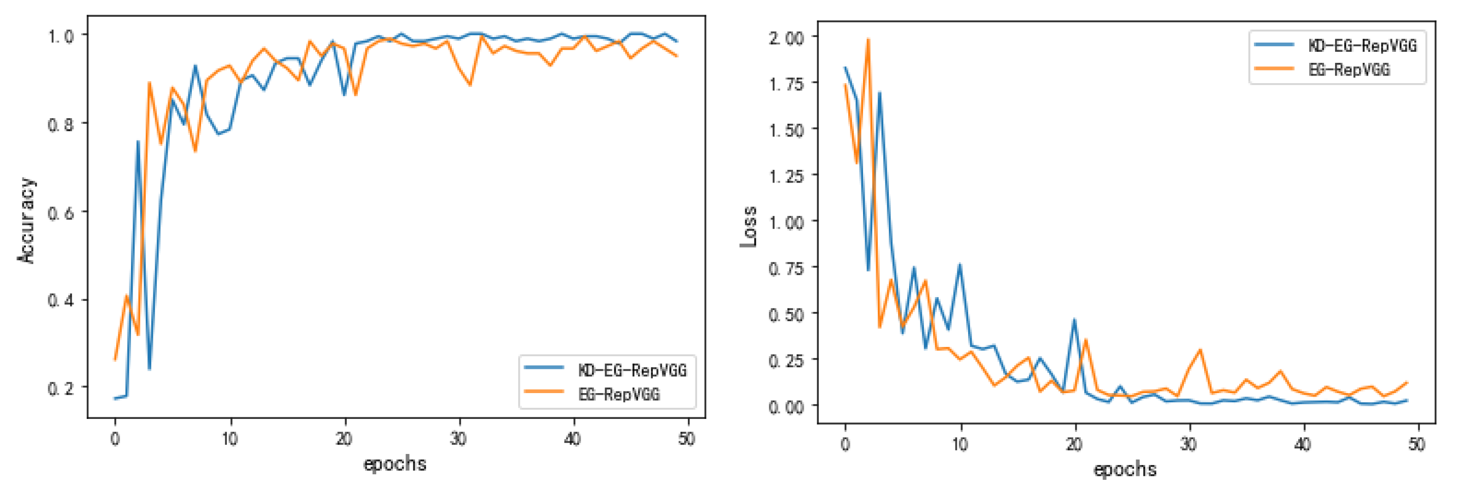
Aiming at the requirement of strip surface defect detection in actual production, a strip defect recognition method based on a structural re-parameterized KD-EG-RepVGG network is proposed. In RepVGG Block, the ECA network and GELU activation functions are added. Among them, the ECA network improves the accuracy of the KD-EG-RepVGG network while increasing the convergence speed of KD-EG-RepVGG. The GELU activation function avoids neuron necrosis caused by zeroing. Through knowledge distillation technology, the KD-EG-RepVGG model obtains the knowledge of RepVGG-A0, which improves the accuracy and robustness of the model. Through ablation experiments and comparative analysis with other models, it can be seen that the lightweight KD-EG RepVGG network takes up very little memory resources and computing resources without affecting the accuracy, and has a faster detection speed. It is more suitable for deployment and uses in real production.

The future work involves many directions. Firstly, the research in this paper will be used as a basis to study the accurate localization of defects and to analyze the size of defects accurately. Then, the model will be deployed on edge equipment and applied in the production environment within plants.

References

1. Peng, Z.; Ke, X.; Chaolin, Y. Surface defect recognition for moderately thick plates based on a SIFT operator. J. Tsinghua Univ. (Sci. Technol.) 2018, 58, 881–887. [Google Scholar]
2. Hu, H.; Liu, Y.; Liu, M.; Nie, L. Surface defect classification in large-scale strip steel image collection via hybrid chromosome genetic algorithm. Neurocomputing 2016, 181, 86–95. [Google Scholar] [CrossRef]
3. Krizhevsky, A.; Sutskever, I.; Hinton, G.E. Imagenet classification with deep convolutional neural networks. Adv. Neural Inf. Process. Syst. 2012, 25, 1097–1105. [Google Scholar] [CrossRef] [Green Version]
4. Manzo, M.; Pellino, S. Fighting Together against the Pandemic: Learning Multiple Models on Tomography Images for COVID-19 Diagnosis. AI 2021, 2, 16. [Google Scholar] [CrossRef]
5. Jiang, Z.; Dong, Z.; Jiang, W.; Yang, Y. Recognition of rice leaf diseases and wheat leaf diseases based on multi-task deep transfer learning. Comput. Electron. Agric. 2021, 186, 106184. [Google Scholar] [CrossRef]
6. Tao, L.; Wang, L.; Shen, X.; Liu, C. Research of Fire Identification Method Based on Convolutional Neural Network. In Proceedings of the 2022 7th International Conference on Intelligent Computing and Signal Processing (ICSP), Xi’an, China, 15–17 April 2022; pp. 1656–1659. [Google Scholar]
7. Vannocci, M.; Ritacco, A.; Castellano, A.; Galli, F.; Vannucci, M.; Iannino, V.; Colla, V. Flatness Defect Detection and Classification in Hot Rolled Steel Strips Using Convolutional Neural Networks. In Proceedings of the 15th International Work-Conference on Artificial Neural Networks (IWANN), Granada, Spain, 12–14 June 2019; pp. 220–234. [Google Scholar]
8. Konovalenko, I.; Maruschak, P.; Brezinova, J.; Vinas, J.; Brezina, J. Steel Surface Defect Classification Using Deep Residual Neural Network. Metals 2020, 10, 846. [Google Scholar] [CrossRef]
9. Wan, X.; Zhang, X.; Liu, L. An improved VGG19 transfer learning strip steel surface defect recognition deep neural network based on few samples and imbalanced datasets. Appl. Sci. 2021, 11, 2606. [Google Scholar] [CrossRef]
10. Feng, X.; Gao, X.; Luo, L. A ResNet50-Based Method for Classifying Surface Defects in Hot-Rolled Strip Steel. Mathematics 2021, 9, 2359. [Google Scholar] [CrossRef]
11. Tang, M.; Li, Y.; Yao, W.; Hou, L.; Sun, Q.; Chen, J. A strip steel surface defect detection method based on attention mechanism and multi-scale maxpooling. Meas. Sci. Technol. 2021, 32, 115401. [Google Scholar] [CrossRef]
12. Xing, J.; Jia, M. A convolutional neural network-based method for workpiece surface defect detection. Measurement 2021, 176, 109185. [Google Scholar] [CrossRef]
13. Wang, W.; Lu, K.; Wu, Z.; Long, H.; Zhang, J.; Chen, P.; Wang, B. Surface Defects Classification of Hot Rolled Strip Based on Improved Convolutional Neural Network. ISIJ Int. 2021, 61, 1579–1583. [Google Scholar] [CrossRef]
14. He, K.M.; Zhang, X.Y.; Ren, S.Q.; Sun, J.; IEEE. Deep Residual Learning for Image Recognition. In Proceedings of the 2016 IEEE Conference on Computer Vision and Pattern Recognition (CVPR), Las Vegas, NV, USA, 27–30 June 2016; pp. 770–778.
15. Ding, X.H.; Zhang, X.Y.; Ma, N.N.; Han, J.G.; Ding, G.G.; Sun, J.; Ieee Comp, S.O.C. RepVGG: Making VGG-style ConvNets Great Again. In Proceedings of the IEEE/CVF Conference on Computer Vision and Pattern Recognition (CVPR), Electr Network, 19–25 June 2021; pp. 13728–13737. [Google Scholar]
16. Ioffe, S.; Szegedy, C. Batch Normalization: Accelerating Deep Network Training by Reducing Internal Covariate Shift. In Proceedings of the 32nd International Conference on Machine Learning, Lille, France, 7–9 July 2015; pp. 448–456. [Google Scholar]
17. Wang, Q.; Wu, B.; Zhu, P.; Li, P.; Zuo, W.; Hu, Q. ECA-Net: Efficient Channel Attention for Deep Convolutional Neural Networks. In Proceedings of the 2020 IEEE/CVF Conference on Computer Vision and Pattern Recognition (CVPR), Seattle, WA, USA, 13–19 June 2020; pp. 11531–11539. [Google Scholar]
18. Hendrycks, D.; Gimpel, K. Gaussian error linear units (gelus). arXiv 2016, arXiv:1606.08415. [Google Scholar]
19. Hinton, G.; Vinyals, O.; Dean, J. Distilling the knowledge in a neural network. arXiv 2015, arXiv:1503.02531. [Google Scholar]
20. Bao, Y.Q.; Song, K.C.; Liu, J.; Wang, Y.Y.; Yan, Y.H.; Yu, H.; Li, X.J. Triplet-Graph Reasoning Network for Few-Shot Metal Generic Surface Defect Segmentation. Ieee Trans. Instrum. Meas. 2021, 70, 1–11. [Google Scholar] [CrossRef]
21. Wagner, J.; Kohler, J.M.; Gindele, T.; Hetzel, L.; Wiedemer, J.T.; Behnke, S.; Soc, I.C. Interpretable and Fine-Grained Visual Explanations for Convolutional Neural Networks. In Proceedings of the 32nd IEEE/CVF Conference on Computer Vision and Pattern Recognition (CVPR), Long Beach, CA, USA, 16–20 June 2019; pp. 9089–9099. [Google Scholar]
22. Selvaraju, R.R.; Cogswell, M.; Das, A.; Vedantam, R.; Parikh, D.; Batra, D. Grad-CAM: Visual Explanations from Deep Networks via Gradient-Based Localization. Int. J. Comput. Vis. 2020, 128, 336–359. [Google Scholar] [CrossRef]
Figure 1. General diagram of defect identification process.
Electronics 11 04218 g001
Figure 2. KD-EG-RepVGG Network. (a) KD-EG-RepVGG Training Network. (b) KD-EG-RepVGG Inference Network.
Electronics 11 04218 g002
Figure 3. RepVGG Block structure diagram. (a) RepVGG Block training. (b) RepVGG Block inference.
Electronics 11 04218 g003
Figure 4. RepVGG Block branched fusion process.
Electronics 11 04218 g004
Figure 5. ECA network structure diagram.
Electronics 11 04218 g005
Figure 6. Knowledge distillation procedure.
Electronics 11 04218 g006
Figure 7. Example of defective image and corresponding label. (a) Crack, (b) Inclusion, (c) Patch, (d) Pitted Surface, (e) Rolled-in Scale, (f) Scratch.
Electronics 11 04218 g007
Figure 8. Validation set accuracy curves and loss curves.
Electronics 11 04218 g008
Figure 9. Confusion matrix.
Electronics 11 04218 g009
Figure 10. Convolutional layer visualization for RepVGG networks.
Electronics 11 04218 g010
Figure 11. KD-EG-RepVGG network heat map.
Electronics 11 04218 g011