Analysis of Impulse Responses Measured in Motion in a Towing Tank

Abstract

The growing interest in developing autonomous underwater vehicles (AUVs) and creating underwater sensor networks (USNs) has led to a need for communication tools in underwater environments. For obvious reasons, wireless means of communication are the most desirable. However, conducting research in real conditions is troublesome and costly. Moreover, as hydroacoustic propagation conditions change very significantly, even during the day, the assessment of proposed underwater wireless communication methods is very difficult. Therefore, in the literature, there are considered simulators based on real measurements of underwater acoustic (UWA) channels. However, these simulators make an assumption that, during the transmission of elementary signals, the impulse response does not change. In this article, the authors present the results of the measurements realized in a towing tank where the transmitter could move with a precisely set velocity and show that the analyzed channel was non-stationary, even during the time of the transmission of a single chirp signal. The article presents an evaluation method of channel stationarity at the time of the chirp transmission, which should be treated as novelty. There is also an analysis of the impulse responses measured in motion in a towing tank.

1. Introduction

The enormous progress in the field of wireless telecommunications has created expectations regarding the provision of high-quality wireless data transmission in the water environment. This comes from a growing interest in the utilization of autonomous underwater vehicles (AUVs) and underwater sensor networks (USNs) for science, military, and industrial applications [1,2]. The underwater acoustic (UWA) channel is a transmission medium and has a number of limitations in comparison to the radio or optical channel in the air. The main limitations are the relatively small range due to the strong attenuation of the signals, especially for higher frequencies, and the instability of the propagation conditions. These conditions are particularly important in the case of ensuring the transmission, e.g., in shallow waters, in wrecks, etc., where there are numerous reflections of the signal from the surface, bottom, and underwater obstacles [3,4]. In many cases, wireless supervision of working robots, e.g., in wrecks, requires high data throughput with the robot in motion. Movement in conditions of a strong multipath causes rapid changes in propagation conditions, i.e., a short time of channel stationarity. Obtaining high bit rates requires transmission in a wide band. Narrowing the bandwidth may be favored by the use of multivalent modulation, but then the requirements of stability of the propagation conditions increase.

Conducting research in real conditions is particularly troublesome and costly for logistical reasons [4]. Additionally, due to the large variability of hydrometeorological conditions, the results of the tests carried out at different times of the day and year may differ significantly [5]. Conducting research on various underwater wireless communication systems makes it much easier to have sets of sequences of recorded impulse responses of the UWA channel [6]. However, it should be noted that the most common assumption in underwater transmission simulation studies is that the channel is invariable for the duration of the elementary signal. However, in the case of the mutual movement of the transmitter and the receiver, this approach is an oversimplification.

The primary method of estimating a communication channel is to determine the channel impulse response parameters. Hence, the main aim of the study was to evaluate the parameters of the impulse response of the UWA channel measured in motion in the towing tank.

In the literature on the subject, there are publications concentrated on the measurement of impulse responses in UWA channels. Most frequently, the simulation results are presented, such as in [7], where the results of simulation studies on the pilot-based channel estimation with a minimal mean square error (MMSE) for the SM OFDM communication system are presented, and [8] where simulation studies for low frequencies (25 Hz) are presented. In [9], it was shown that the fact of reducing the depth of the water with the wave propagation direction has an impact on the form of the received signal. In [9], there was discussed the influence of the transducer movement in underwater acoustic communication on the basis of simulation analysis. In this article, it is noted that, due to the relative speed of the transmitter and receiver, there is a Doppler frequency shift, resulting in a change in the amplitude of the impulse response of the channels. The simulations indicate that the Doppler effect resulting from the relative velocity contributes to a large variation in the amplitude of the UWA channel impulse response. As the relative velocities or Doppler spread increases, the amplitude variation and phase variation of the arrival structure also increase. There are articles in which, in addition to simulation tests, experiments under real conditions are also presented, such as in [10], where various channel estimators are presented based on simulation tests, as well as experiments carried out in shallow water at various distances from several dozen to several hundred meters but under statics conditions. Channel modeling is important for the estimation of transmission quality. In [11] and [12], the authors present methods of underwater channel modeling. The channel impulse response can also be utilized for the estimation of underwater platform motion parameters [13].

In [14,15], the results of the measurements of the UWA channel impulse responses in real conditions, with the use of correlation methods using chirp and BPSK signals, are presented. Several articles have pointed out that the shape of the impulse response is also greatly influenced by the mutual motion of the transmitter and receiver, as well as by the motion of the water. For example, in [16], there is a discussion of the difficult propagation conditions in the multipath UWA channel due to changes caused by sea currents, as well as slow changes in temperature and/or salinity. It was noted that, even at the speed of 0.5 m/s between the receiver and transmitter, the changes in the propagation conditions would be particularly dynamic. Nevertheless, the article presents examples of impulse responses from measurements in static conditions, encouraging, at the same time, to conduct the research in motion. The article [17] shows the impact of daily changes on the quality of transmission. Given the disruptive nature of the acoustic channel, where an acoustic link between two nodes may present only a small packet loss for several hours, later, for a few hours, the link presents a high packet loss and then returns to stability again. In such a situation, it is not trivial to understand that when a drop in the performance of an acoustic network, it is caused by a DoS attack or by bad channel conditions. The increase in packet loss can be caused by several factors; for example, the increase in noise can be caused by a ship traveling close to the network deployment, by the presence of strong rain and wind, or by the presence of shadow zones caused by a temperature drop and the consequent change of the sound speed profile. The article [18] presents the results of the research on the UWA channel impulse response carried out in shallow waters in the area of Tanjung Balau, Johor, Malaysia. The transmitter and receiver were submerged at different depths and separated by different distances. Chirp pulses with a linear frequency modulation were used in the research. The cross-correlation between the transmitted and received signals represents the estimation of the impulse response of the channel (the multipath profile). The results show that the amplitude of the successive paths will not decrease sharply, and vice versa, as the distance between the sender and receiver increases. Moreover, the time difference between the different paths will be small as the distance increases. In other words, the successive paths will coincide in time. It should be noted that, although it has been pointed out that the mutual movement of the transmitter and the receiver will have a large impact on the form of the impulse response, the tests in real conditions are still carried out statically, and such results are presented. It is also emphasized in the literature that having an impulse response form allows the creation of channel simulation models. For example, in [19], the parameters of the UWA channel in shallow water were determined, and with their help, a channel model variable in time and frequency was developed. However, the measurements were also carried out in static conditions; therefore, the channel model does not take into account the changes in the impulse responses caused by the movement of the receiver in relation to the transmitter. In [20], an attempt to create a model of the swimming pool response suitable for simulation experiments, with the detection and localization of the emergency signal, was presented. Here, the analysis was carried out for stationary conditions, as well. It should also be emphasized that having information about the current form of the channel impulse response is essential for the creation of modern communication systems. In [21], it was indicated that the coherence bandwidth is one of the key transmission parameters used for designing the physical layer of a data transmission system to minimize the influence of time dispersion on the received signal. It can be calculated on the basis of the channel impulse response measured with the use of the correlation method and frequency-modulated signals or pseudorandom binary sequences.

According to the above, the authors state that they have not encountered any scientific reports presenting the results of research on impulse responses in a UWA channel obtained in motion and even more in difficult propagation conditions characterized by a strong multipath.

Underwater channels are characterized by a long memory time, often greater than the coherence time. Therefore, on the basis of successively emitted signals at intervals greater than the memory time, the coherence time cannot be determined. It is expected that this time will decrease with increasing the mutual speed between the transmitter and receiver.

The main contribution of this paper is to make measurements and analyses and to share the estimates of the impulse responses obtained in difficult propagation conditions in motion. It is based on the logarithmic chirp signals transmitted into the water from a transducer and received by four hydrophones. The measuring stand allows measurements in the frequency range from 5 kHz to 170 kHz. The towing tank in which the measurements were carried out provided difficult propagation conditions due to the strong multipath and the possibility of moving the transmitter in relation to the receivers at a precisely set speed. For the purposes of analyzing the obtained data, a method was developed to assess the non-stationarity of the propagation channel for the duration of the measurement signal. To the best of the authors’ knowledge, no research group has published any measurements of this type. This paper will facilitate the work of those researchers who are interested in wireless underwater communication in harsh environments. In conclusion, the main distinctive contributions of our research, which make it innovative, are:

• Research in a wide range of center frequencies and wide bands;
• The development of a method for evaluating the stationarity of the UWA channel for a time duration of the measurement signal;
• Provide complex impulse responses measured in motion in difficult propagation conditions.

The article is organized as follows: In Section Two, the measurement conditions have been described, especially the dimensions of the towing tank, the deployment of the transducers, and the configuration of the measuring stand. Section Three includes a proposition of a method for evaluating the stationarity of the UWA channel, as well as simulation results confirming the correctness of the adopted solution and an analysis of the signals measured in the towing tank. Section 4 presents the results of research focused on impulse responses measured in movement in the towing tank. The mathematical dependencies are given, and an analysis of the influence of the parameters of the generated signal on the number of replicas and root mean square delay spread was carried out. The final section contains a summary of the carried out research, as well as the general conclusions resulting from the measurements.

2. Description of Measurement Conditions

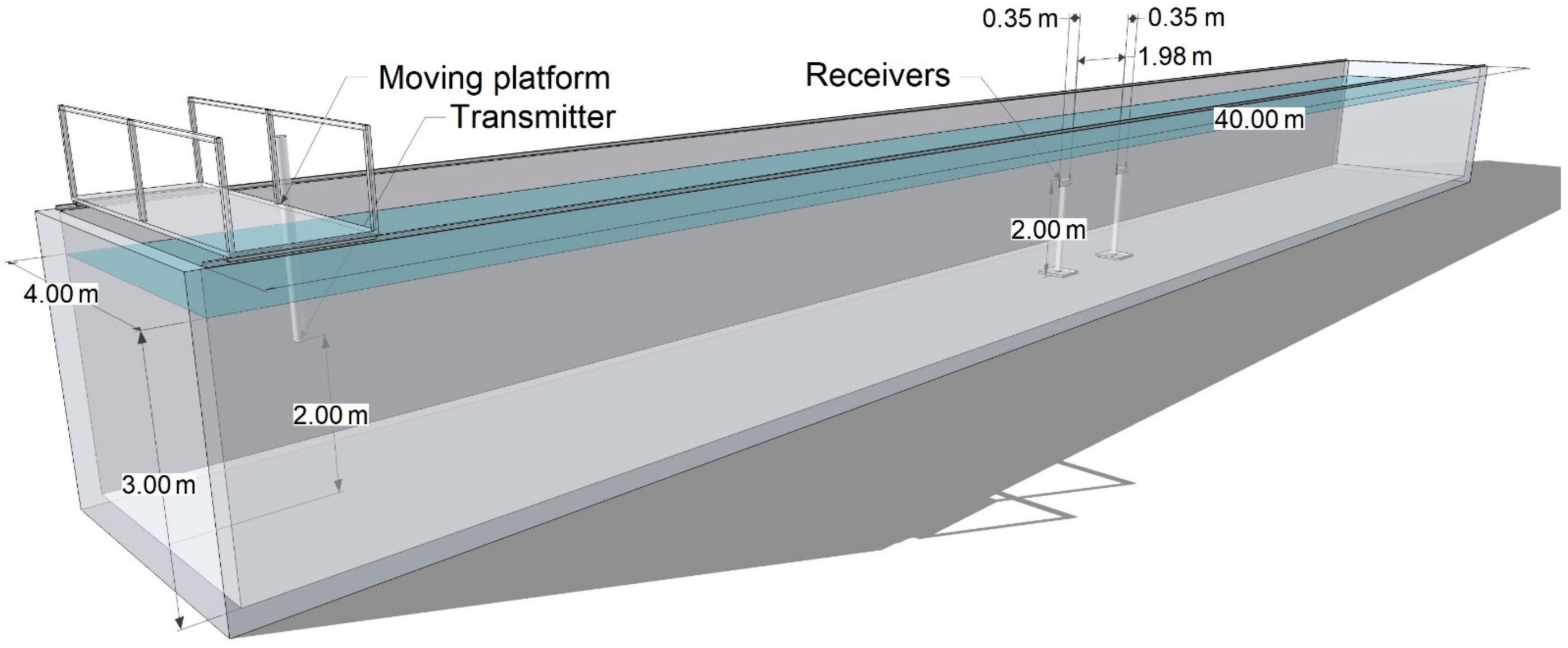
The research was conducted in the towing tank of the Faculty of Mechanical Engineering and Ship Technology of the Gdańsk University of Technology, presented in Figure 1. The height of the water column was 3 m, the width of the towing tank was 4 m, and its length was 40 m. In the central part of the towing tank, in the line of the transmitter’s movement, four hydrophones were placed 1.5 m from the right wall (looking in the direction of the movement), at a depth of 1 m, in pairs, at a distance of 0.35 m between each other and 1.98 m between the pairs. The transmitting hydrophone was attached to the moving platform and immersed 1 m deep at a distance of 1.60 m from the right wall. The prepared structure allowed the transmitter to move at a speed of 1.5 m/s, with an accuracy of 0.01 m/s.

In the transmitting part of the measurement stand, the signal was digitally formed in a Matlab environment and sent via an NI USB-6366 DAC to an ETEC PA1001 amplifier and further to a Reson TC4013 hydrophone. The receiving part consisted of four independent lines with a Reson TC4013 hydrophones-1 piece, a Reson TC4034-1 piece, and Reson TC4014-2 pieces. The lines with the Reson TC4013 and Reson TC4034 hydrophones were additionally equipped with a Reson VP1000 amplifier. The NI USB-6366 card connected to the computer on which the signals were recorded was used as an analog-to-digital converter.

For the purposes of analyzing the recorded signals, the speed of the sound propagation in the water was measured using an STD/CTD SAIV AS SD204 probe. During the measurements, this speed was constant and equal to 1477 m/s.

In the hydroacoustic channel, the transmitted signal propagates along $L$ deterministic paths. The impulse response, $h_{}\left(\tau \right)$, characterizes the multipath propagation, which means that it describes the $l$-th path into which the generated signal splits in response to random inhomogeneities of the medium, i.e., the presence of obstacles. Every replica, because of the specific distance from the transmitter to the receiver, will cause a delay of the signal in the reception point by time ${\tau }_l$. Additionally, during the relative movement of the transmitter and receiver, we have to take into account the Doppler effect. Let parameter ${\eta }_l$ describe the Doppler shift in the $l$-th path.

The equation describing the channel model can be written as follows [22,23]:

$$y\left(t\right)={{\displaystyle \sum }}_{l=1}^{L}x\left({\eta }_{l}t-{\tau }_l\right)h\left({\tau }_l\right)+n\left(t\right),$$

(1)

where $x\left(t\right)$ is the transmitted signal, $y\left(t\right)$ is the received signal, and $n\left(t\right)$ is the additive noise.

The Doppler scattering of the signal is accounted for in (1) by summing the terms with various values of the Doppler parameter, ${\eta }_l$. Parameters ${\tau }_l$ and ${\eta }_l$ and the impulse $h_{}\left(\tau \right)$ vary within a measurement session. In ideal stationary conditions, this parameter should not change in time. In static real conditions, they are assumed to be fixed within the time interval $T_s$, corresponding to the processing of each separate signal.

In our experiments, we used logarithmic chirp signals, where the frequency of the signal varies exponentially as a function of time [24]:

$$f_i\left(t\right)=f_0{k}^t,$$

(2)

where

$$k={\left(\frac{f_1}{f_0}\right)}^{\frac{1}{T}},$$

(3)

where $f_0$ is the starting frequency, $f_1$ is the ending frequency, and $T$ is the sweep time.

It must be noted that $\left|f_0-f_1\right|=B$ is a band occupied by the chirp, and $f_C=f_0+\frac{f_1-f_0}{2}$ is the central frequency of the chirp.

The corresponding time-domain function for the phase of a logarithmic chirp is the integral of the frequency, so we can finally write:

$$\varphi \left(t\right)={\varphi }_0+2\pi f_0\left(\frac{k^t-1}{\ln \left(k\right)}\right),$$

(4)

where ${\varphi }_0$ is the initial phase (at $t=0$).

The corresponding time-domain function for a logarithmic chirp is the sign of the phase:

$$x\left(t\right)=\sin \left(\varphi \left(t\right)\right),$$

(5)

We assume that if $f_0<f_1$, i.e., the frequencies will change from low to high, we will talk about a chirp-up; otherwise, if $f_0>f_1$, i.e., the frequencies will change from high to low, we will talk about a chirp-down.

To estimate the impulse response of a UWA channel, we can use a matched filter. A matched filter is obtained by correlating a known delayed transmitted signal (template) with a received signal. This is equivalent to convolving the received signal with a conjugated time-reversed version of the template $x^{\ast }\left(-t\right)$. It allows us to detect the presence of the template in the received signal. According to the above estimate of an impulse response of a UWA channel, $h\left(\tau \right)$ can be expressed as follows [25]:

$$h\left(\tau \right)={{\displaystyle \int }}_{-\infty }^{+\infty }{x}^{\ast }\left(-t+\tau \right)y\left(t\right)dt,$$

(6)

The matched filter is a linear filter that maximizes the output signal-to-noise ratio.

3. Evaluation of the Stationarity of the UWA Channel

Logarithmic chirp signals, which were emitted at the same time and on the same central frequency, were used to assess the stationarity of the channel. The measure of stationarity is the value of the cross-correlation of the impulse response determined for the chirp-up and chirp-down signals normalized to the root of the product of the maximum auto-correlation values of the impulse responses obtained from the chirps up and down. This coefficient can be described by the equation:

$${\widehat{R}}_{UD,coeff}=\frac{\max \left({\widehat{R}}_{UD}\left(m\right)\right)}{\sqrt{{\widehat{R}}_{UU}\left(0\right) {\widehat{R}}_{DD}\left(0\right)}},$$

(7)

where $R_{UU}\left(0\right)$ is the maximum of the autocorrelation for the estimation of the impulse response determined by a chirp-up; $R_{DD}\left(0\right)$ is the maximum of the autocorrelation for the estimation of the impulse response determined by a chirp-down; $R_{UD}\left(m\right)$ is the cross-correlation for the estimation of the impulse response determined by a chirp-up and a chirp-down.

A channel is considered stationary when the similarity coefficient, ${\widehat{R}}_{UD,coeff}$, is greater than $0.5$.

3.1. Simulation Research

The validation of the proposed solution of evaluating the stationarity of the hydroacoustic channel was carried out with the use of a UWA channel available in the Matlab computing environment library. The documentation of the UWA channel simulator shows that for the duration of the transmitted signal, the channel is a stationary one, i.e., the parameters determined for the individual paths do not change over time. Using this model, we can confirm that the proposed method allows for the determination of stationarity. The simulations were performed for the case of the transmitter moving in relation to the receiver. The simulation main parameters were as follows:

• The distance between the receiver and transmitter was 900 m;
• The channel depth was 6 m;
• The underwater sound propagation speed was 1470 m/s;
• The receiver immersion depth was 1 m;
• The transmitter immersion depth was 2 m;
• The source velocity was 15 m/s.

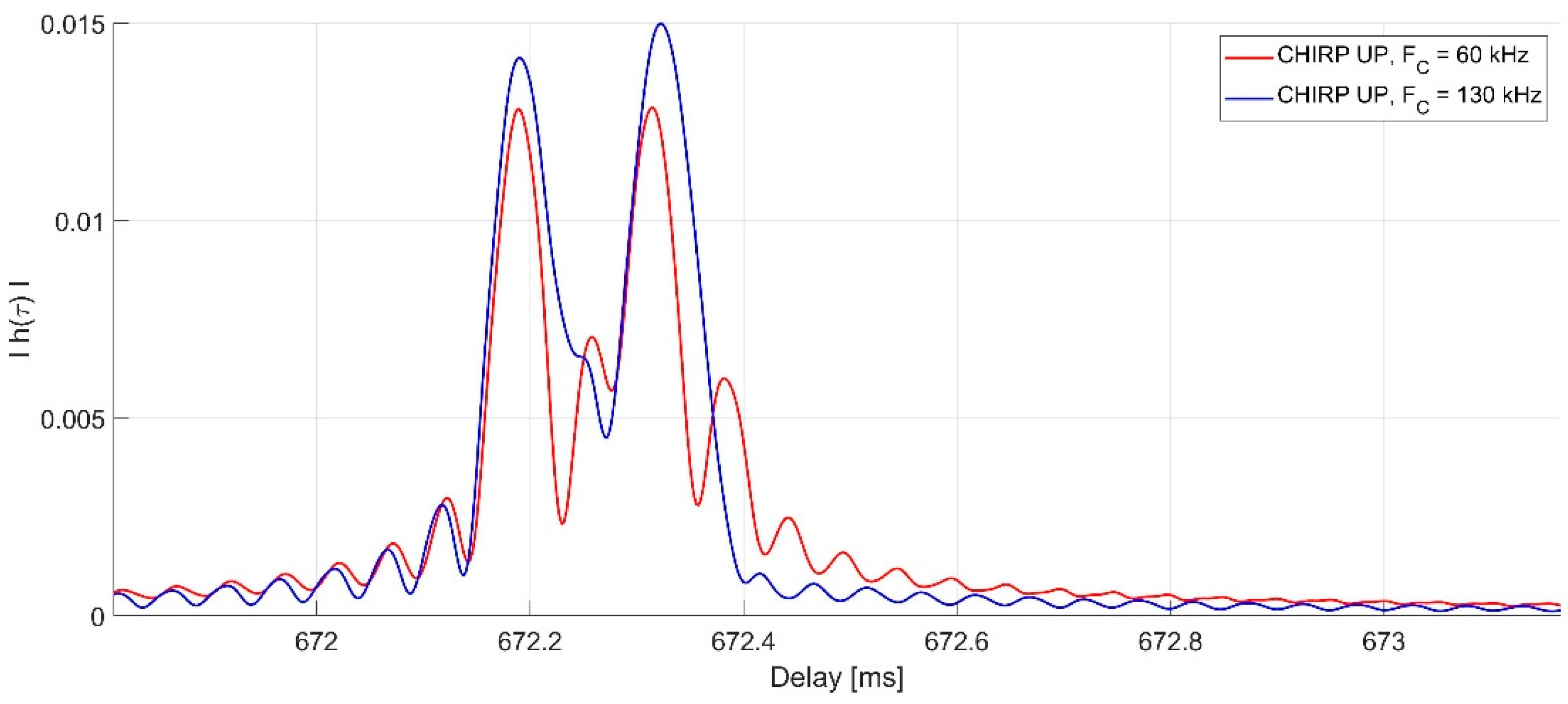
The estimates of the impulse responses obtained with the utilization of the chirp-up signal with different carrier frequencies tend to be radically different, as can be clearly seen in Figure 2.

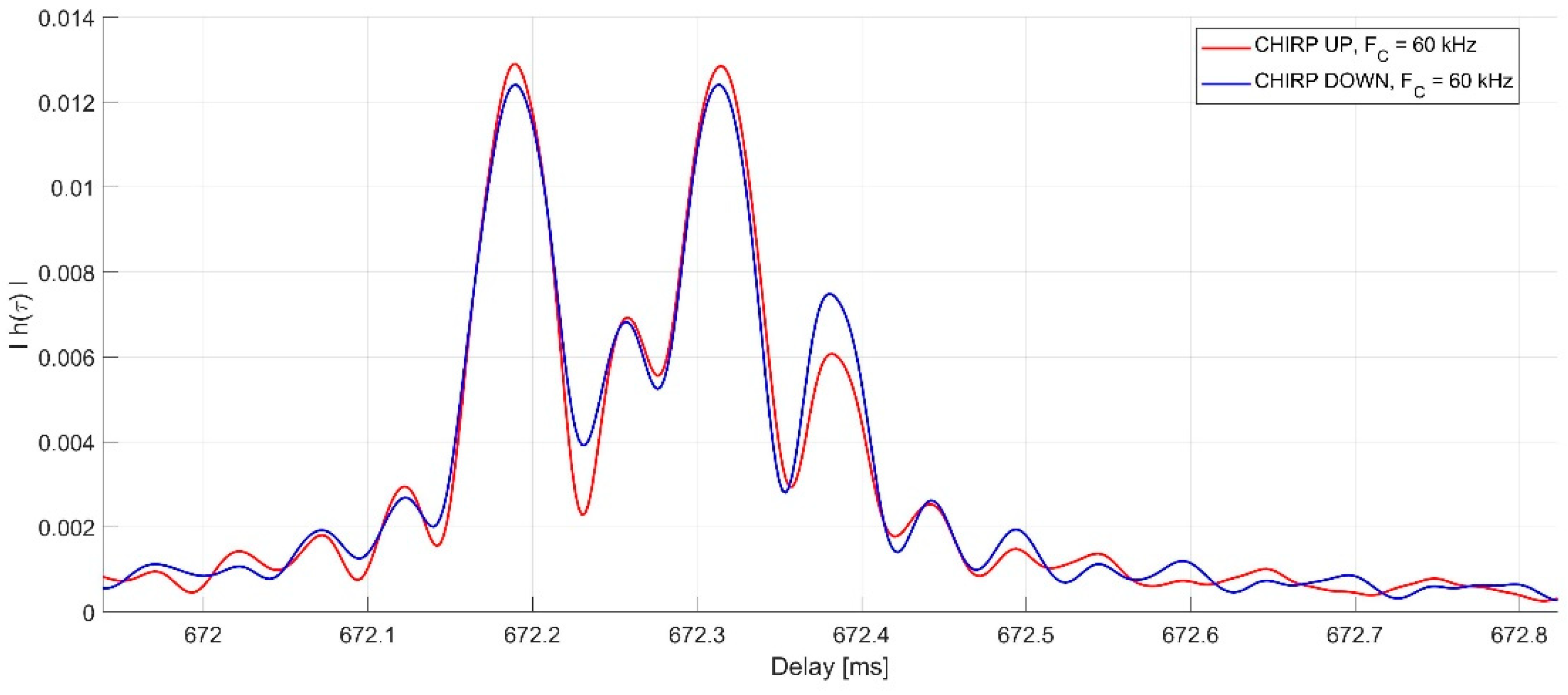
In this case (shown in Figure 2), the determined value of the similarity coefficient is 0.952. Under the same conditions, chirp-up and chirp-down signals were sent at the same time on the same center frequency (see Figure 3). In this case, the similarity coefficient is 0.993.

It should be noted that although the channel did not change, a lower similarity coefficient was obtained in the case where two different center frequencies were used. On this basis, it was assumed that, in further research, we will use chirp-up and -down signals transmitted at the same time and on the same central frequency.

3.2. Evaluation of the Stationarity of the Measurement Channel

The stationarity of the measurement channel was evaluated in motion for the following transmitter speeds: 0.25 m/s, 0.5 m/s, 1 m/s, and 1.5 m/s. The measurement signal was generated at three different center frequencies: the $F_C$ i.e., 50 kHz, 95 kHz and 140 kHz in band $B$ equals 2 kHz, 10 kHz, 20 kHz, and 40 kHz, and the duration time, $T$, equals 30 ms or 60 ms.

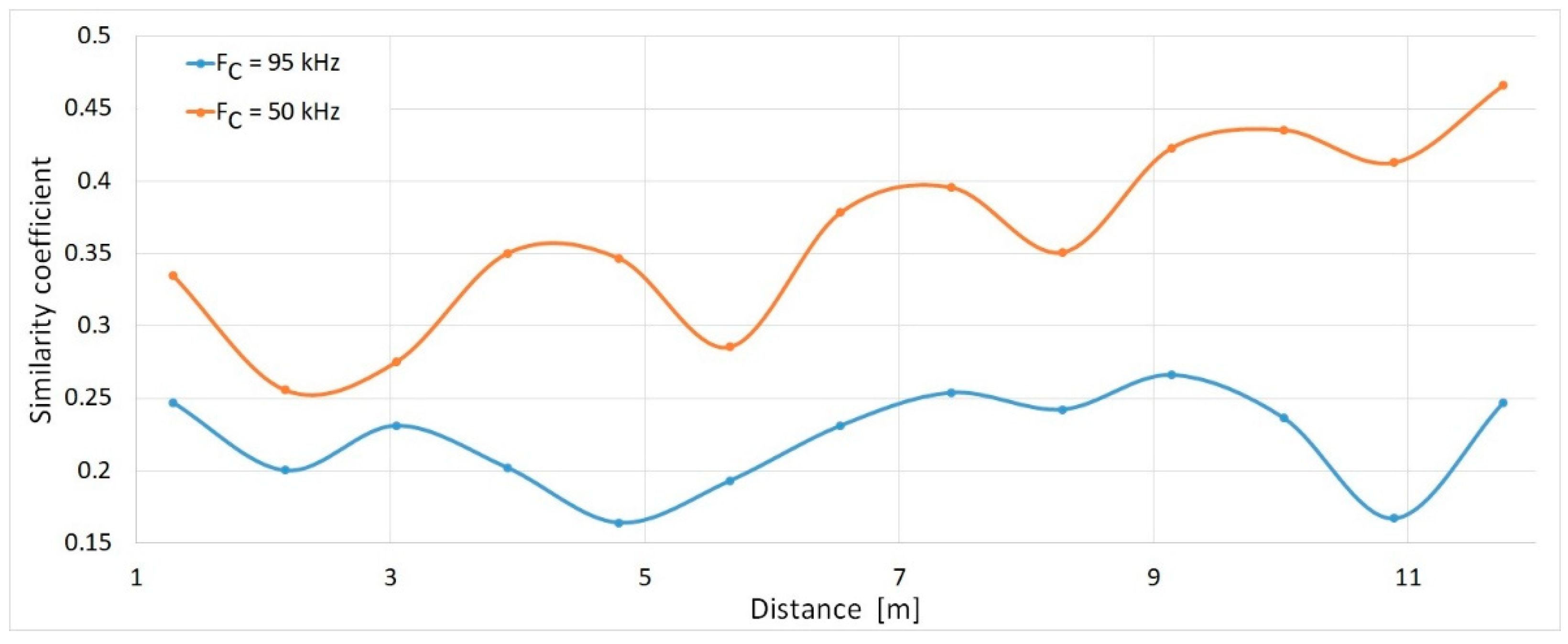
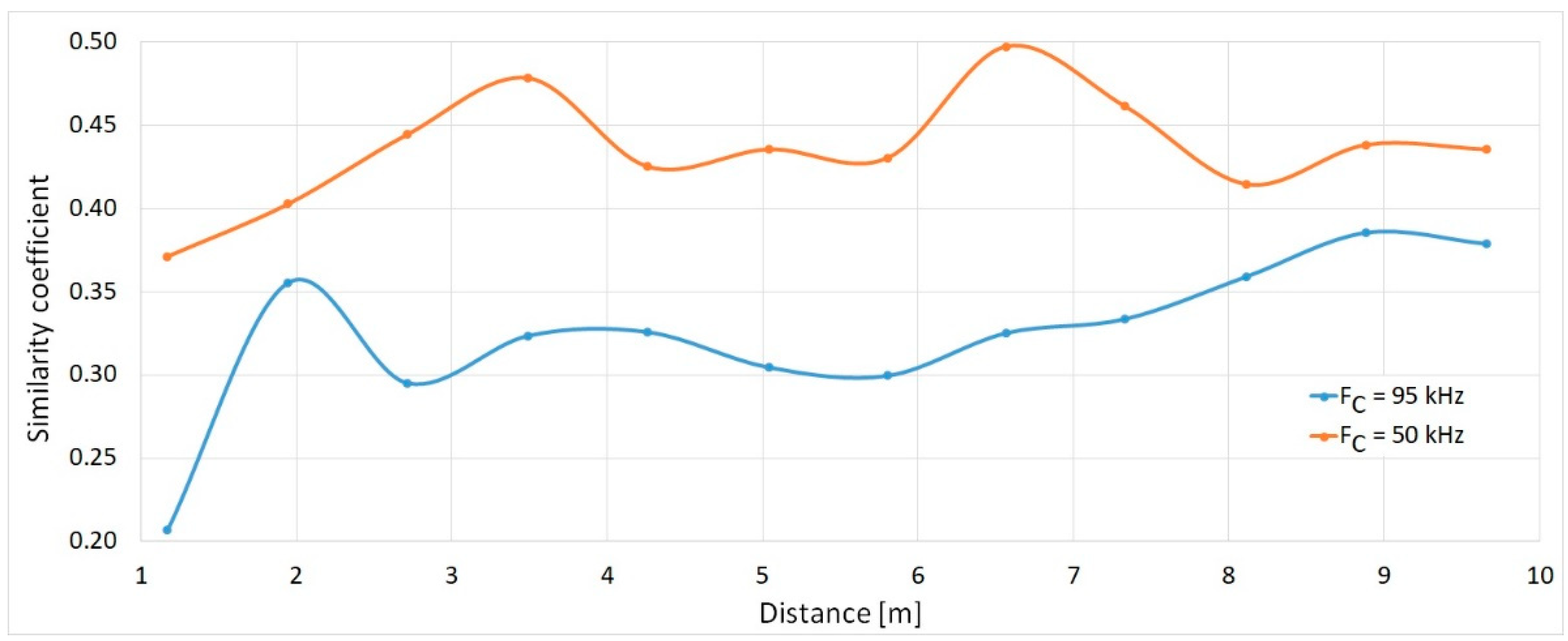
Figure 4 shows the average (from four receivers) values of the measured similarity coefficients as a function of the distance from the receiver for the transmitter speed of $V=1 \mathrm{m}/\mathrm{s}$ and band $B=20 \mathrm{kHz}$ and the duration of the measurement signal $T=60 \mathrm{ms}$.

The obtained results indicate that at the velocity $V=1 \mathrm{m}/\mathrm{s}$ for the chirp band $B=20 \mathrm{kHz}$ and the duration $T=60 \mathrm{ms}$ at a distance from $1 \mathrm{m}$ to $12 \mathrm{m}$ from the receiver, the channel was non-stationary, both for the center frequency $F_C=50 \mathrm{kHz}$ and $F_C=95 \mathrm{kHz}$.

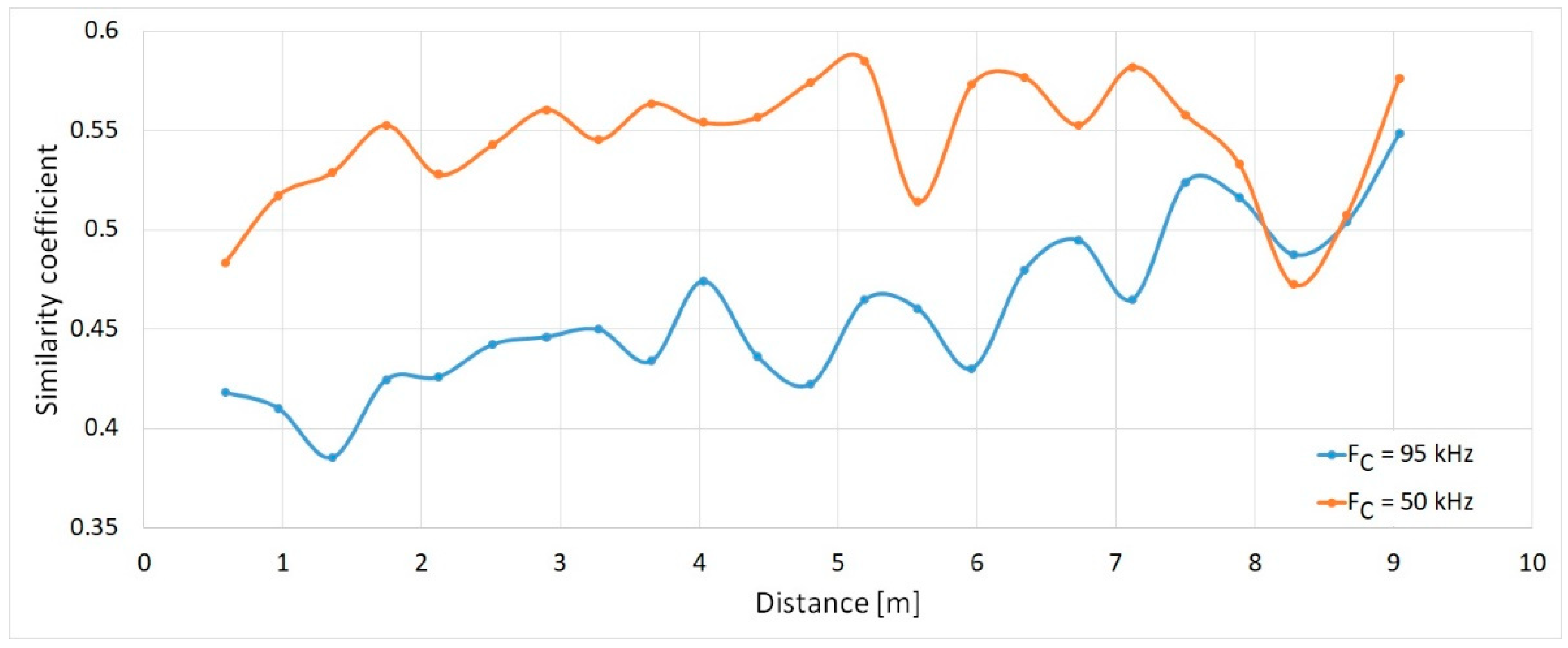
Figure 5 shows the average, from the four receivers, values of the measured similarity coefficients as a function of the distance from the receiver for the transmitter speed as before, i.e., $V=1 \mathrm{m}/\mathrm{s}$, but the band was smaller and equals $B=10 \mathrm{kHz}$, and the duration of the chirp signal, $T$, was $30 \mathrm{ms}$.

The measurement results presented in Figure 5 show that despite the narrower band $B=10 \mathrm{kHz}$ and a shorter chirp duration for two times, the channel was also non-stationary; however, the achieved similarity coefficients in Figure 5 are greater compared to those in Figure 4.

Figure 6 shows the average (from four receivers) values of the measured similarity coefficients as a function of the distance from the receiver for the transmitter velocity of $V=0.5 \mathrm{m}/\mathrm{s}$ in the band of $B=20 \mathrm{kHz}$ and the duration of the chirp of $T=30 \mathrm{ms}$.

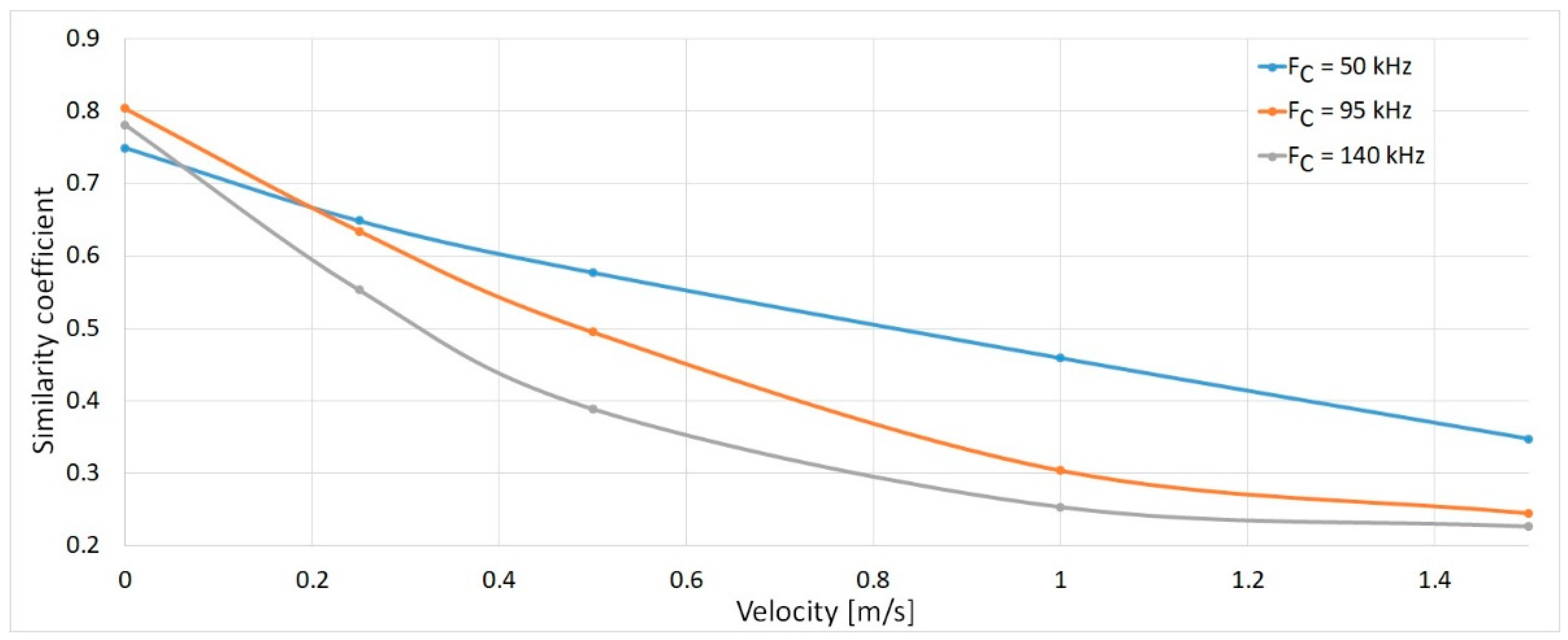
From the obtained results, it can be concluded that by reducing the velocity of a moving transmitter, the values of the similarity coefficient are greater than those measured at higher velocities. From the above, it should be considered that the stationarity of the channel cannot be unambiguously associated with the distance between the transmitter and the receiver. Therefore, for each velocity, the similarity coefficients from all distances from the transmitter were averaged (Figure 7).

When comparing the values of the similarity coefficient for different velocities of the transmitter, it can be seen that for $B=20 \mathrm{kHz}$, only at the speed of $V=0.25 \mathrm{m}/\mathrm{s}$ and in static conditions (the transmitter did not move) for all of the analyzed center frequencies, the stationarity of the UWA channel was found.

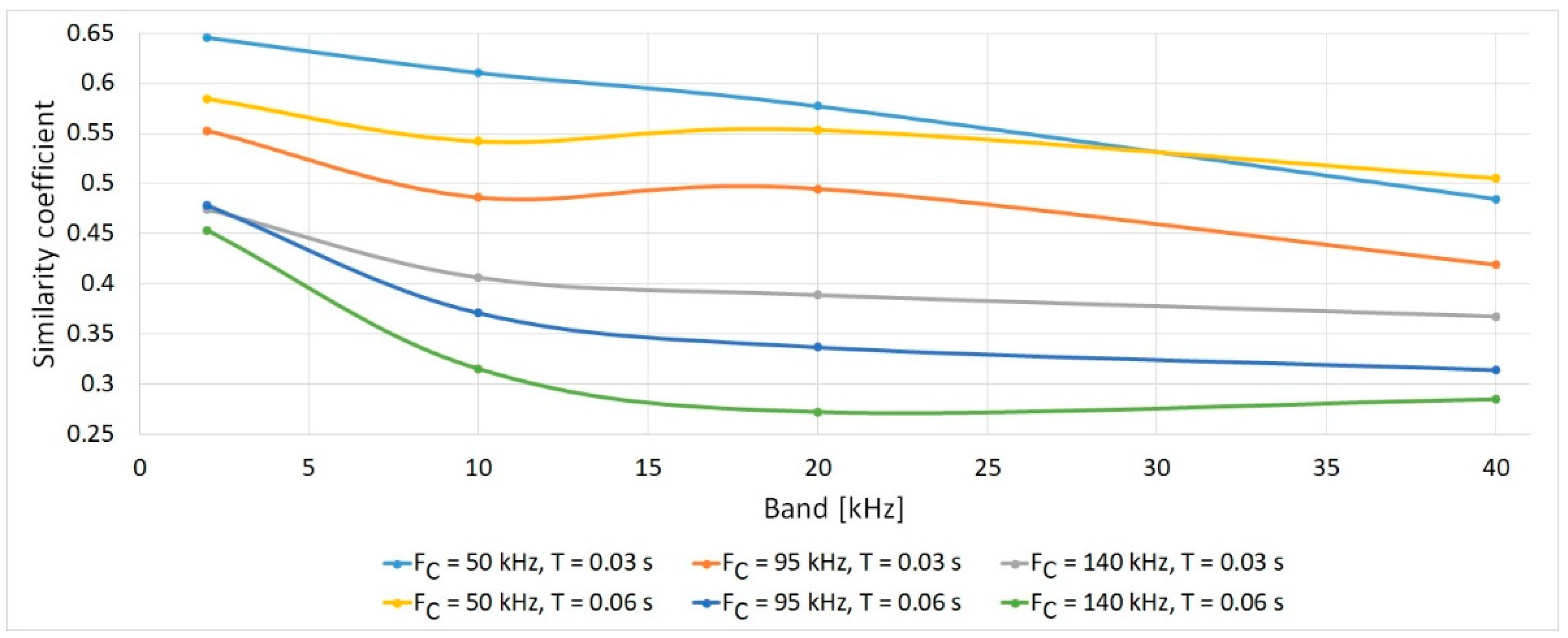
Figure 8 shows the assessment of the influence of the measurement signal bandwidth on the value of the similarity coefficient.

Based on the research results presented in Figure 8, it can be seen that the narrower the bandwidth occupied by the signal and the shorter its duration, the easier it is to ensure channel stationarity. Also, as the center frequency of the signal increases, the channel becomes non-stationary.

The analysis of the results presented in Figure 4, Figure 5, Figure 6, Figure 7 and Figure 8 shows, as should be expected, that the higher the speed of the transmitter’s movement in relation to the receiver, the longer the signal duration, and the greater the bandwidth, the more difficult it is to ensure the channel stationarity.

4. Research Results

The analysis of the impulse response parameters measured in motion was performed using the measurement stand and under the conditions described in Section 2. Single logarithmic chirp signals were transmitted to obtain complex impulse responses. It should be noted that two signals were not sent simultaneously, i.e., up and down, at the same time and at the same center frequency, as it was conducted in the evaluation of the stationarity of the UWA channel (Section 3). Thus, the impulse response was not overloaded. That is, on a given center frequency, the sequence of up/down/up-chirps were successively transmitted with an interval of $100 \mathrm{ms}$ between them. Then, such a set of measuring signals was repeated with a time interval of $500 \mathrm{ms}$. 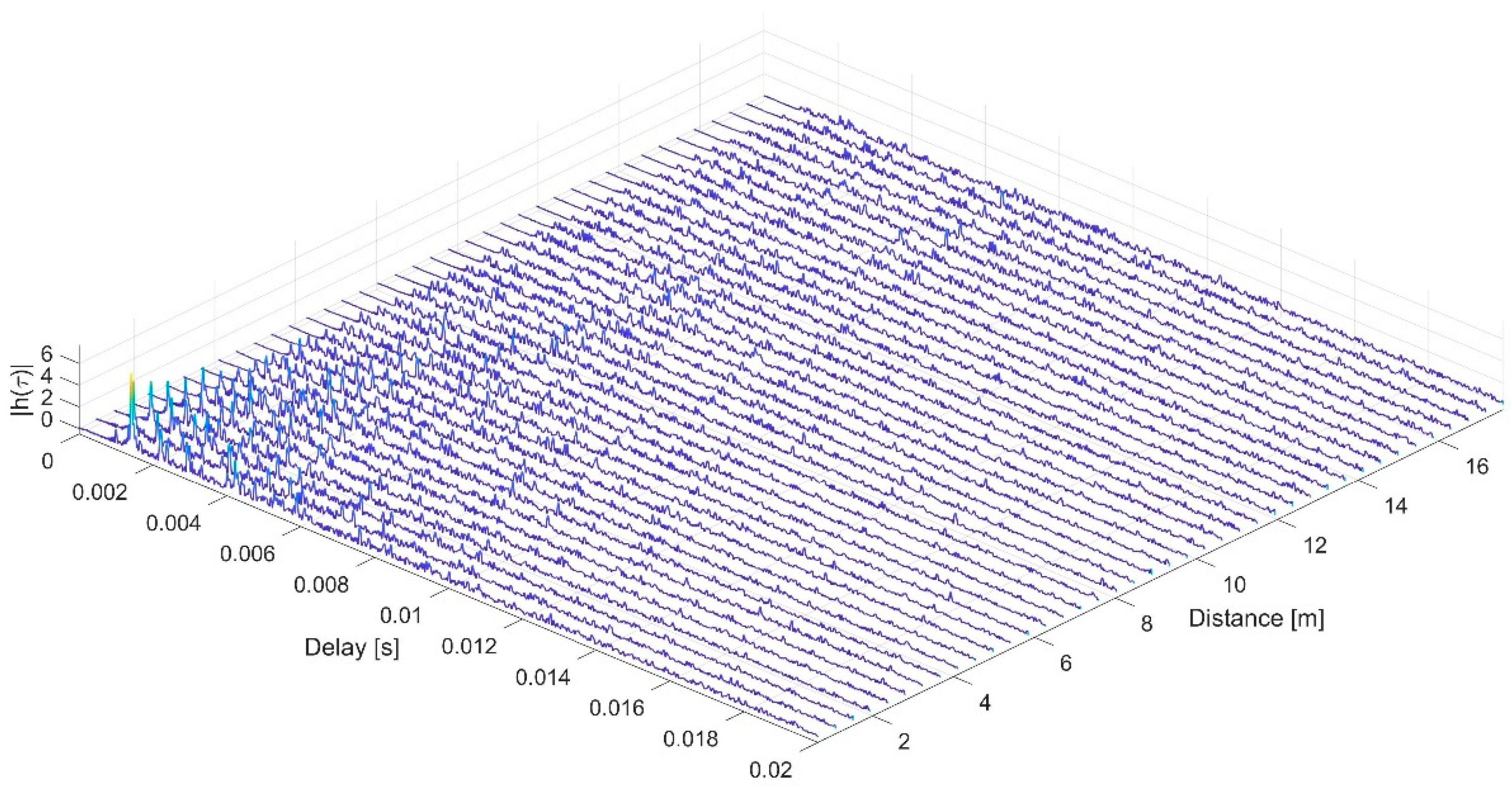Figure 9 shows an example of the registered impulse responses in the first measurement channel during the transmitter’s approach to the receiver.

The obtained result clearly shows that as the transmitter gets closer to the receiver, the strength of the received signal increases, and the delay between the signal arriving directly from the direct route and the replicas increases. This is because the direct path of signal propagation from the transmitter to the receiver is shortened, e.g., when the transmitter passes the receiving hydrophone, then, in the adopted measurement configuration, the first replica, reflected from the water surface, must cover a distance of 2 m.

By analyzing the impulse responses measured in motion, the mean square delay spread, ${\tau }_{rms}$, and the number of replicas were determined.

The root mean square delay spread, ${\tau }_{rms}$, was determined according to the equation [26]:

$${\tau }_{rms}=\sqrt{\frac{{{\displaystyle \sum }}_{i=1}^N{\tau }_i^{2}p\left({\tau }_i\right)}{P_m}-{\overline{\tau }}^2},$$

(8)

where $p\left({\tau }_i\right)$ is the power of the $i$-th replica, $N$ is the number of replicas, and $\overline{\tau }$ is the average delay of the received replicas, which can be calculated according to the following equation [26]:

$$\overline{\tau }=\frac{{{\displaystyle \sum }}_{i=1}^N{\tau }_{i}p\left({\tau }_i\right)}{P_m},$$

(9)

where $P_m$ is the total power of all signal replicas in a single impulse response, described by equation [26]:

$$P_m={{\displaystyle \sum }}_{i=1}^{N}p\left({\tau }_i\right).$$

(10)

Only those replicas whose level was not lower than −15 dB in relation to the signal with the highest power for the impulse response were taken for analysis, which is in line with the recommendation of ITU-R P.1407-7 [26]. All recorded signals were subjected to resampling before determining the impulse response. The resampling was performed on the basis of the measured speed of the sound in the water and the current speed of the transmitter. The aim of this procedure was to minimize the influence of the Doppler effect on the form of the final impulse response estimates.

4.1. Analisis of Number of Replicas

The assessment of the number of replicas meeting the conditions in accordance with Recommendation ITU-R P.1407-7 was carried out as a function of the transmitter velocity, $V$, the bandwidth occupied by the chirp signal, $B$, the center frequency, $F_C$, the chirp duration, $T$, and the distance between the transmitter and receiver.

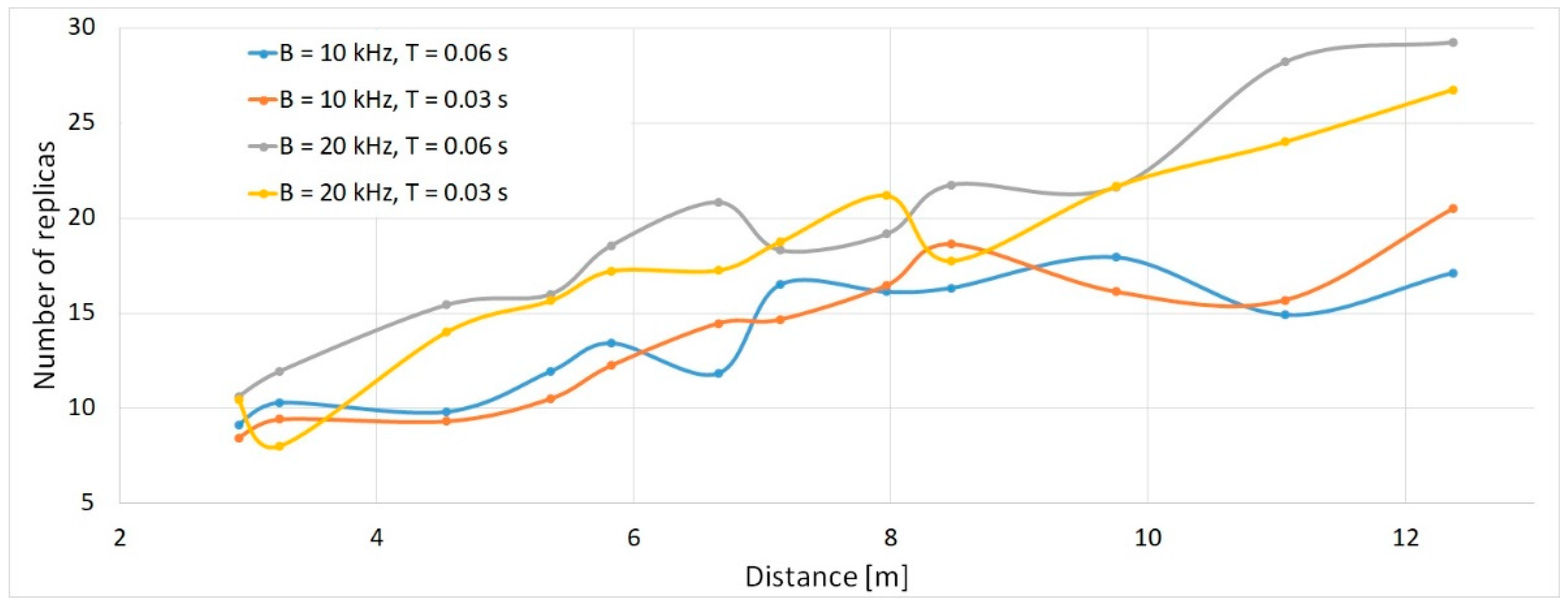
Figure 10 shows the relation between the number of replicas and the distance for different bandwidths, $B$, and the duration of the chirp, $T$, at the transmitter’s speed of $V=1.5 \mathrm{m}/\mathrm{s}$.

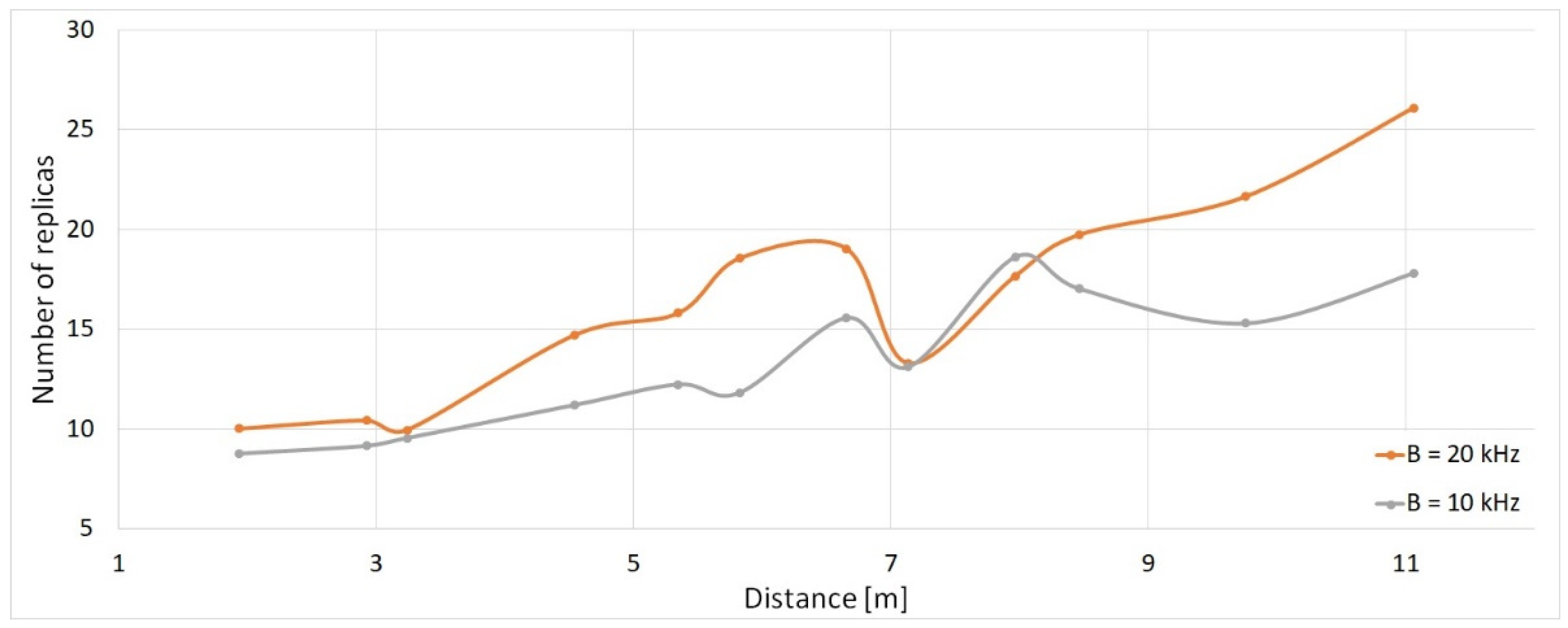
The obtained result shows that the number of replicas does not depend on the chirp duration but depends on the bandwidth of the measurement signal. This relationship results from the fact that the wider the bandwidth, $B$, the greater the resolution of the obtained impulse response estimate, and as a result, the greater the number of distinguished replicas. Therefore, the results for different chirp durations can be averaged. Another example of this relationship, this time for a speed of $V=1 \mathrm{m}/\mathrm{s}$, is shown in Figure 11.

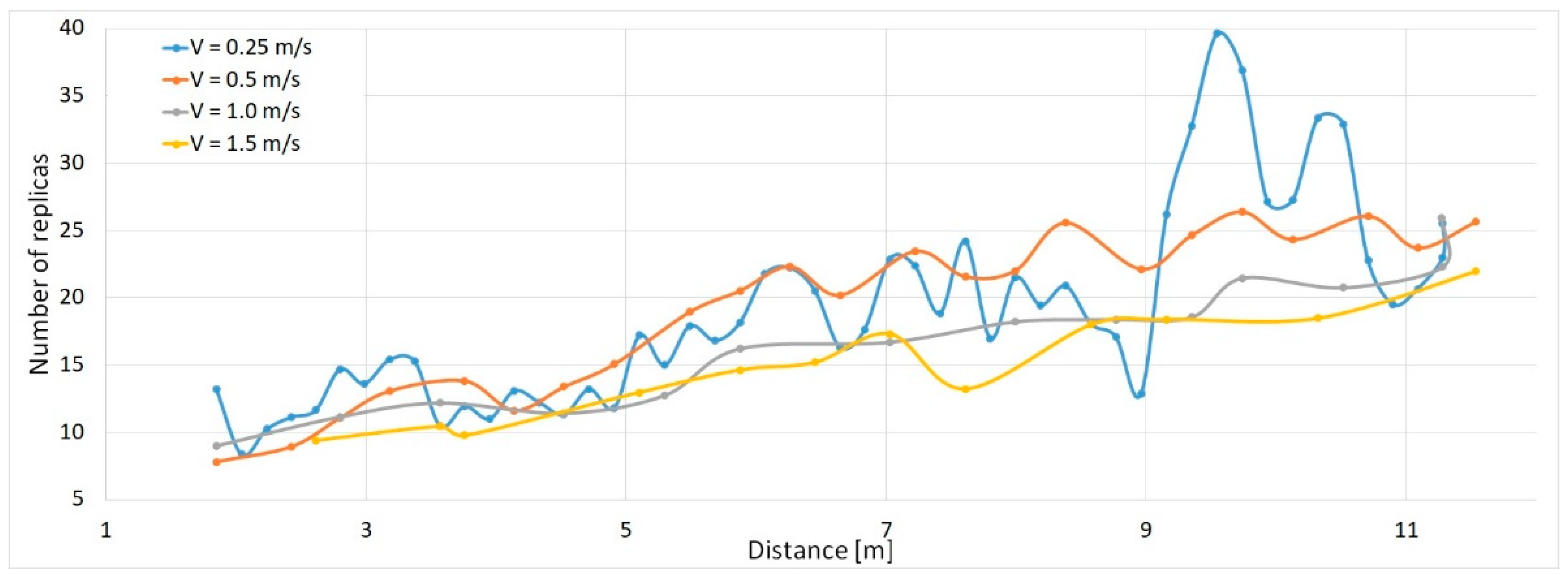
An analysis of the influence of the movement speed of the transmitter relative to the receiver on the number of replicas was also carried out. The result is shown in Figure 12.

The obtained result shows that, in practice, the number of essential replicas in the channel does not depend on the speed.

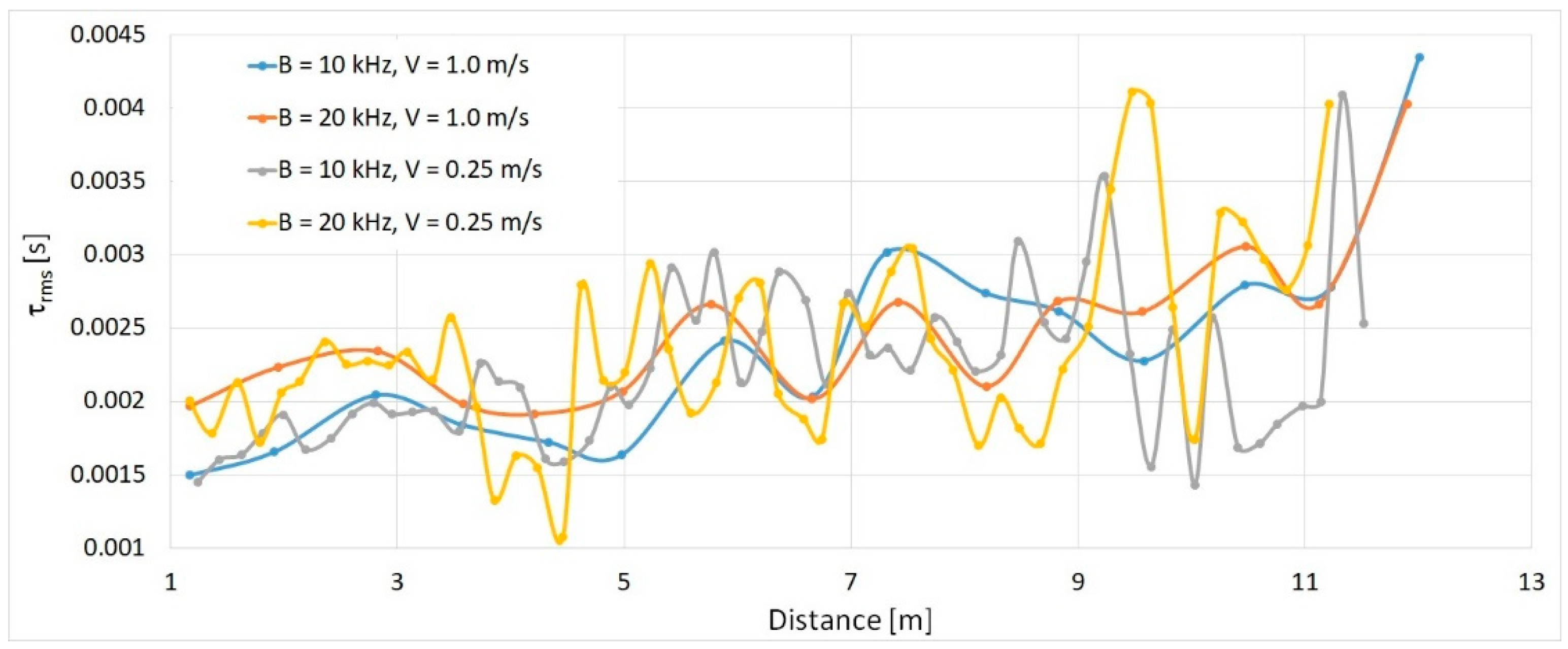
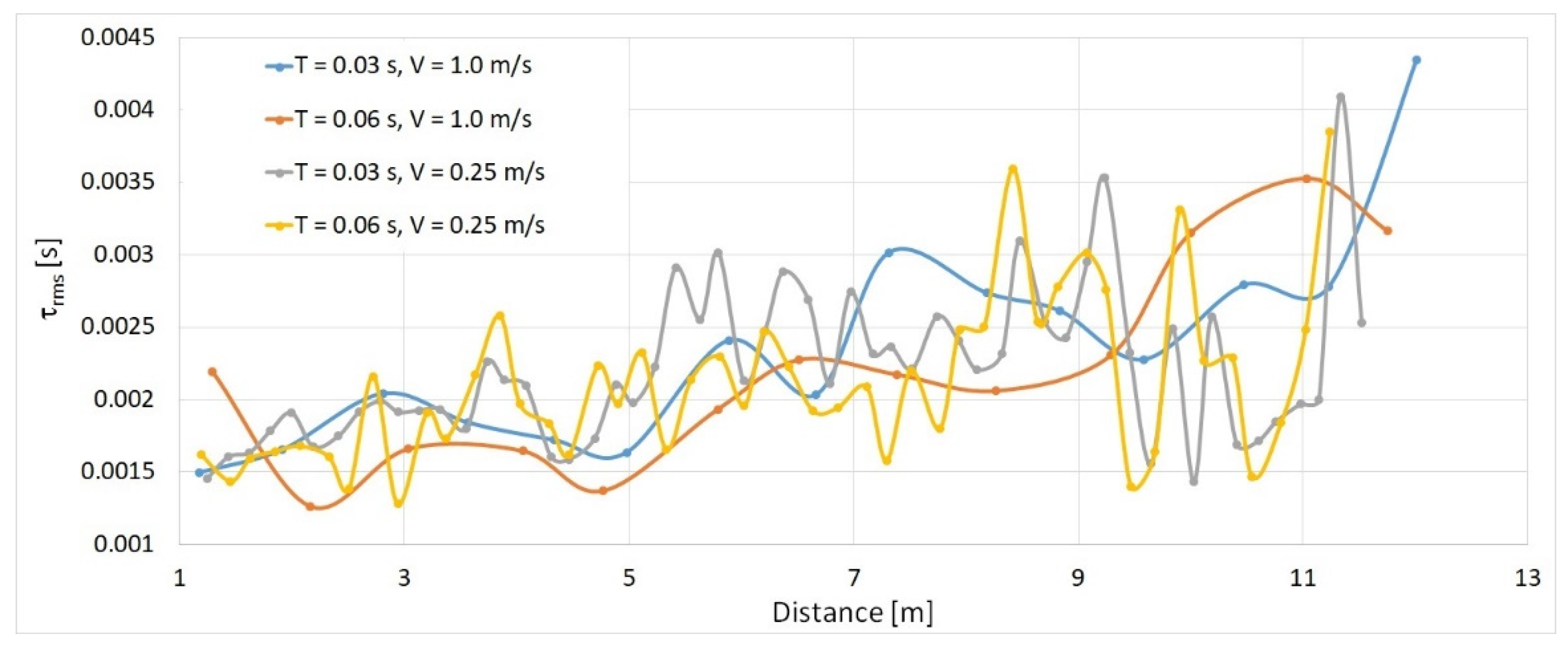
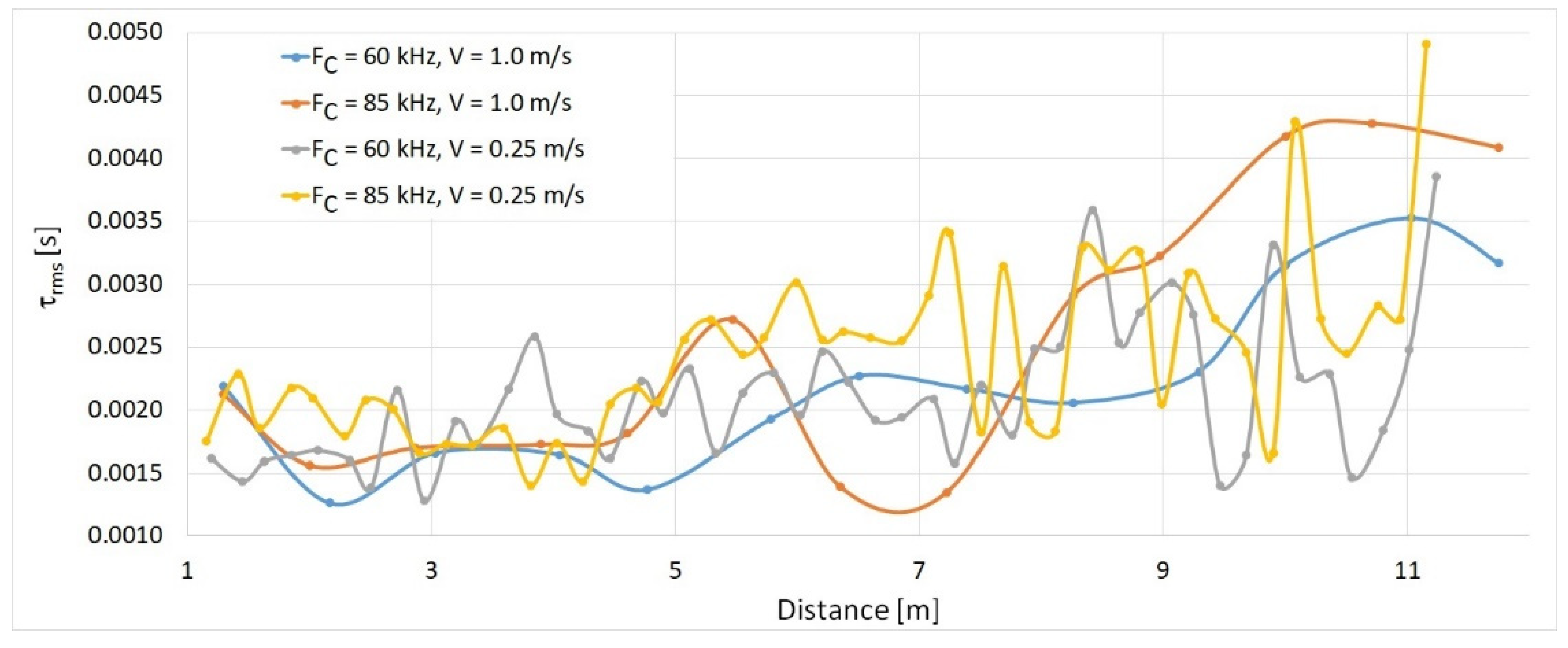
4.2. Analisis of Root Mean Square Delay Spread

In the next stage of the analysis, the values of the root mean square delay spread, ${\tau }_{rms}$, were compared for different transmission speeds of the transmitter and different bandwidths of the measurement signal, center frequency, and duration of the measurement signal as a function of the distance between the transmitter and the receiver. The results are shown in Figure 13, Figure 14 and Figure 15.

The results shown in Figure 13 show that despite the increase in the number of replicas with the bandwidth, the value of this parameter depends only on the distance.

The presented results show that, regardless of the movement speed of the transmitter relative to the receiver, the delay spread, ${\tau }_{rms}$, does not depend on the bandwidth of the measurement signal, $B$, the center frequency, $F_C$, and the duration of the measurement signal, $T$. It should also be noted that the delay spread, ${\tau }_{rms}$, depends only on the distance between the transmitter and the receiver.

5. Conclusions

The knowledge of the impulse response of the UWA channel is important due to the influence of propagation phenomena on the form of the received signal. With this information, simulation tests can be carried out. This will allow for, among other things, quick and low-cost validation of the operation of underwater systems, which utilize elastic wave propagation. Most of the simulators of acoustic wave propagation in water available today provide data for static scenarios. In the opinion of the authors, this does not correspond to scenarios in motion. Therefore, one of the objectives of the research was to find out about the propagation conditions when the transmitter is moved relative to the receiver. For the authors, this research is an introduction to work on wireless underwater communication systems operating in difficult propagation conditions, e.g., in wrecks or between moving objects.

The aim of the presented research was to determine and analyze the estimates of impulse responses in a towing tank characterized by a strong multipath. In addition, the authors had the possibility to carry out measurements between objects during the movement of the transmitter with a precisely set velocity. As a result of the mutual movement of the receiver and the transmitter, the impulse response changed with the distance between the devices. As a result, a non-stationary channel was obtained, which was confirmed by the proposed method of channel stationarity evaluation. The measurements were conducted for selected speeds of the transmitter {0.0, 0.25, 0.5, 1.0, and 1.5} [m/s], selected central frequencies {50, 60, 85, 90, and 140} [kHz], selected bandwidths {2, 10, 20, 40} [kHz], and chirp duration times {0.03 and 0.06} [s].

Based on the tests carried out in the towing tank, it was found that, despite the fact that they were carried out in a non-stationary channel, one of the most important parameters describing the channel was that the root mean square delay spread did not change as a function of the transmitter movement velocity and the parameters of the generated chirp signal, but only depended on the distance between the transmitter and the receiver.

The complex estimates of the impulse responses obtained as a result of the measurements have been made available as Supplementary Materials to this article.