Augmented Lagrangian-Based Reinforcement Learning for Network Slicing in IIoT

Abstract

Network slicing enables the multiplexing of independent logical networks on the same physical network infrastructure to provide different network services for different applications. The resource allocation problem involved in network slicing is typically a decision-making problem, falling within the scope of reinforcement learning. The advantage of adapting to dynamic wireless environments makes reinforcement learning a good candidate for problem solving. In this paper, to tackle the constrained mixed integer nonlinear programming problem in network slicing, we propose an augmented Lagrangian-based soft actor–critic (AL-SAC) algorithm. In this algorithm, a hierarchical action selection network is designed to handle the hybrid action space. More importantly, inspired by the augmented Lagrangian method, both neural networks for Lagrange multipliers and a penalty item are introduced to deal with the constraints. Experiment results show that the proposed AL-SAC algorithm can strictly satisfy the constraints, and achieve better performance than other benchmark algorithms.

1. Introduction

With the rapid development of industrial internet of things (IIoT), more and more devices are connected and controlled via wireless networks. Providing precise services for these devices to fulfill their diverse requirements becomes a fundamental issue in IIoT. Facing this challenge, three application scenarios are defined by International Telecommunication Union (ITU) and Fifth Generation Public Private Partnership (5G-PPP) [1,2], that is, enhanced mobile broadband (eMBB), ultra-reliable low latency communications (URLLC), and massive machine type communication (mMTC). In more detail, the eMBB scenario provides devices with requirements on high transmission rate, such as high-definition surveillance video in factories, whose peak rate for each camera can be greater than 10 Gbps [3]. mMTC refers to the scenarios, where a large number of devices connect simultaneously while the requirements on the transmission rate and delay are not critical [4]. In contrast, URLLC serves applications with a strict transmission on reliability, and latency, such as automatic operators and controllers [5].

To satisfy these disparate scenarios within one network infrastructure, a network slicing technique was proposed. It divides a physical network into multiple independent logical networks [6,7], where each network slice is isolated from others and provides one kind of network service via dedicated resource allocation. To efficiently allocate resources and meet the dynamic of wireless networks, many intelligent algorithms have been proposed. For instance, in [8], the genetic algorithm, ant colony optimization with a genetic algorithm, and quantum genetic algorithm were used to jointly allocate radio and cloud resources to minimize the end-to-end response latency experienced by each user. In [9], two deep learning technologies, supervised and unsupervised learning, were introduced to jointly optimize user association and power allocation problems, combining the data-driven and model-driven learning. The study in [10] exploited a learning-assisted slicing and concurrent resource allocation process to jointly to improve the users’ service reliability and resource utilization rate.

Following 5G network architecture, edge servers with caching and computing capacities are deployed close to the base stations (BSs). Such kinds of deployment enables the intelligent cooperative among the neighboring BSs, which is suitable for the network slicing for an intelligent factory. Resource allocation is a dynamic programming problem, which can also be solved effectively by reinforcement learning (RL). In [11], RL was utilized to dynamically update the number of radio resource units allocated to each slice, where a utility-based reward function was adopted to achieve efficient resource allocation. Cooperative proximal policy optimization was adopted in RL to maximize resource efficiency by considering different characteristics of the different network slices in [12]. A general framework was proposed in [13] that uses RL to achieve dynamic resource management of dynamic vehicle networks in realistic environments. Moreover considering the high complexity and combinatorial nature of the future heterogeneous networks consisting of multiple radio access technologies and edge devices, a  multi-agent DRL-based method was utilized in [14,15]. Specifically, in [14], deep Q-network (DQN) algorithm was used in each agent to assign radio access technologies, while the multi-agent deep deterministic policy gradient (DDPG) algorithm to allocate power. The authors in [15] investigated a multi-agent cooperative problem in resource allocation aiming at improving the data process ability of wireless sensor networks and eliminating the non-stationary problem for channel allocation.

However, resource allocation problems in a wireless network always involve constraints, e.g., the device’s various requirements on average latency, cumulative throughput, or the average package loss rate, which cannot be solved well by traditional RL. To manage the constraints, constrained Markov decision processes (CMDP) arose, which mainly include four classes: (1) penalty function method: it adds penalty terms into the optimization objective to construct an unconstrained optimization problem. Such as in [16], the logarithmic barrier function is introduced as a penalty. (2) Primal- dual method: it uses the Lagrangian relaxation technique to transform the original problem into a dual problem, for instance [17,18]. (3) Direct policy optimization: it replaces the objective or constraint in the original problem by a more tractable function, such as  [19,20,21]. (4) Safeguard uses an extra step mechanism to guarantee the constraint in each training step [22].

In addition to the constraint problem, the discrete-continuous mixed action space is involved in our work. Inspired by the concepts of the augmented Lagrangian similar to the primal-dual method, we propose an augmented Lagrangian-based soft actor–critic (AL-SAC) algorithm to solve the network slicing problem with constraints and the hybrid action space. The main contributions of this paper are as follows.

• A two-stage action selection is designed by considering a hierarchical policy network to solve the hybrid action space problem in RL, which can significantly reduce the action space;
• A penalty-based piece-wise reward function and a constraint-handling part involving neural networks for Lagrangian multipliers and cost functions are introduced to solve the constraint problem;
• Simulation results show that our proposed algorithm satisfies the constraints, and AL-SAC has a higher reward value than the DDPG algorithm with a penalty item.

2. System Model and Problem Formulation

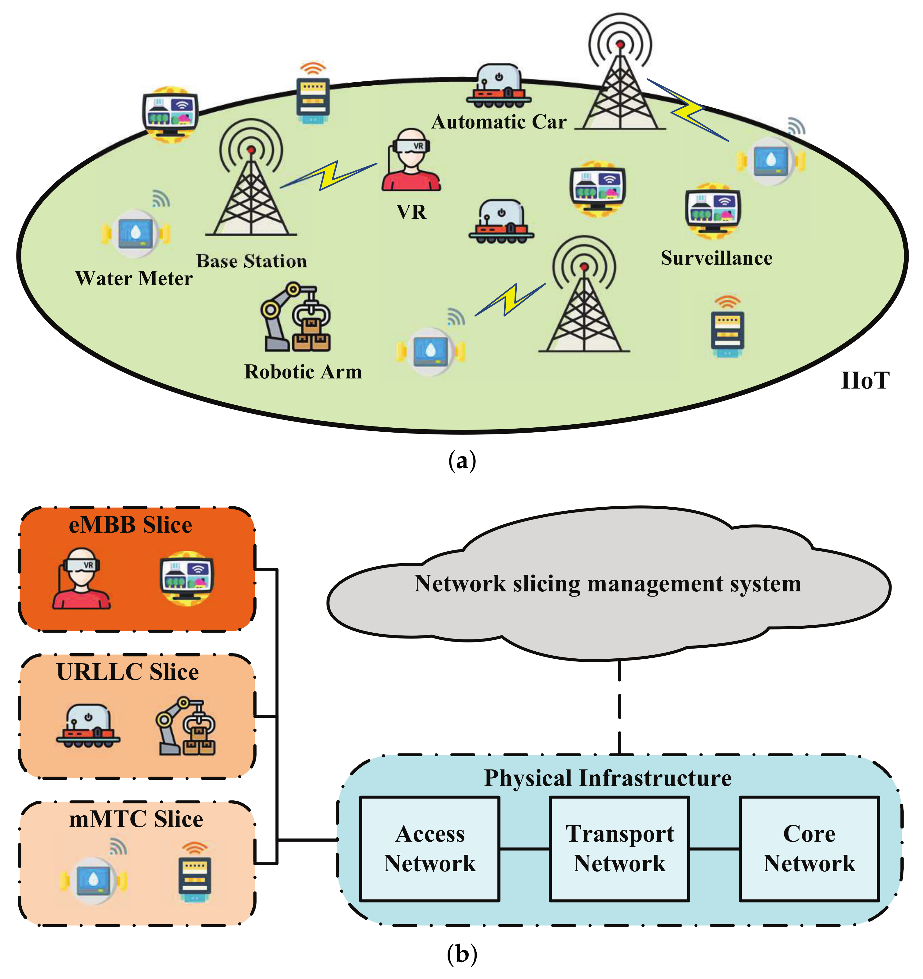
This section firstly presents the network model of network slicing and transmission rate model. Then, considering various requirements of different network slices, the constraints of different types of devices are developed. Finally, a constrained mixed integer nonlinear problem is formulated.

2.1. Network Model

As illustrated in Figure 1, we consider a wireless IIoT with multiple BSs and devices with different network requirements. We denote the set of BSs and devices by $\mathcal{M}=\{1,2,\cdots ,M\}$ and $\mathcal{N}=\{1,2,\cdots ,N\}$. Moreover, the devices are categorized into three typical scenarios, i.e., eMBB, mMTC, and URLLC, which are denoted by ${\mathcal{N}}_{\mathrm{eM}}$, ${\mathcal{N}}_{\mathrm{uR}}$ and ${\mathcal{N}}_{\mathrm{mM}}$, respectively. Hence, ${\mathcal{N}}_{\mathrm{eM}}\cup {\mathcal{N}}_{\mathrm{uR}}\cup {\mathcal{N}}_{\mathrm{mM}}=\mathcal{N}$.

We further denote the bandwidth available in the m-th BS by $B_m$, $m\in \mathcal{M}$, and its transmission power by $P_m$. Additionally, a binary variable $x_{mn}\in \{0,1\}$ is used to denote the association between BS-m and device-n, and accordingly, $b_{mn}$, the bandwidth allocated by the BS-m to the device-n if $x_{nm}=1$; otherwise, $x_{nm}=0$.

2.2. SINR and Transmission Rate

Denote the distance between the m-th BS and the n-th device by $d_{nm}$, and $h_{nm}$ the channel fading gain, the received SINR received at the n-th device from the m-th BS can be expressed as [23]

$${\Gamma }_{nm}=\frac{P_m{A}_0{d}_{nm}^{-\alpha }{h}_{nm}}{{\sum }_{m^{\prime }\in \mathcal{M},m^{\prime }\ne m}{P}_{m^{\prime }}{A}_0{d}_{n{m}^{\prime }}^{-\alpha }{h}_{n{m}^{\prime }}+{\sigma }^2}$$

(1)

where $A_0$ denotes the path losses at the reference distance $d_{nm}=1$ and $\alpha$ denotes the path-loss exponent; ${\sigma }^2$ denotes the noise power. Hence, the transmission rate that the n-th device can achieve when associated with the m-BS can be calculated as  

$$R_{nm}=b_{nm}\times {log}_2(1+{\Gamma }_{nm}).$$

(2)

For the n-th device, the transmission rate achieved is given by

$$R_n=\sum _{m\in \mathcal{M}}{x}_{nm}\times R_{nm}.$$

(3)

2.3. Requirements of Different Network Slices

As mentioned before, each device belongs to one typical scenario. To provide the transmission service required, three corresponding network slices are defined. That is,

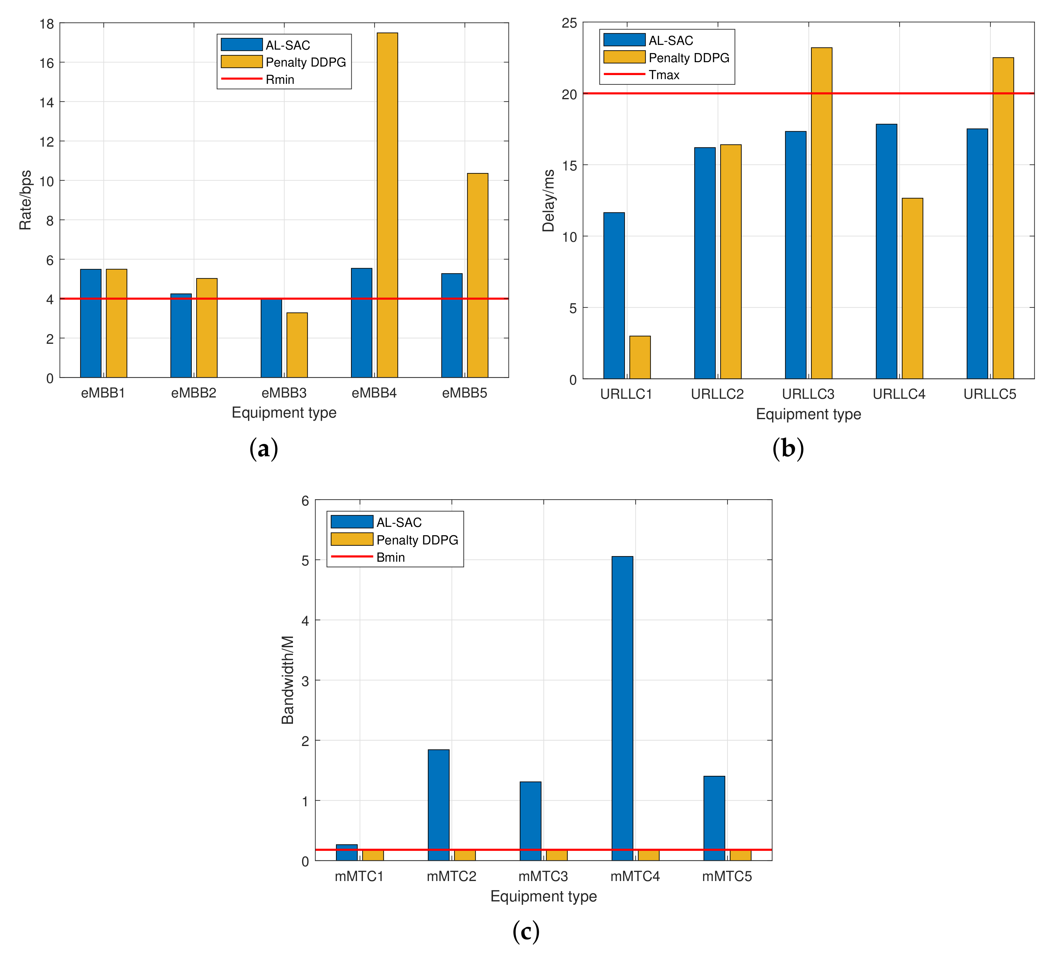
• eMBB slice: The devices served by this network slice require a high transmission rate, such as the device with real-time streaming of high-resolution 4K or 3D video [24]. That is, the transmission rate achieved by these devices has a minimum requirement:

  $$R_n\ge R_0,\forall n\in {\mathcal{N}}_{\mathrm{eM}},$$

  (4)

  where $R_0$ denotes the rate threshold.
• URLLC slice: The devices served by this network slice have a strict requirement on delay, which include the transmission delay, queuing delay, propagation delay, and routing delay [25]. Denoted them by $T_1,T_2,T_3,T_4$, respectively, the end-to-end delay can be calculated as $T_1+T_2+T_3+T_4$. The minimum requirement for wireless transmission delay is as follows:

  $$\frac{L}{R_n}\le T_0,\forall n\in {\mathcal{N}}_{\mathrm{uR}},$$

  (5)

  where L denotes the packet length, and $T_0$ denotes the delay threshold. As mentioned in [26], the achievable rate of a URLLC wireless link, i.e., Equation (4) in [26], can be approximated by the Shannon capacity when the block length is large. For this reason, in this work, we use the Shannon capacity to calculate the link rate and focus on the transmission time independent of the other delay components [27].
• mMTC slice: The devices served by this network slice have no strict rate or latency requirements [27]. Hence, to ensure the basic wireless connection, a minimum bandwidth $B_0$ should be allocated to support the connection. That is,

  $$\sum _{m\in \mathcal{M}}{b}_{nm}\ge B_0,\forall n\in {\mathcal{N}}_{\mathrm{mM}}.$$

  (6)

2.4. Problem Formulation

The aim of network slicing design is maximizing the overall utility achieved by the devices in the system, Firstly, inside each network slice, to achieve fairness among the inner-slice devices, the proportional fairness is utilized as the utility function of each device [28]. That is,

$$U_n=log\left(R_n\right).$$

(7)

More importantly, considering the disparity of throughput in three network slices, weight preference is utilized to balance their contribution to the overall utility [29]. In this work, we use $w_{\mathrm{eM}}$, $w_{\mathrm{uR}}$ and $w_{\mathrm{mM}}$ to denote the weight for the devices in eMBB, URLLC and mMTC slices, respectively.

Hence, we have the following optimization problem, via the BS-device association and bandwidth allocation to maximize the overall system utility:

$$\begin{array}{c}\hfill \underset{b_{nm},x_{nm}}{max}{w}_{\mathrm{eM}}\sum _{n\in {\mathcal{N}}_{\mathrm{eM}}}{U}_n+w_{\mathrm{uR}}\sum _{n\in {\mathcal{N}}_{\mathrm{uR}}}{U}_n+w_{\mathrm{mM}}\sum _{n\in {\mathcal{N}}_{\mathrm{mM}}}{U}_n.\end{array}$$

(8)

$$\begin{array}{c}\hfill \mathrm{s}.\mathrm{t}.\sum _{n\in \mathcal{N}}{x}_{nm}·b_{nm}\le B_m,\forall m,\end{array}$$

(9)

$$\begin{array}{c}\hfill \sum _{m\in \mathcal{M}}{x}_{nm}=1,x_{nm}=\{0,1\},\forall n\in \mathcal{N},\end{array}$$

(10)

$$\begin{array}{c}\hfill R_n\ge R_0,\forall n\in {\mathcal{N}}_{\mathrm{eM}},\end{array}$$

(11)

$$\begin{array}{c}\hfill \sum _{m\in \mathcal{M}}{b}_{nm}\ge B_0,\forall n\in {\mathcal{N}}_{\mathrm{mM}},\end{array}$$

(12)

$$\begin{array}{c}\hfill \frac{L}{R_n}\le T_0,\forall n\in {\mathcal{N}}_{\mathrm{uR}},\end{array}$$

(13)

In addition, (9) represents the bandwidth allocated to the associated users that cannot exceed the overall bandwidth in this BS; (10) indicates that a device only can be associated with one BS at one-time instance; and (11), (12) and (13) represent that the network requirements in each slice introduced above.

In essence, the above problem is a constrained mixed integer problem. In the following, we propose an augmented Lagrangian-based reinforcement learning (RL) with a soft actor–critic (SAC) framework to solve this problem. Then, with the optimal results on the device-BS association and the bandwidth allocated to each device, an extra but simple procedure is needed to complete the slicing details: /(1) Calculate the number of radio resource blocks (RRB) needed for each slice in one BS, and determine the corresponding collection of RRBs. (2) Each BS allocates a subset of the RRBs belonging to the slice to each serving device.

3. Proposed Augmented Lagrangian-Based Reinforcement Learning

In the considered scenario, the agent deploying the proposed algorithm can be the edge server in the 5G architecture. Since the edge server is deployed neighboring the BSs, and with the channel information feedback from the BSs, the proposed algorithm can give the optimal device-BS association and each device’s bandwidth.

In this section, the basic of the augmented Lagrangian method is firstly presented. Then, the hybrid action space, state space, and reward function are defined. Finally, the architecture and workflow of the proposed AL-SAC algorithm are elaborated.

3.1. Preliminary of Augmented Lagrangian Method

The augmented Lagrangian method not only replaces the constrained optimization problem with an unconstrained problem but also introduces a penalty term to accelerate convergence [30]. Given an objective function $f\left(\mathit{x}\right)$ to maximize with parameter $\mathit{x}$ and the constraint functions $c_i\left(\mathit{x}\right)>0$, this optimization problem can be solved by its dual problem as follows:

$$\begin{array}{c}\hfill \underset{\lambda >0}{min}\underset{\mathit{x}}{max}\mathit{L}(\mathit{x},\lambda ,\mu )\triangleq f\left(\mathit{x}\right)+\sum _i{\lambda }_i{c}_i\left(\mathit{x}\right)+\frac{\mu }{2}\sum _i\left|\right|c_i\left(\mathit{x}\right){\left|\right|}^2,\end{array}$$

(14)

where $\lambda$ denotes the Lagrange multiplier vector for the constraints, and $\mu$ denotes the parameter for the penalty term.

Then, the typical solving process alternatively optimizes $\lambda$ and $\mathit{x}$ during iterations. Generally at t-th iteration, ${\lambda }_i^{\left(t\right)}$ is updated according to the rule as

$${\lambda }_i^{\left(t\right)}={\lambda }_i^{\left(t\right)}+{\mu }^{\left(t\right)}{c}_i\left({\mathit{x}}^{\left(t\right)}\right).$$

(15)

Additionally, when the constraint is not satisfied, $\mu$ is enlarged with a scalar.

3.2. Definition of State, Action and Reward in RL

To solve this problem using the framework of RL, in the following, we further define the corresponding state, action spaces, and the reward function in this problem.

3.2.1. State Space

In reinforcement learning, the state space represents the environment observed by an agent. Hence, in our scenario, the wireless environment, i.e., the channel condition between BSs and devices, is defined as the state. Since in the factory, the location of devices are fixed, the channel condition only related to the channel fading gain, that is, the state space, can be expressed as

$${\mathit{s}}^{\left(t\right)}=\{h_{nm}^{\left(t\right)},\forall m,\forall n\}.$$

(16)

Based on the state, we can calculate the SINR by (1), and then the transmission rate and other parameters involved in the optimization problems.

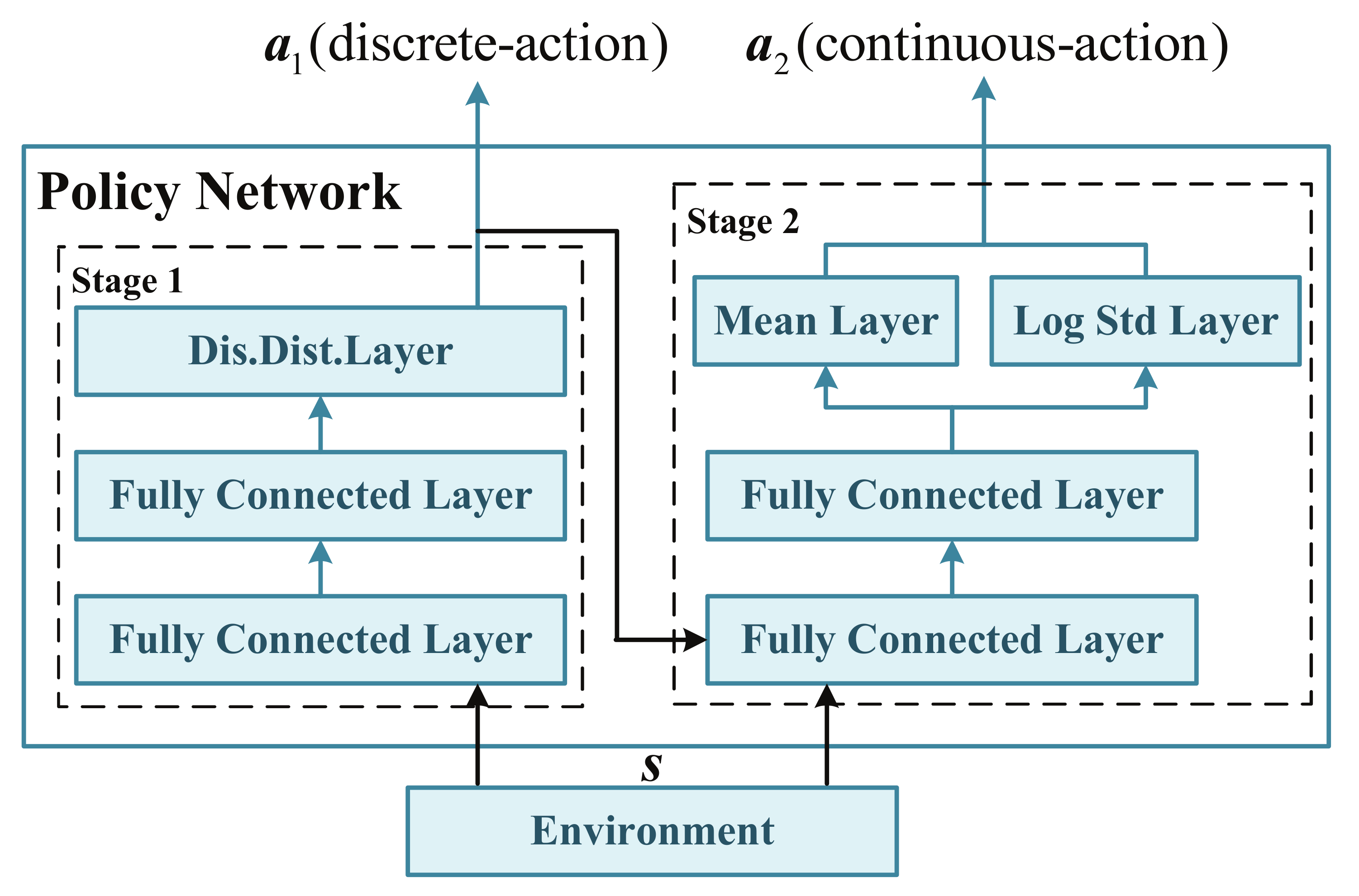
3.2.2. Hybrid Action Space

Considering the discrete and continuous variables involved in problem (8), a hybrid action space is used in this problem. That is, the discrete action,

$${\mathit{a}}_1=\{x_{nm},n\in \mathcal{N},m\in \mathcal{M}\},$$

(17)

which represents the association between devices and BSs; the continuous action

$${\mathit{a}}_2=\{b_{nm},n\in \mathcal{N},m\in \mathcal{M}\},$$

(18)

which represents the bandwidth assigned by BS.

Since a BS only allocates bandwidth resources to its associating devices, we have that only when $x_{mn}=1$, then $b_{mn}>0$. Hence, a hierarchical policy network is designed, where we divide the action selection into two stages to significantly reduce the action space, as illustrated in Figure 2, association action ${\mathit{a}}_1$ is selected at Stage-1 based on the state $\mathit{s}$, and then at Stage-2, bandwidth allocation action ${\mathit{a}}_2$ is chosen based on the set $\{\mathit{s},{\mathit{a}}_1\}$.

In t-th time episode, we denote the action for the whole system as

$${\mathit{a}}^{\left(t\right)}=\{{\mathit{a}}_1^{\left(t\right)},{\mathit{a}}_2^{\left(t\right)}\}.$$

(19)

3.2.3. Reward Function

In (8), we have multiple constraints. For the association constraint, i.e., (10), and the requirement constraints of the devices, i.e., (11)–(13), we directly map the actions to the corresponding ranges. As for bandwidth constraints (9), we consider an augmented Lagrangian method to constrain the total bandwidth since it cannot be handled at the time of action selection.

Motivated by the augmented Lagrangian method, we introduce the penalty into the design of the reward function. In more detail, that is, when the bandwidth constraints of all BS are satisfied, the reward function equals the original weighted overall utility, i.e., (8), which can be calculated as 

$$\begin{array}{c}\hfill r=w_{\mathrm{eM}}\sum _{n\in {\mathcal{N}}_{\mathrm{eM}}}{U}_n+w_{\mathrm{uR}}\sum _{n\in {\mathcal{N}}_{\mathrm{uR}}}{U}_n+w_{\mathrm{mM}}\sum _{n\in {\mathcal{N}}_{\mathrm{mM}}}{U}_n,\end{array}$$

(20)

Otherwise, the reward equals the penalty item similar to the augmented Lagrangian method, that is,

$$\begin{array}{c}\hfill r=\sum _{m\in {\mathcal{M}}^{\prime }}(B_m-G_m),\end{array}$$

(21)

where the set ${\mathcal{M}}^{\prime }$ just involves BSs that do not satisfy the bandwidth constraint, and $G_m={\sum }_{n\in \mathcal{N}}{x}_{nm}{b}_{nm}$ represents the overall bandwidth used in m-th BS. In (21), it means when the total bandwidth constraint is not satisfied, the reward is a negative value related to the exceeded bandwidth.

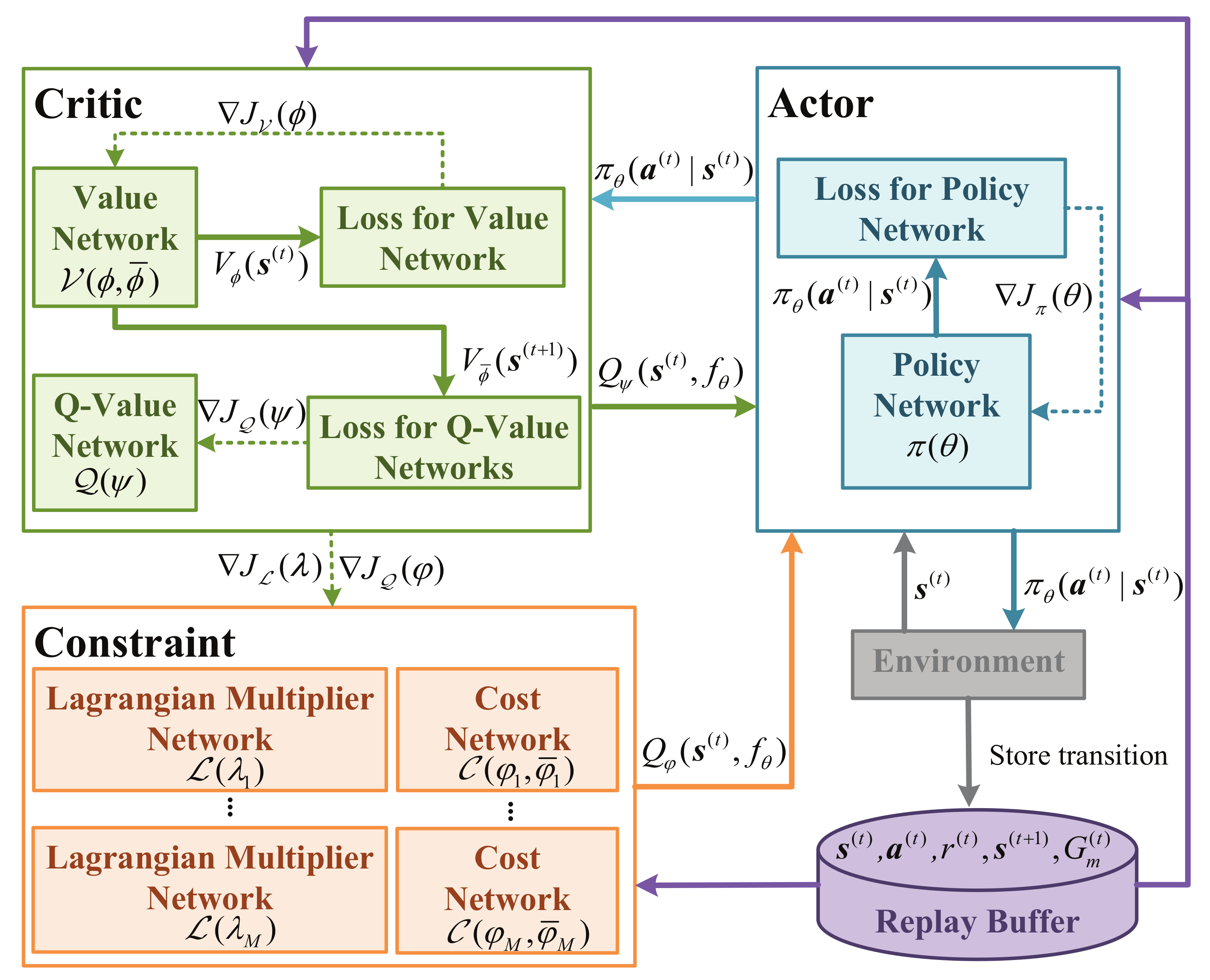
3.3. Proposed AL-SAC Algorithm

The framework of SAC includes the actor and critic parts, which are for policy evaluation and policy improvement, respectively. A policy is the function that returns a feasible action for a state, denoted by $\pi$. That is,

$$\mathit{a}\sim \pi (\times |\mathit{s}).$$

(22)

In SAC, the algorithm aims to find the optimal policy which maximizes the average of the entropy of the policy and the expected reward. That is,

$$\begin{array}{c}\hfill \underset{\pi }{\mathrm{argmax}}\mathbb{E}\left[\sum _{t=0}^T{\gamma }^t\left(r^{\left(t\right)}+\mathit{H}\left(\pi \left({\mathit{a}}^{\left(t\right)}|{\mathit{s}}^{\left(t\right)}\right)\right)\right)\right],\end{array}$$

(23)

where $\gamma (0<\gamma \le 1)$ is the discount factor; $\mathit{H}\left(\pi \right(\mathit{a}\left|\mathit{s}\right))$ denotes the Shannon entropy of policy $\pi$. Considering the hybrid action spaces in our problem, the Shannon entropy for policy $\pi$ involves the entropy calculation of two parts:

$${\mathit{H}}^{{}^{\prime }}\left(\pi \left(\mathit{a}\right|\mathit{s})\right)={\beta }_1\mathit{H}\left(\pi \left({\mathit{a}}_1\right|\mathit{s})\right)+{\beta }_2\mathit{H}\left({\mathit{a}}_2\right|\mathit{s}),$$

(24)

where ${\beta }_1$ and ${\beta }_2$ are the entropy temperatures.

As illustrated in Figure 3, the architecture of the proposed AL-SAC algorithm incorporates a constraint part in addition to the original actor, critic parts, and replay buffer. Specifically,

• Actor part: it deploys a policy network denoted by $\pi$, which generates the policy of device association and bandwidth allocation;
• Critic part: it deploys a value network and a Q-value network, denoted by $\mathcal{V}$ and $\mathcal{Q}$, estimating the value of state and state-action, respectively;
• Constraint part: it deploys Lagrangian multiplier networks and cost networks, denoted by $\mathcal{L}$ and $\mathcal{C}$, estimates the cost value of constraints and adjusting the Lagrangian multipliers accordingly.
• Replay buffer: it is used in DRL to store the tuples, i.e., $\{s^{\left(t\right)},a^{\left(t\right)},r^{\left(t\right)},s^{(t+1)},G_m^{\left(t\right)}\}$, from which the sampled tuples are used in neural network training.

In the following, we describe the updating process of each neural network component in the three parts network.

3.3.1. Value Network $\mathcal{V}$

This network is utilized for estimating the state value and target state value, i.e., $V_{\varphi }\left(\mathit{s}\right)$ and $V_{\overline{\varphi }}\left(\mathit{s}\right)$, where $\varphi$ and $\overline{\varphi }$ are parameters, and $\overline{\varphi }$ is updated by an exponentially moving average of the value network weight [31]. In the learning process, this network is trained by minimizing the squared residual error

$$\begin{array}{c}\hfill J_{\mathcal{V}}\left(\varphi \right)=\mathbb{E}\left[\frac{1}{2}{\left(V_{\varphi }\left({\mathit{s}}^{\left(t\right)}\right)-\mathbb{E}\left[Q_{\psi }\left({\mathit{s}}^{\left(t\right)},{\mathit{a}}^{\left(t\right)}\right)log{\pi }_{\theta }\left({\mathit{a}}^{\left(t\right)}|{\mathit{s}}^{\left(t\right)}\right)\right]\right)}^2\right],\end{array}$$

(25)

Then, the gradient in (25) can be estimated by an unbiased estimator and used in the update of the neural network. That is,

$$\begin{array}{c}\hfill {\nabla }_{\varphi }{J}_{\mathcal{V}}\left(\varphi \right)={\nabla }_{\varphi }{V}_{\varphi }\left({\mathit{s}}^{\left(t\right)}\right)(V_{\varphi }\left({\mathit{s}}^{\left(t\right)}\right)-Q_{\psi }({\mathit{s}}^{\left(t\right)},{\mathit{a}}^{\left(t\right)})+log{\pi }_{\theta }\left({\mathit{a}}^{\left(t\right)}\right|{\mathit{s}}^{\left(t\right)})).\end{array}$$

(26)

3.3.2. Q-Value Network $\mathcal{Q}$

To evaluate the reward function, a Q-value network is deployed to calculate the state-action value for each action, i.e, $Q_{\psi }\left(\mathit{s},\mathit{a}\right)$, where $\psi$ denote the parameter of the neural network. This network is trained by minimizing the soft Bellman residual

$$\begin{array}{c}\hfill J_{\mathcal{Q}}\left(\psi \right)=\mathbb{E}\left[\frac{1}{2}{\left(Q_{\psi }\left({\mathit{s}}^{\left(t\right)},{\mathit{a}}^{\left(t\right)}\right)-\left(r^{\left(t\right)}+\gamma {\mathbb{E}}_{{\mathit{s}}^{(t+1)}}\left[V_{\overline{\varphi }}\left({\mathit{s}}^{(t+1)}\right)\right]\right)\right)}^2\right],\end{array}$$

(27)

where $V_{\overline{\varphi }}\left({\mathit{s}}^{(t+1)}\right)$ is target state value mentioned above to enhance the training stability. Then, this neural network is updated by

$$\begin{array}{c}\hfill {\nabla }_{\psi }{J}_{\mathcal{Q}}\left(\psi \right)={\nabla }_{\psi }{Q}_{\psi }\left({\mathit{s}}^{\left(t\right)},{\mathit{a}}^{\left(t\right)}\right)\left(Q_{\psi }\left({\mathit{s}}^{\left(t\right)},{\mathit{a}}^{\left(t\right)}\right)-r^{\left(t\right)}-\gamma V_{\overline{\varphi }}\left({\mathit{s}}^{(t+1)}\right)\right).\end{array}$$

(28)

3.3.3. Constraint Networks $\mathcal{C}$

Multiple constraint networks are also deployed to estimate the constraints cost expectation for bandwidth allocation. Similar to double deep Q-learning, each constraint network has two separated Q-value networks with parameters ${\phi }_m$ and ${\overline{\phi }}_m$. They are involved in generating the continuous action-state value for m-th BS, i.e., $C_{{\phi }_m}({\mathit{h}}_m^{\left(t\right)},{\mathit{b}}_m^{\left(t\right)})$, where we define the state in m-th BS as 

$${\mathit{h}}_m^{\left(t\right)}=\{h_{nm},\forall n,x_{nm}=1\},$$

(29)

which be utilized for estimating the value allocated bandwidth. Moreover, we also define the continuous action

$${\mathit{b}}_m^{\left(t\right)}=\{b_{nm},\forall n\}.$$

(30)

This network is trained by minimizing the loss. That is,

$$\begin{array}{c}\hfill J_{\mathcal{C}}\left({\phi }_m\right)=\mathbb{E}\left[\frac{1}{2}{\left(C_{{\phi }_m}\left({\mathit{h}}_m^{\left(t\right)},{\mathit{b}}_m^{\left(t\right)}\right)-\left(r^{\left(t\right)}+\gamma C_{{\overline{\phi }}_m}({\mathit{h}}_m^{(t+1)},{\mathit{b}}_m^{(t+1)})\right)\right)}^2\right],\end{array}$$

(31)

They can be updated by

$$\begin{array}{c}\hfill {\nabla }_{{\phi }_m}{J}_{\mathcal{C}}\left({\phi }_m\right)={\nabla }_{{\phi }_m}{C}_{{\phi }_m}\left({\mathit{h}}_m^{\left(t\right)},{\mathit{b}}_m^{\left(t\right)}\right)\left(C_{{\phi }_m}\left({\mathit{h}}_m^{\left(t\right)},{\mathit{b}}_m^{\left(t\right)}\right)-r^{\left(t\right)}-\gamma C_{{\overline{\phi }}_m}({\mathit{h}}_m^{(t+1)},{\mathit{b}}_m^{(t+1)})\right),\end{array}$$

(32)

where $C_{{\overline{\phi }}_m}({\mathit{h}}_m^{(t+1)},{\mathit{b}}_m^{(t+1)})$ is the target action-state value for the training stability, where ${\overline{\phi }}_m$ is periodically updated by copying ${\phi }_m$.

3.3.4. Lagrangian Multiplier Network $\mathcal{L}$

To update Lagrange multiplier $\mathit{\lambda }$ in (15), we also deploy Lagrangian multiplier networks. As mentioned in Section 3.1, we can learn $\lambda$ by minimizing the objective function according to the constraints’ verification. That is,

$$\begin{array}{c}\hfill J\left(\lambda \right)=\mathbb{E}\left[\sum _m{\lambda }_m\left(B_m-G_m\right)\right].\end{array}$$

(33)

3.3.5. Policy Network $\pi$

This network searches the optimal policy according to the estimated values generated by networks in the critic and constraint part. It generates an action based on policy $\pi$ for each state, i.e., ${\pi }_{\theta }(\times |\mathit{s})$, where $\theta$ is the parameter of the policy network. As mentioned earlier, we consider a two-stage action selection. Specifically, the discrete action will be selected first, i.e., the BS connection state will be determined. Then with the corresponding channel state between the device and BS, the bandwidth allocation is determined.

Then, we can update $\pi$ by maximizing the following function

$$\begin{array}{c}\hfill J_{\pi }\left(\theta \right)=\mathbb{E}\left[log\left({\pi }_{\theta }\left({\mathit{a}}^{\left(t\right)}\right|{\mathit{s}}^{\left(t\right)})\right)-Q_{\psi }+\sum _{m\in \mathcal{M}}\left({\lambda }_m{Q}_{{\phi }_m}({\mathit{h}}_m^{\left(t\right)},{\mathit{b}}_m^{\left(t\right)})\right)\right].\end{array}$$

(34)

The gradient of (34) can be approximated by

$$\begin{array}{cc}\hfill {\nabla }_{\theta }{J}_{\pi }\left(\theta \right)=& {\nabla }_{\theta }log{\pi }_{\theta }\left({\mathit{a}}^{\left(t\right)}\right|{\mathit{s}}^{\left(t\right)})+({\nabla }_{{\mathit{a}}^{\left(t\right)}}log{\pi }_{\theta }\left({\mathit{a}}^{\left(t\right)}\right|{\mathit{s}}^{\left(t\right)})-\hfill \\ & {\nabla }_{{\mathit{a}}^{\left(t\right)}}{Q}_{\psi }({\mathit{s}}^{\left(t\right)},{\mathit{a}}^{\left(t\right)})+\sum _{m\in \mathcal{M}}\left({\lambda }_m{Q}_{{\phi }_m}({\mathit{h}}_m^{\left(t\right)},{\mathit{b}}_m^{\left(t\right)})\right)){\nabla }_{\theta }{f}_{\theta }({ϵ}^{\left(t\right)};{\mathit{s}}^{\left(t\right)}),\hfill \end{array}$$

(35)

where ${\mathit{a}}^{\left(t\right)}=f_{\theta }({ϵ}^{\left(t\right)};{\mathit{s}}^{\left(t\right)})$, ${ϵ}^{\left(t\right)}$ is an input vector sampled from Gaussian distribution, and ${\pi }_{\theta }$ is defined implicitly in terms of $f_{\theta }$ [31].

The workflow of the proposed AL-SAC algorithm is summarized in Algorithm 1. Specifically, lines 2–6 illustrate the experience collected from the environment with the current policy, and then the update of the networks is presented in lines 8–18.

Algorithm 1 Augmented Lagrangian-based soft actor–critic (AL-SAC)

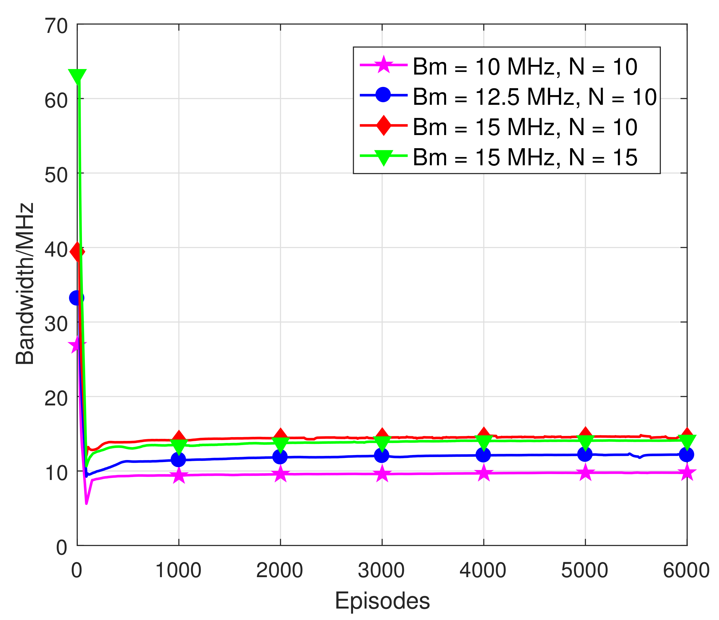
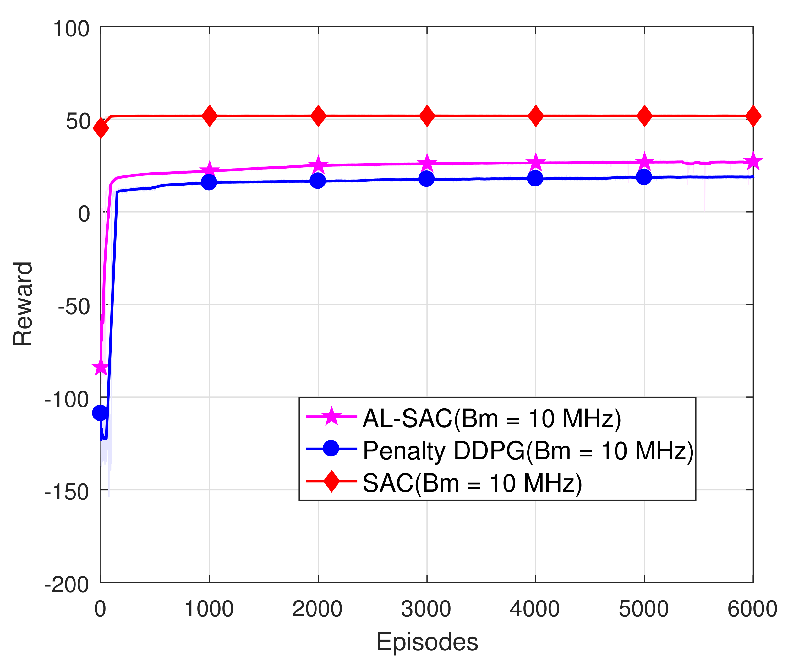
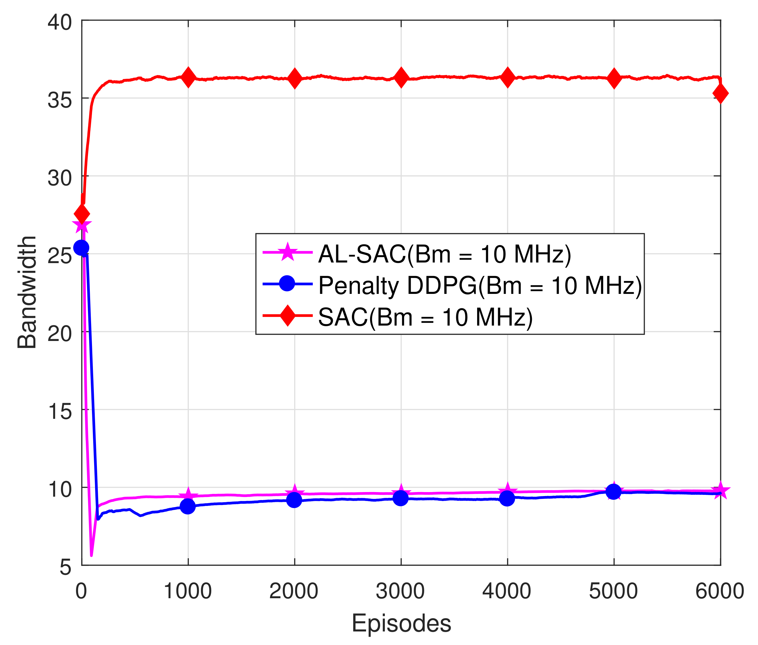
Initialize: Initialize network parameters $\varphi ,\overline{\varphi },\theta ,\psi ,{\phi }_m,m=1,\cdots ,M$, Lagrange multiplier $\mathit{\lambda }$, $\mu$, and replay buffer $\mathcal{D}$. Initialize: Initialize the time episode T, and batch size K. 1: for each time episode $t=1,\cdots ,T$ do 2:     Observe the environment ${\mathit{s}}^{\left(t\right)}$. 3:     Select the action ${\mathit{a}}^{\left(t\right)}\sim {\pi }_{\theta }\left({\mathit{s}}^{\left(t\right)}\right)$. 4:     Calculate total bandwidth allocated in each BS, i.e., $G_m^{\left(t\right)}={\sum }_{n\in \mathcal{N}}{x}_{nm}\times b_{nm}$. 5:     Calculate the reward $r^{\left(t\right)}$ depending on $G_m^{\left(t\right)}$, i.e., (20) or (21). 6:     Update the replay memory buffer $\mathcal{D}\leftarrow \mathcal{D}\cup \{{\mathit{s}}^{\left(t\right)},{\mathit{a}}^{\left(t\right)},r^{\left(t\right)},{\mathit{s}}^{(t+1)},G_m^{\left(t\right)}\}$. 7:     if $t>K$ then 8:         Randomly select a batch of samples $({\mathit{s}}^{\left(t\right)},{\mathit{a}}^{\left(t\right)},r^{\left(t\right)},{\mathit{s}}^{(t+1)})$ from the replay memory buffer $\mathcal{D}$. 9:         Update the value network $\mathcal{V}$ by $\varphi \leftarrow \varphi -{\xi }_V{\nabla }_{\varphi }{J}_V\left(\varphi \right)$. 10:         Update the Q-value network $\mathcal{Q}$ by $\psi \leftarrow \psi -\xi {\nabla }_{\psi }{J}_Q\left(\psi \right)$. 11:         Update the cost networks $\mathcal{C}$ by ${\phi }_m\leftarrow {\phi }_m-{\xi }_m{\nabla }_{\phi }{J}_Q\left({\phi }_m\right)$. 12:         Update the policy network $\pi$ by $\theta \leftarrow \theta -{\xi }_{\pi }{\nabla }_{\theta }{J}_{\pi }\left(\theta \right)$. 13:         Update the Lagrangian multiplier networks $\mathcal{L}$ by ${\mathit{\lambda }}_m\leftarrow {\lambda }_m-\mu {\nabla }_{{\lambda }_m}J\left(\lambda \right)$. 14:         if Constraints not satisfy the requirement then 15:            Enlarge the $\mu$ with a scalar. 16:         end if 17:         Update the parameter $\overline{\varphi }$ by $\overline{\varphi }\leftarrow \delta \varphi +(1-\delta )\overline{\varphi }$. 18:         ${\overline{\phi }}_m$ in cost networks are periodically updated by copying ${\phi }_m$. 19:     end if 20: end for

4. Simulation

In this section, we first test the performance of the proposed AL-SAC algorithm in various scenarios, and also verify the constraints required. Moreover, compare it with other benchmark algorithms, including the original SAC algorithm, and the DDPG algorithm with a penalty item dealing with constraints. In the end, the network service constraints for devices with different weights proportion are shown.

4.1. Parameter Setting

We consider a wireless scenario with multiple BSs and eMBB/URLLC/mMTC devices, where the locations of devices are randomly distributed. The channel fading between a device and BS follows a Rayleigh distribution, varying with time. Combining the distance-based path loss and fading, the channel condition in an episode can be calculated.

In the simulation, the number of BSs is $M=2$, the number of devices in eMBB, URLLC, and mMTC slices are $(3,3,4)$ or $(5,5,5)$. Three different weight designs are considered, that is, $(w_{\mathrm{eM}},w_{\mathrm{UR}},w_{\mathrm{mM}})=(\frac{1}{3},\frac{1}{3},\frac{1}{3})$, $(\frac{2}{3},\frac{1}{6},\frac{1}{6})$, or $(\frac{1}{10},\frac{3}{5},\frac{3}{10})$. Furthermore, the transmission power $P_m$, the path loss exponent $\alpha$ and noise power ${\sigma }^2$ are set as 2 W, $3.09$ and ${10}^{-9}$ W, respectively [32]. For mMTC devices, $B_0=0.18$ MHz, for eMBB devices, $R_0=4$ Mbps, for URLLC devices, $T_0=20$ ms. The available bandwidth for each BS is set as $B_m=10,12.5$, or 15 MHz, the neural networks are trained by the Adam optimizer, and batch size is set as $K=256$. All these simulation parameters are also listed in

Table 1. Settings of parameters.

Parameter	Value
Number of BSs, M	2
Number of devices, N	10 or 15
Number of devices in different slices, $N_{\mathrm{eM}}$, $N_{\mathrm{UR}}$, $N_{\mathrm{mM}}$	3,3,4 or 5,5,5
Transmission power, $P_m$	2 W
Path loss exponent, $\alpha$	3.09
Noise power, ${\sigma }^2$	${10}^{-9}$ W
Minimum bandwidth allocated for mMTC devices, $B_0$	$0.18$ W
Minimum transmission rate for eMBB devices, $R_0$	4 Mbps
Maximum delay for URLLC devices, $T_0$	20 ms
Maximum bandwidth for each BS, $B_m$	$10,12.5,15$ MHz
Weight, $(w_{\mathrm{eM}},w_{\mathrm{UR}},w_{\mathrm{mM}})$	$(\frac{1}{3},\frac{1}{3},\frac{1}{3})$, $(\frac{2}{3},\frac{1}{6},\frac{1}{6})$, $(\frac{1}{10},\frac{3}{5},\frac{3}{10})$.
Batch size, K	256

for clarity.

In Figure 4, we plot the average reward achieved by the proposed AL-SAC algorithm when the maximum bandwidth $B_m=10,12.5$, and 15 MHz available with the number of devices $N=10$ for each BS, respectively, as well as $B=10$ MHz, $N=15$. Firstly, it is observed that in all cases, the proposed AL-SAC algorithm converges, although a slight fluctuation exists when $B_m=15$ MHz, $N=10$. Secondly, we can see that with the growth of available bandwidth, the curve of achieved reward is a little less stable. The reason behind this is that the bandwidth allocation options for multiple devices also increase, i.e., the action space. Thirdly, it can be seen that with the growth of available bandwidth resources, the reward achieved by the proposed algorithm increases apparently, which implies increasing system utilities due to more radio resources being available. Lastly, compared with $B_m=15$ MHz, $N=10$, the proposed AL-SAC algorithm with $B_m=15$ MHz, $N=15$ can reach similar reward but more converge speed because when more devices share the same limited bandwidth resources, the weighted overall utility is not higher. Moreover, the action space for each device reduces when the devices number increases, resulting in more stable performance.

Meanwhile, to verify the proposed algorithm can provide an effective solution to the constrained RL problem, in Figure 5, we also show the bandwidth constraint in the same scenarios as Figure 4. It clearly can be seen that in all the cases, the proposed AL-SAC can meet bandwidth requirements after 100 episodes. This also shows that the proposed algorithm can provide a feasible and effective solution to the constraint optimization problem considered.

In Figure 6 and Figure 7, we compare the performance of the proposed AL-SAC algorithm with two benchmark algorithms: the DDPG algorithm with the penalty involved in the reward function, termed as penalty DDPG [33] and the original soft actor–critic algorithm without constraint handling, termed as SAC [31]. Observe from Figure 6, the SAC algorithm achieves the highest reward, which is much larger than those achieved by AL-SAC and Penalty DDPG. However, from Figure 7, we can see that the overall bandwidth allocated exceeds the maximum bandwidth constraint. Hence, it can be concluded that the high reward achieved by the SAC algorithm is because it cannot handle the constraint of the action sum, resulting in more radio resources being available, i.e., BS cannot satisfy the constraints in (9).

More importantly, comparing the rewards achieved by the proposed AL-SAC and Penalty DDPG, we can see that from Figure 7, both of them satisfy the maximum bandwidth, and the proposed AL-SAC algorithm significantly outperforms the Penalty DDPG algorithm due to the larger reward achieved. The reason behind this is that although Penalty DDPG can meet bandwidth constraints relying on the penalty item in the rewards, the proposed AL-SAC has a strong capability in handling much smaller discrete and continuous action spaces by two stage-design, and the introduction of the constraint part can make the optimizing process more effective. Specifically, the proposed AL-SAC algorithm achieves an improvement of around $42.1\%$ in reward compared to the Penalty DDPG algorithm after 5000 episodes. Moreover, from Figure 7, the overall bandwidth allocated of the proposed AL-SAC algorithm is a little larger than the Penalty DDPG, which is both under the maximum bandwidth $B_m=10$ MHz constraint. It shows that the policy of device association and bandwidth allocation trained by the proposed AL-SAC algorithm are more efficient.

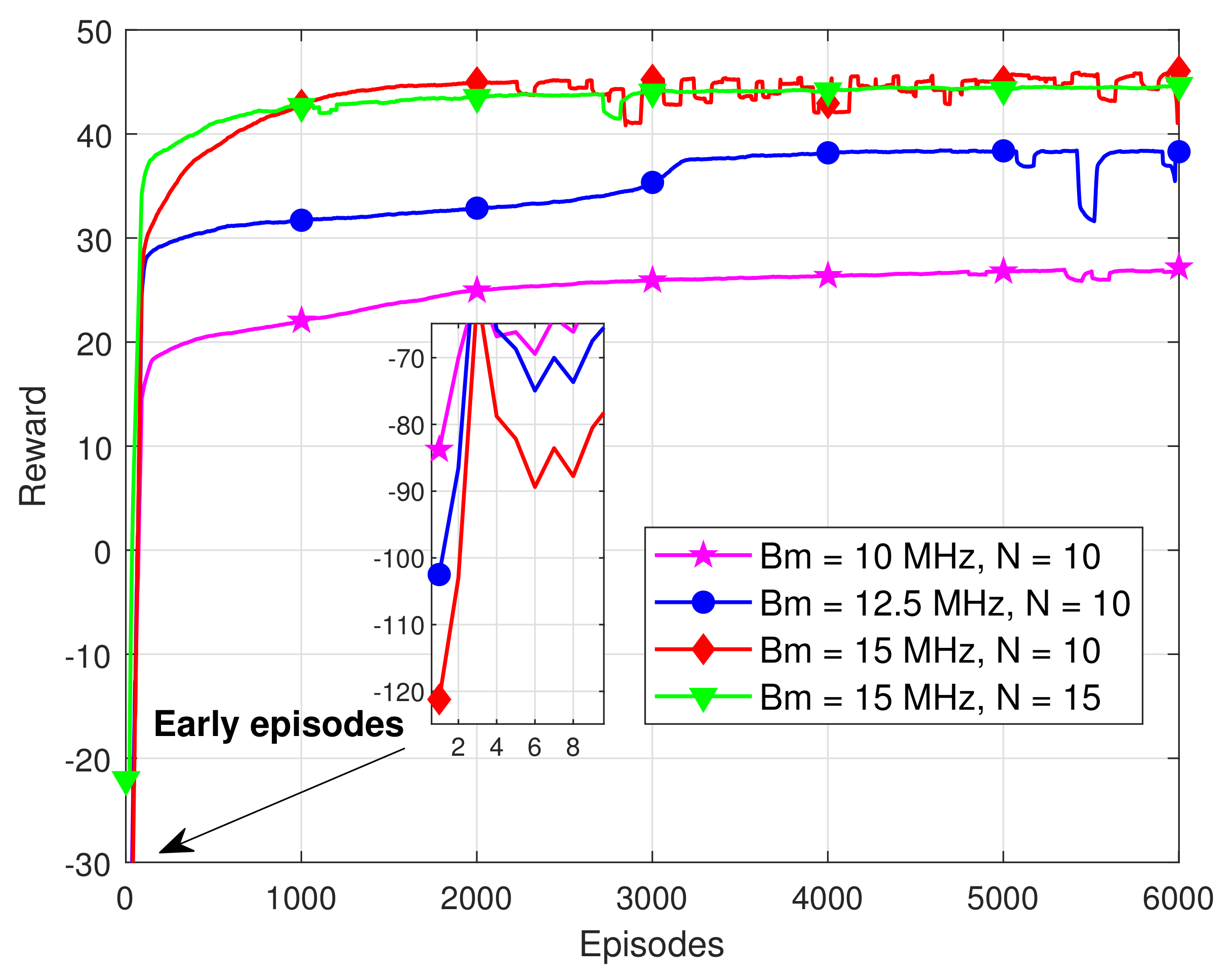
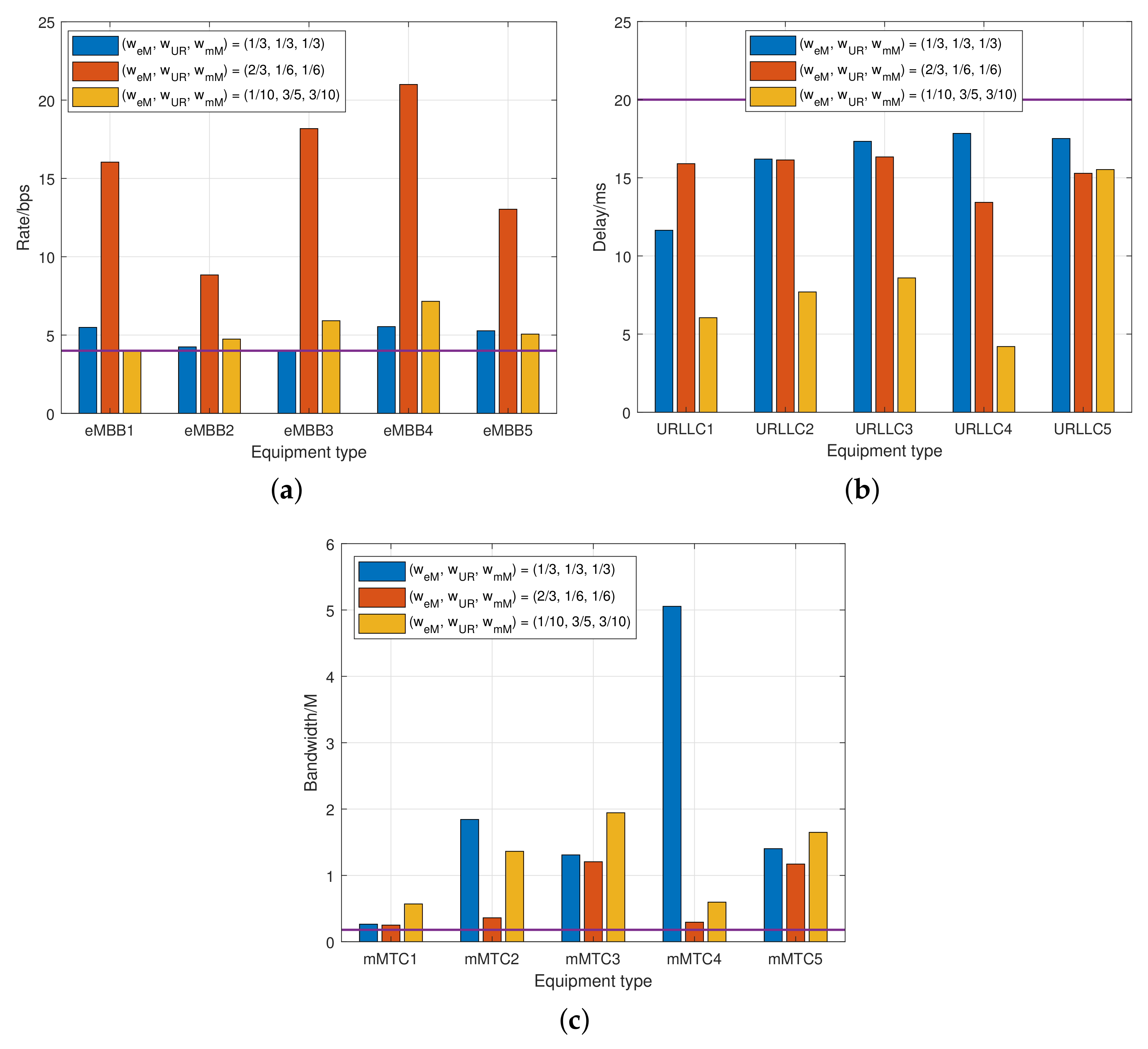
4.2. Results and Analysis

Furthermore, in Figure 8, we tend to verify the performance of each device in different network slices. We consider the scenario of the maximum bandwidth $B_m=10$ MHz; the number of devices $N=15$; the minimum rate requirement for eMBB device $R_0=4$ Mbps; the minimum delay requirement for URLLC device $T_0=20$ ms; and the minimum bandwidth requirement for mMTC device $B_0=0.18$ M. It can be seen from the figure that the proposed AL-SAC algorithm can make all of the devices in various network slices meet their corresponding constraints in three slices, while the Penalty DDPG algorithm cannot. As shown in Figure 8a,b, the device eMBB-3 cannot achieve the required rate, and the devices URLLC-3 and URLLC-5 exceed the maximum delay in (5). Moreover, comparing the transmission rate, delay and bandwidth constraint in the three sub-figures, it can be seen that the network performance achieved by the device in one slice is more even when the proposed AL-SAC algorithm is adopted. This means a better fairness performance is obtained by our proposed AL-SAC algorithm.

To see the results affected by different weights, in Figure 9, we also plot the average reward achieved by the proposed AL-SAC algorithm when weight $(w_{\mathrm{eM}},w_{\mathrm{UR}},w_{\mathrm{mM}})=(\frac{1}{3},\frac{1}{3},\frac{1}{3})$, $(\frac{2}{3},\frac{1}{6},\frac{1}{6})$, and $(\frac{1}{10},\frac{3}{5},\frac{3}{10})$ with the maximum bandwidth $B_m=15$ MHz, $n=10$, respectively. It can be seen that (1) comparing the blue and orange bars in Figure 9a, the total bandwidth allocated to the eMBB slices grows when weight $w_{\mathrm{eM}}$ increases. (2) Comparing the blue and yellow bars in Figure 9b, the overall delay in the URLLC slice reduces when weight $w_{\mathrm{UR}}$ increases. (3) Comparing the yellow bars in Figure 9a,c, the overall bandwidth allocated grows proportionally for devices in mMTC slices when weight $w_{\mathrm{mM}}$. This is because the agent will more attention to the slice with the higher weight.

5. Conclusions

In this paper, we investigated the network slicing problem in IIoT, where the device association and bandwidth allocation for devices in different slices are jointly optimized. By formulating it as a constraint mixed integer nonlinear programming problem with continuous and discrete variables, a Lagrangian-based SAC algorithm is proposed to solve it using DRL. Aiming to maximize the total weighted utility under limited bandwidth resources, cost neural networks and Lagrangian multiplier networks are introduced to update the Lagrangian multipliers and the penalty term is introduced also to the reward function. Moreover, specifically, a novel two-stage actions selection network is presented based on DRL to handle the hybrid actions and decrease the action space simultaneously. Our results verify that the proposed AL-SAC algorithm can effectively meet the constraint and achieve better performance than other benchmark algorithms in terms of average reward and fairness.

References

1. Costanzo, S.; Fajjari, I.; Aitsaadi, N.; Langar, R. Dynamic network slicing for 5G IoT and eMBB services: A new design with prototype and implementation results. In Proceedings of the 2018 3rd Cloudification of the Internet of Things (CIoT), Paris, France, 2–4 July 2018; pp. 1–7. [Google Scholar] [CrossRef]
2. Costanzo, S.; Cherrier, S.; Langar, R. Network slicing orchestration of IoT-BeC3 applications and eMBB services in C-RAN. In Proceedings of the IEEE INFOCOM 2019-IEEE Conference on Computer Communications Workshops (INFOCOM WKSHPS), Paris, France, 29 April–2 May 2019; pp. 975–976. [Google Scholar] [CrossRef]
3. Setayesh, M.; Bahrami, S.; Wong, V.W. Resource Slicing for eMBB and URLLC Services in Radio Access Network Using Hierarchical Deep Learning. IEEE Trans. Wirel. Commun. 2022, 17, 1–11. [Google Scholar] [CrossRef]
4. Popovski, P.; Trillingsgaard, K.F.; Simeone, O.; Durisi, G. 5G Wireless Network Slicing for eMBB, URLLC, and mMTC: A Communication-Theoretic View. IEEE Access 2018, 6, 55765–55779. [Google Scholar] [CrossRef]
5. Chen, W.E.; Fan, X.Y.; Chen, L.X. A CNN-based packet classification of eMBB, mMTC and URLLC applications for 5G. In Proceedings of the 2019 International Conference on Intelligent Computing and its Emerging Applications (ICEA), Tainan, Taiwan, 30 August–1 September 2019; pp. 140–145. [Google Scholar] [CrossRef]
6. Wijethilaka, S.; Liyanage, M. Survey on Network Slicing for Internet of Things Realization in 5G Networks. IEEE Commun. Surv. Tutorials 2021, 23, 957–994. [Google Scholar] [CrossRef]
7. Tang, J.; Shim, B.; Quek, T.Q.S. Service Multiplexing and Revenue Maximization in Sliced C-RAN Incorporated With URLLC and Multicast eMBB. IEEE J. Sel. Areas Commun. 2019, 37, 881–895. [Google Scholar] [CrossRef]
8. Xia, W.; Shen, L. Joint resource allocation using evolutionary algorithms in heterogeneous mobile cloud computing networks. China Commun. 2018, 15, 189–204. [Google Scholar] [CrossRef]
9. Zhang, X.; Zhang, Z.; Yang, L. Learning-Based Resource Allocation in Heterogeneous Ultra Dense Network. IEEE Internet Things J. 2022, 9, 20229–20242. [Google Scholar] [CrossRef]
10. Manogaran, G.; Ngangmeni, J.; Stewart, J.; Rawat, D.B.; Nguyen, T.N. Deep Learning-based Concurrent Resource Allocation for Enhancing Service Response in Secure 6G Network-in-Box Users using IIoT. IEEE Internet Things J. 2021, 9, 1–11. [Google Scholar] [CrossRef]
11. Deng, Z.; Du, Q.; Li, N.; Zhang, Y. RL-based radio Rresource slicing strategy for software-defined satellite networks. In Proceedings of the 2019 IEEE 19th International Conference on Communication Technology (ICCT), Xi’an, China, 16–19 October 2019; pp. 897–901. [Google Scholar] [CrossRef]
12. Kim, Y.; Lim, H. Multi-Agent Reinforcement Learning-Based Resource Management for End-to-End Network Slicing. IEEE Access 2021, 9, 56178–56190. [Google Scholar] [CrossRef]
13. He, Y.; Wang, Y.; Lin, Q.; Li, J. Meta-Hierarchical Reinforcement Learning (MHRL)-Based Dynamic Resource Allocation for Dynamic Vehicular Networks. IEEE Trans. Veh. Technol. 2022, 71, 3495–3506. [Google Scholar] [CrossRef]
14. Alwarafy, A.; Çiftler, B.S.; Abdallah, M.; Hamdi, M.; Al-Dhahir, N. Hierarchical Multi-Agent DRL-Based Framework for Joint Multi-RAT Assignment and Dynamic Resource Allocation in Next-Generation HetNets. IEEE Trans. Netw. Sci. Eng. 2022, 9, 2481–2494. [Google Scholar] [CrossRef]
15. Wang, Y.; Shang, F.; Lei, J. Reliability Optimization for Channel Resource Allocation in Multi-hop Wireless Network: A multi-granularity Deep Reinforcement Learning Approach. IEEE Internet Things J. 2022, 9, 19971–19987. [Google Scholar] [CrossRef]
16. Liu, Y.; Ding, J.; Liu, X. IPO: Interior-point policy optimization under constraints. In Proceedings of the AAAI Conference on Artificial Intelligence, Virtual, 22 Febraury–1 March 2020; Volume 34, pp. 4940–4947. [Google Scholar]
17. Tessler, C.; Mankowitz, D.J.; Mannor, S. Reward constrained policy optimization. arXiv 2018, arXiv:1805.11074. [Google Scholar]
18. Ding, D.; Zhang, K.; Basar, T.; Jovanovic, M. Natural policy gradient primal-dual method for constrained markov decision processes. Adv. Neural Inf. Process. Syst. 2020, 33, 8378–8390. [Google Scholar]
19. Achiam, J.; Held, D.; Tamar, A.; Abbeel, P. Constrained policy optimization. In Proceedings of the International Conference on Machine Learning, PMLR, Sydney, NSW, Australia, 6–11 August 2017; pp. 22–31. [Google Scholar]
20. Schulman, J.; Levine, S.; Abbeel, P.; Jordan, M.; Moritz, P. Trust region policy optimization. In Proceedings of the International Conference on Machine Learning, PMLR, Lille, France, 7–9 July 2015; pp. 1889–1897. [Google Scholar]
21. Yang, T.Y.; Rosca, J.; Narasimhan, K.; Ramadge, P.J. Projection-based constrained policy optimization. arXiv 2020, arXiv:2010.03152. [Google Scholar]
22. Dalal, G.; Dvijotham, K.; Vecerik, M.; Hester, T.; Paduraru, C.; Tassa, Y. Safe exploration in continuous action spaces. arXiv 2018, arXiv:1801.08757. [Google Scholar]
23. Ding, M.; López-Pérez, D.; Chen, Y.; Mao, G.; Lin, Z.; Zomaya, A.Y. Ultra-Dense Networks: A Holistic Analysis of Multi-Piece Path Loss, Antenna Heights, Finite Users and BS Idle Modes. IEEE Trans. Mob. Comput. 2021, 20, 1702–1713. [Google Scholar] [CrossRef]
24. Alsenwi, M.; Tran, N.H.; Bennis, M.; Pandey, S.R.; Bairagi, A.K.; Hong, C.S. Intelligent resource slicing for eMBB and URLLC coexistence in 5G and beyond: A deep reinforcement learning based approach. IEEE Trans. Wirel. Commun. 2021, 20, 4585–4600. [Google Scholar] [CrossRef]
25. Ghanem, W.R.; Jamali, V.; Sun, Y.; Schober, R. Resource allocation for multi-user downlink MISO OFDMA-URLLC systems. IEEE Trans. Commun. 2020, 68, 7184–7200. [Google Scholar] [CrossRef]
26. She, C.; Yang, C.; Quek, T.Q. Joint uplink and downlink resource configuration for ultra-reliable and low-latency communications. IEEE Trans. Commun. 2018, 66, 2266–2280. [Google Scholar] [CrossRef]
27. Suh, K.; Kim, S.; Ahn, Y.; Kim, S.; Ju, H.; Shim, B. Deep Reinforcement Learning-Based Network Slicing for Beyond 5G. IEEE Access 2022, 10, 7384–7395. [Google Scholar] [CrossRef]
28. Liu, Q.; Han, T.; Zhang, N.; Wang, Y. DeepSlicing: Deep reinforcement learning assisted resource allocation for network slicing. In Proceedings of the GLOBECOM 2020–2020 IEEE Global Communications Conference, Virtual, 7–11 December 2020; pp. 1–6. [Google Scholar]
29. Li, M. A Spectrum Allocation Algorithm Based on Proportional Fairness. In Proceedings of the 2020 6th Global Electromagnetic Compatibility Conference (GEMCCON), Xi’an, China, 20–23 October 2020; pp. 1–4. [Google Scholar] [CrossRef]
30. Andreani, R.; Birgin, E.G.; Martínez, J.M.; Schuverdt, M.L. On augmented Lagrangian methods with general lower-level constraints. SIAM J. Optim. 2008, 18, 1286–1309. [Google Scholar] [CrossRef]
31. Haarnoja, T.; Zhou, A.; Abbeel, P.; Levine, S. Soft actor-critic: Off-policy maximum entropy deep reinforcement learning with a stochastic actor. In Proceedings of the International conference on machine learning, PMLR, Jinan, China, 19–21 May 2018; pp. 1861–1870. [Google Scholar]
32. Access, E. Further advancements for E-UTRA physical layer aspects. 3GPP Tech. Specif. TR 2010, 36, V2. [Google Scholar]
33. Bouhamed, O.; Ghazzai, H.; Besbes, H.; Massoud, Y. Autonomous UAV Navigation: A DDPG-Based Deep Reinforcement Learning Approach. In Proceedings of the 2020 IEEE International Symposium on Circuits and Systems (ISCAS), Monterey, CA, USA, 21–25 May 2020; pp. 1–5. [Google Scholar] [CrossRef]
Figure 1. The system model of network slicing. (a) Example of wireless IIoT; (b) the architecture of network slices.
Electronics 11 03385 g001
Figure 2. The structure of two-stage action selection.
Electronics 11 03385 g002
Figure 3. The architecture of proposed AL-SAC algorithm.
Electronics 11 03385 g003
Figure 4. Performance for AL-SAC algorithm with different maximum available bandwidths.
Electronics 11 03385 g004
Figure 5. Total bandwidth allocated for all devices during training process.
Electronics 11 03385 g005
Figure 6. The reward achieved by different algorithms during the training process.
Electronics 11 03385 g006
Figure 7. The total bandwidth allocated by different algorithms.
Electronics 11 03385 g007
Figure 8. Network service constraints for devices in different network slices. (a) The achieved transmission rate of devices in eMBB network slice; (b) the achieved delay of devices in URLLC network slice; (c) the achieved bandwidth of devices in mMTC network slice.
Electronics 11 03385 g008
Figure 9. Network service constraints for devices in different network slices with various weights combination. (a) The achieved transmission rate of devices in eMBB network slice; (b) the achieved delay of devices in URLLC network slice; (c) the achieved bandwidth of devices in mMTC network slice.
Electronics 11 03385 g009