
Multi-Population Enhanced Slime Mould Algorithm and with Application to Postgraduate Employment Stability Prediction


Abstract
:1. Introduction
- (a)
- This paper proposes a novel version of SMA that combines a multi-population strategy called MSMA.
- (b)
- Experiments comparing MSMA with other algorithms are conducted on a benchmark function set. The experimental results demonstrate that the proposed algorithm can better balance the exploitation and exploration capabilities and has better accuracy.
- (c)
- The MSMA algorithm is combined with the support vector machine algorithm to construct a prediction model for the first time, which is called MSMA-SVM. Additionally, the MSMA-SVM model is employed in entrepreneurial intention prediction experiments.
- (d)
- The proposed MSMA in the benchmark function experiment and the MSMA-SVM in entrepreneurial intention prediction demonstrate better performance than their counterparts.
2. Background
2.1. Support Vector Machine
2.2. Slime Mould Algorithm
| Algorithm 1 Pseudo-code of SMA |
| Initialize the parameters popsize, Max_FEs; Initialize the population of slime mould Xi (i = 1, 2, 3, …n); Initialize control parameters z, a; While () Calculate the fitness of slime mould; Sorted in ascending order by fitness; Update ; Calculate the W by Equation (12); For Update Update by Equations (7) and (9); Update by Equations (8) and (10); If rand < z ; Else ; If r < p ; Else ; End If End If End For End While Return |
3. Suggested MSMA
3.1. Multi-Population Structure
3.2. Proposed MSMA
| Algorithm 2 Pseudo-code of MSMA |
| Initialize the parameters popsize, Max_FEs; Initialize the population of slime mould Xi (i = 1, 2, 3, …n); Initialize control parameters z, a; While () Calculate the fitness of slime mould; Sorted in ascending order by fitness; Update ; Calculate the W by Equation (12); For Update Update by Equations (7) and (9); Update by Equations (8) and (10); If rand < z ; Else ; If r < p ; Else ; End If End If End For Perform DNS, SRS, and PDS from multi-population topological structure; End While Return |
3.3. Proposed MSMA-SVM Method
4. Experiments
4.1. Collection of Data
4.2. Experimental Setup
5. Experimental Result
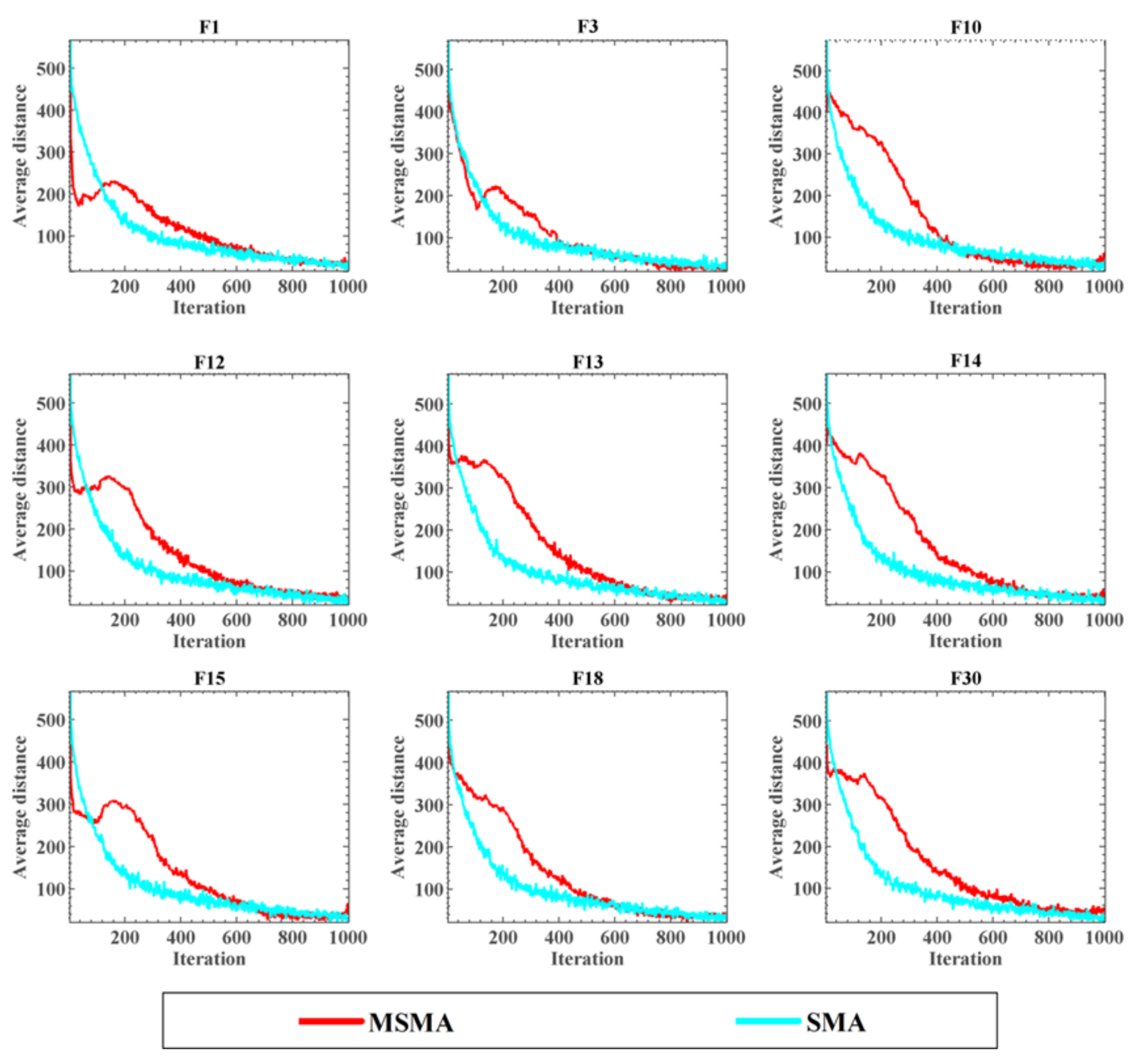
5.1. The Qualitative Analysis of MSMA
5.2. Comparison with Original Methods
5.3. Comparison against Well-Established Algorithms
5.4. Predicting Results of Employment Stability
6. Discussion
7. Conclusions, Limitations, and Future Research
Author Contributions
Funding
Data Availability Statement
Conflicts of Interest
References
- Bharambe, Y.; Mored, N.; Mulchandani, M.; Shankarmani, R.; Shinde, S.G. Assessing employability of students using data mining techniques. In Proceedings of the 2017 International Conference on Advances in Computing, Communications and Informatics (ICACCI), Manipal, Karnataka, India, 13–16 September 2017; pp. 2110–2114. [Google Scholar]
- Li, L.; Zheng, Y.; Sun, X.H.; Wang, F.S. The Application of Decision Tree Algorithm in the Employment Management System. Appl. Mech. Mater. 2014, 543-547, 1639–1642. [Google Scholar] [CrossRef]
- Liu, Y.; Hu, L.; Yan, F.; Zhang, B. Information Gain with Weight Based Decision Tree for the Employment Forecasting of Undergraduates. In Proceedings of the 2013 IEEE International Conference on Green Computing and Communications and IEEE Internet of Things and IEEE Cyber, Physical and Social Computing, Washington, DC, USA, 20–23 August 2013; pp. 2210–2213. [Google Scholar]
- Mahdi, E.; Leiva, V.; Mara’Beh, S.; Martin-Barreiro, C. A New Approach to Predicting Cryptocurrency Returns Based on the Gold Prices with Support Vector Machines during the COVID-19 Pandemic Using Sensor-Related Data. Sensors 2021, 21, 6319. [Google Scholar] [CrossRef] [PubMed]
- Tu, J.; Lin, A.; Chen, H.; Li, Y.; Li, C. Predict the Entrepreneurial Intention of Fresh Graduate Students Based on an Adaptive Support Vector Machine Framework. Math. Probl. Eng. 2019, 2019, 1–16. [Google Scholar] [CrossRef] [Green Version]
- Cuong-Le, T.; Minh, H.-L.; Khatir, S.; Wahab, M.A.; Tran, M.T.; Mirjalili, S. A novel version of Cuckoo search algorithm for solving optimization problems. Expert Syst. Appl. 2021, 186, 115669. [Google Scholar] [CrossRef]
- Abualigah, L.; Elaziz, M.A.; Sumari, P.; Geem, Z.W.; Gandomi, A.H. Reptile Search Algorithm (RSA): A nature-inspired meta-heuristic optimizer. Expert Syst. Appl. 2021, 191, 116158. [Google Scholar] [CrossRef]
- Nadimi-Shahraki, M.H.; Taghian, S.; Mirjalili, S.; Abualigah, L.; Elaziz, M.A.; Oliva, D. EWOA-OPF: Effective Whale Optimization Algorithm to Solve Optimal Power Flow Problem. Electronics 2021, 10, 2975. [Google Scholar] [CrossRef]
- Gandomi, A.H.; Roke, D. A Multi-Objective Evolutionary Framework for Formulation of Nonlinear Structural Systems. IEEE Trans. Ind. Inform. 2021, 1. [Google Scholar] [CrossRef]
- Storn, R.; Price, K. Differential evolution—A simple and efficient heuristic for global optimization over continuous spaces. J. Glob. Optim. 1997, 11, 341–359. [Google Scholar] [CrossRef]
- Li, S.; Chen, H.; Wang, M.; Heidari, A.A.; Mirjalili, S. Slime mould algorithm: A new method for stochastic optimization. Future Gener. Comput. Syst. 2020, 111, 300–323. [Google Scholar] [CrossRef]
- Mirjalili, S.; Mirjalili, S.M.; Lewis, A. Grey Wolf Optimizer. Adv. Eng. Softw. 2014, 69, 46–61. [Google Scholar] [CrossRef] [Green Version]
- Zhao, X.; Zhang, X.; Cai, Z.; Tian, X.; Wang, X.; Huang, Y.; Chen, H.; Hu, L. Chaos enhanced grey wolf optimization wrapped ELM for diagnosis of paraquat-poisoned patients. Comput. Biol. Chem. 2019, 78, 481–490. [Google Scholar] [CrossRef]
- Yang, X.-S. A New Metaheuristic Bat-Inspired Algorithm. In Nature Inspired Cooperative Strategies for Optimization (NICSO 2010). Studies in Computational Intelligence; González, J.R., Pelta, D.A., Cruz, C., Terrazas, G., Krasnogor, N., Eds.; Springer: Berlin/Heidelberg, Germany, 2010; pp. 65–74. [Google Scholar]
- Yang, X.-S. Firefly Algorithms for Multimodal Optimization. In International Symposium on Stochastic Algorithms; Springer: Berlin/Heidelberg, Germany, 2009; pp. 169–178. [Google Scholar]
- Mirjalili, S.; Lewis, A. The Whale Optimization Algorithm. Adv. Eng. Softw. 2016, 95, 51–67. [Google Scholar] [CrossRef]
- Chen, H.; Xu, Y.; Wang, M.; Zhao, X. A balanced whale optimization algorithm for constrained engineering design problems. Appl. Math. Model. 2019, 71, 45–59. [Google Scholar] [CrossRef]
- Mirjalili, S. Moth-flame optimization algorithm: A novel nature-inspired heuristic paradigm. Knowl. Based Syst. 2015, 89, 228–249. [Google Scholar] [CrossRef]
- Xu, Y.; Chen, H.; Luo, J.; Zhang, Q.; Jiao, S.; Zhang, X. Enhanced Moth-flame optimizer with mutation strategy for global optimization. Inf. Sci. 2019, 492, 181–203. [Google Scholar] [CrossRef]
- Xu, Y.; Chen, H.; Heidari, A.A.; Luo, J.; Zhang, Q.; Zhao, X.; Li, C. An efficient chaotic mutative moth-flame-inspired optimizer for global optimization tasks. Expert Syst. Appl. 2019, 129, 135–155. [Google Scholar] [CrossRef]
- Mirjalili, S. SCA: A Sine Cosine Algorithm for solving optimization problems. Knowl. Based Syst. 2016, 96, 120–133. [Google Scholar] [CrossRef]
- Heidari, A.A.; Abbaspour, R.A.; Chen, H. Efficient boosted grey wolf optimizers for global search and kernel extreme learning machine training. Appl. Soft Comput. 2019, 81, 105521. [Google Scholar] [CrossRef]
- Chen, W.-N.; Zhang, J.; Lin, Y.; Chen, N.; Zhan, Z.-H.; Chung, H.; Li, Y.; Shi, Y.-H. Particle Swarm Optimization with an Aging Leader and Challengers. IEEE Trans. Evol. Comput. 2012, 17, 241–258. [Google Scholar] [CrossRef]
- Jia, D.; Zheng, G.; Khan, M.K. An effective memetic differential evolution algorithm based on chaotic local search. Inf. Sci. 2011, 181, 3175–3187. [Google Scholar] [CrossRef]
- Chen, H.; Yang, C.; Heidari, A.A.; Zhao, X. An efficient double adaptive random spare reinforced whale optimization algorithm. Expert Syst. Appl. 2020, 154, 113018. [Google Scholar] [CrossRef]
- Yu, H.; Zhao, N.; Wang, P.; Chen, H.; Li, C. Chaos-enhanced synchronized bat optimizer. Appl. Math. Model. 2020, 77, 1201–1215. [Google Scholar] [CrossRef]
- Lin, A.; Wu, Q.; Heidari, A.A.; Xu, Y.; Chen, H.; Geng, W.; Li, Y.; Li, C. Predicting Intentions of Students for Master Programs Using a Chaos-Induced Sine Cosine-Based Fuzzy K-Nearest Neighbor Classifier. IEEE Access 2019, 7, 67235–67248. [Google Scholar] [CrossRef]
- Heidari, A.A.; Mirjalili, S.; Faris, H.; Aljarah, I.; Mafarja, M.; Chen, H. Harris hawks optimization: Algorithm and applications. Futur. Gener. Comput. Syst. 2019, 97, 849–872. [Google Scholar] [CrossRef]
- Ahmadianfar, I.; Heidari, A.A.; Gandomi, A.H.; Chu, X.; Chen, H. RUN beyond the metaphor: An efficient optimization algorithm based on Runge Kutta method. Expert Syst. Appl. 2021, 181, 115079. [Google Scholar] [CrossRef]
- Tu, J.; Chen, H.; Wang, M.; Gandomi, A.H. The Colony Predation Algorithm. J. Bionic Eng. 2021, 18, 674–710. [Google Scholar] [CrossRef]
- Yang, Y.; Chen, H.; Heidari, A.A.; Gandomi, A.H. Hunger games search: Visions, conception, implementation, deep analysis, perspectives, and towards performance shifts. Expert Syst. Appl. 2021, 177, 114864. [Google Scholar] [CrossRef]
- Zhao, S.; Wang, P.; Heidari, A.A.; Chen, H.; Turabieh, H.; Mafarja, M.; Li, C. Multilevel threshold image segmentation with diffusion association slime mould algorithm and Renyi’s entropy for chronic obstructive pulmonary disease. Comput. Biol. Med. 2021, 134, 104427. [Google Scholar] [CrossRef] [PubMed]
- Liu, L.; Zhao, D.; Yu, F.; Heidari, A.A.; Ru, J.; Chen, H.; Mafarja, M.; Turabieh, H.; Pan, Z. Performance optimization of differential evolution with slime mould algorithm for multilevel breast cancer image segmentation. Comput. Biol. Med. 2021, 138, 104910. [Google Scholar] [CrossRef]
- Yu, C.; Heidari, A.A.; Xue, X.; Zhang, L.; Chen, H.; Chen, W. Boosting quantum rotation gate embedded slime mould algorithm. Expert Syst. Appl. 2021, 181, 115082. [Google Scholar] [CrossRef]
- Liu, Y.; Heidari, A.A.; Ye, X.; Liang, G.; Chen, H.; He, C. Boosting slime mould algorithm for parameter identification of photovoltaic models. Energy 2021, 234, 121164. [Google Scholar] [CrossRef]
- Shi, B.; Ye, H.; Zheng, J.; Zhu, Y.; Heidari, A.A.; Zheng, L.; Chen, H.; Wang, L.; Wu, P. Early Recognition and Discrimination of COVID-19 Severity Using Slime Mould Support Vector Machine for Medical Decision-Making. IEEE Access 2021, 9, 121996–122015. [Google Scholar] [CrossRef]
- Premkumar, M.; Jangir, P.; Sowmya, R.; Alhelou, H.H.; Heidari, A.A.; Chen, H. MOSMA: Multi-Objective Slime Mould Algorithm Based on Elitist Non-Dominated Sorting. IEEE Access 2020, 9, 3229–3248. [Google Scholar] [CrossRef]
- Xia, X.; Gui, L.; Zhan, Z.-H. A multi-swarm particle swarm optimization algorithm based on dynamical topology and purposeful detecting. Appl. Soft Comput. 2018, 67, 126–140. [Google Scholar] [CrossRef]
- Zhang, L.; Zhang, C. Hopf bifurcation analysis of some hyperchaotic systems with time-delay controllers. Kybernetika 2008, 44, 35–42. [Google Scholar]
- Geyer, C.J. Markov Chain Monte Carlo Maximum Likelihood; Interface Foundation of North America: Fairfax Sta, VA, USA, 1991. [Google Scholar]
- Lai, X.; Zhou, Y. Analysis of multiobjective evolutionary algorithms on the biobjective traveling salesman problem (1,2). Multimedia Tools Appl. 2020, 79, 30839–30860. [Google Scholar] [CrossRef]
- Zhang, Y.; Liu, R.; Wang, X.; Chen, H.; Li, C. Boosted binary Harris hawks optimizer and feature selection. Eng. Comput. 2021, 37, 3741–3770. [Google Scholar] [CrossRef]
- Hu, J.; Chen, H.; Heidari, A.A.; Wang, M.; Zhang, X.; Chen, Y.; Pan, Z. Orthogonal learning covariance matrix for defects of grey wolf optimizer: Insights, balance, diversity, and feature selection. Knowl. Based Syst. 2020, 213, 106684. [Google Scholar] [CrossRef]
- Zhang, X.; Xu, Y.; Yu, C.; Heidari, A.A.; Li, S.; Chen, H.; Li, C. Gaussian mutational chaotic fruit fly-built optimization and feature selection. Expert Syst. Appl. 2020, 141, 112976. [Google Scholar] [CrossRef]
- Li, Q.; Chen, H.; Huang, H.; Zhao, X.; Cai, Z.-N.; Tong, C.; Liu, W.; Tian, X. An Enhanced Grey Wolf Optimization Based Feature Selection Wrapped Kernel Extreme Learning Machine for Medical Diagnosis. Comput. Math. Methods Med. 2017, 2017, 1–15. [Google Scholar] [CrossRef]
- Liu, T.; Hu, L.; Ma, C.; Wang, Z.-Y.; Chen, H.-L. A fast approach for detection of erythemato-squamous diseases based on extreme learning machine with maximum relevance minimum redundancy feature selection. Int. J. Syst. Sci. 2013, 46, 919–931. [Google Scholar] [CrossRef]
- Hu, K.; Ye, J.; Fan, E.; Shen, S.; Huang, L.; Pi, J. A novel object tracking algorithm by fusing color and depth information based on single valued neutrosophic cross-entropy. J. Intell. Fuzzy Syst. 2017, 32, 1775–1786. [Google Scholar] [CrossRef] [Green Version]
- Hu, K.; He, W.; Ye, J.; Zhao, L.; Peng, H.; Pi, J. Online Visual Tracking of Weighted Multiple Instance Learning via Neutrosophic Similarity-Based Objectness Estimation. Symmetry 2019, 11, 832. [Google Scholar] [CrossRef] [Green Version]
- Chen, M.-R.; Zeng, G.-Q.; Lu, K.-D.; Weng, J. A Two-Layer Nonlinear Combination Method for Short-Term Wind Speed Prediction Based on ELM, ENN, and LSTM. IEEE Internet Things J. 2019, 6, 6997–7010. [Google Scholar] [CrossRef]
- Zeng, G.-Q.; Lu, K.; Dai, Y.-X.; Zhang, Z.; Chen, M.-R.; Zheng, C.-W.; Wu, D.; Peng, W.-W. Binary-coded extremal optimization for the design of PID controllers. Neurocomputing 2014, 138, 180–188. [Google Scholar] [CrossRef]
- Zeng, G.-Q.; Chen, J.; Dai, Y.-X.; Li, L.-M.; Zheng, C.-W.; Chen, M.-R. Design of fractional order PID controller for automatic regulator voltage system based on multi-objective extremal optimization. Neurocomputing 2015, 160, 173–184. [Google Scholar] [CrossRef]
- Zeng, G.-Q.; Xie, X.-Q.; Chen, M.-R.; Weng, J. Adaptive population extremal optimization-based PID neural network for multivariable nonlinear control systems. Swarm Evol. Comput. 2019, 44, 320–334. [Google Scholar] [CrossRef]
- Zhao, D.; Liu, L.; Yu, F.; Heidari, A.A.; Wang, M.; Liang, G.; Muhammad, K.; Chen, H. Chaotic random spare ant colony optimization for multi-threshold image segmentation of 2D Kapur entropy. Knowl. Based Syst. 2021, 216, 106510. [Google Scholar] [CrossRef]
- Zhao, D.; Liu, L.; Yu, F.; Heidari, A.A.; Wang, M.; Oliva, D.; Muhammad, K.; Chen, H. Ant colony optimization with horizontal and vertical crossover search: Fundamental visions for multi-threshold image segmentation. Expert Syst. Appl. 2020, 167, 114122. [Google Scholar] [CrossRef]
- Zeng, G.-Q.; Lu, Y.-Z.; Mao, W.-J. Modified extremal optimization for the hard maximum satisfiability problem. J. Zhejiang Univ. Sci. C 2011, 12, 589–596. [Google Scholar] [CrossRef]
- Zeng, G.; Zheng, C.; Zhang, Z.; Lu, Y. An Backbone Guided Extremal Optimization Method for Solving the Hard Maximum Satisfiability Problem. Int. J. Innov. Comput. Inf. Control. 2012, 8, 8355–8366. [Google Scholar] [CrossRef] [Green Version]
- Shen, L.; Chen, H.; Yu, Z.; Kang, W.; Zhang, B.; Li, H.; Yang, B.; Liu, D. Evolving support vector machines using fruit fly optimization for medical data classification. Knowl. Based Syst. 2016, 96, 61–75. [Google Scholar] [CrossRef]
- Wang, M.; Chen, H.; Yang, B.; Zhao, X.; Hu, L.; Cai, Z.; Huang, H.; Tong, C. Toward an optimal kernel extreme learning machine using a chaotic moth-flame optimization strategy with applications in medical diagnoses. Neurocomputing 2017, 267, 69–84. [Google Scholar] [CrossRef]
- Wang, M.; Chen, H. Chaotic multi-swarm whale optimizer boosted support vector machine for medical diagnosis. Appl. Soft Comput. 2020, 88, 105946. [Google Scholar] [CrossRef]
- Deng, W.; Xu, J.; Zhao, H.; Song, Y. A Novel Gate Resource Allocation Method Using Improved PSO-Based QEA. IEEE Trans. Intell. Transp. Syst. 2020, PP, 1–9. [Google Scholar] [CrossRef]
- Deng, W.; Xu, J.; Song, Y.; Zhao, H. An Effective Improved Co-evolution Ant Colony Optimization Algorithm with Multi-Strategies and Its Application. Int. J. Bio-Inspired Comput. 2020, 16, 158–170. [Google Scholar] [CrossRef]
- Deng, W.; Liu, H.; Xu, J.; Zhao, H.; Song, Y. An Improved Quantum-Inspired Differential Evolution Algorithm for Deep Belief Network. IEEE Trans. Instrum. Meas. 2020, 69, 7319–7327. [Google Scholar] [CrossRef]
- Zhao, H.; Liu, H.; Xu, J.; Deng, W. Performance Prediction Using High-Order Differential Mathematical Morphology Gradient Spectrum Entropy and Extreme Learning Machine. IEEE Trans. Instrum. Meas. 2020, 69, 4165–4172. [Google Scholar] [CrossRef]
- Zhao, X.; Li, D.; Yang, B.; Ma, C.; Zhu, Y.; Chen, H. Feature selection based on improved ant colony optimization for online detection of foreign fiber in cotton. Appl. Soft Comput. 2014, 24, 585–596. [Google Scholar] [CrossRef]
- Zhao, X.; Li, D.; Yang, B.; Chen, H.; Yang, X.; Yu, C.; Liu, S. A two-stage feature selection method with its application. Comput. Electr. Eng. 2015, 47, 114–125. [Google Scholar] [CrossRef]
- Zhang, X.; Du, K.-J.; Zhan, Z.-H.; Kwong, S.; Gu, T.-L.; Zhang, J. Cooperative Coevolutionary Bare-Bones Particle Swarm Optimization With Function Independent Decomposition for Large-Scale Supply Chain Network Design With Uncertainties. IEEE Trans. Cybern. 2019, 50, 4454–4468. [Google Scholar] [CrossRef]
- Chen, Z.-G.; Zhan, Z.-H.; Lin, Y.; Gong, Y.-J.; Gu, T.-L.; Zhao, F.; Yuan, H.-Q.; Chen, X.; Li, Q.; Zhang, J. Multiobjective Cloud Workflow Scheduling: A Multiple Populations Ant Colony System Approach. IEEE Trans. Cybern. 2019, 49, 2912–2926. [Google Scholar] [CrossRef]
- Wang, Z.-J.; Zhan, Z.-H.; Yu, W.-J.; Lin, Y.; Zhang, J.; Gu, T.-L.; Zhang, J. Dynamic Group Learning Distributed Particle Swarm Optimization for Large-Scale Optimization and Its Application in Cloud Workflow Scheduling. IEEE Trans. Cybern. 2020, 50, 2715–2729. [Google Scholar] [CrossRef]
- Yang, Z.; Li, K.; Guo, Y.; Ma, H.; Zheng, M. Compact real-valued teaching-learning based optimization with the applications to neural network training. Knowl. Based Syst. 2018, 159, 51–62. [Google Scholar] [CrossRef]
- Zhou, S.-Z.; Zhan, Z.-H.; Chen, Z.-G.; Kwong, S.; Zhang, J. A Multi-Objective Ant Colony System Algorithm for Airline Crew Rostering Problem with Fairness and Satisfaction. IEEE Trans. Intell. Transp. Syst. 2020, 22, 6784–6798. [Google Scholar] [CrossRef]
- Liang, D.; Zhan, Z.-H.; Zhang, Y.; Zhang, J. An Efficient Ant Colony System Approach for New Energy Vehicle Dispatch Problem. IEEE Trans. Intell. Transp. Syst. 2019, 21, 4784–4797. [Google Scholar] [CrossRef]
- Liang, J.J.; Qu, B.Y.; Suganthan, P.N. Problem definitions and evaluation criteria for the CEC 2017 special session and competition on single objective real-parameter numerical optimization. Tech. Rep. 2016, 635, 490. [Google Scholar]
- Derrac, J.; García, S.; Molina, D.; Herrera, F. A practical tutorial on the use of nonparametric statistical tests as a methodology for comparing evolutionary and swarm intelligence algorithms. Swarm Evol. Comput. 2011, 1, 3–18. [Google Scholar] [CrossRef]
- García, S.; Fernández, A.; Luengo, J.; Herrera, F. Advanced nonparametric tests for multiple comparisons in the design of experiments in computational intelligence and data mining: Experimental analysis of power. Inf. Sci. 2010, 180, 2044–2064. [Google Scholar] [CrossRef]
- Hua, Y.; Liu, Q.; Hao, K.; Jin, Y. A Survey of Evolutionary Algorithms for Multi-Objective Optimization Problems with Irregular Pareto Fronts. IEEE/CAA J. Autom. Sin. 2021, 8, 303–318. [Google Scholar] [CrossRef]
- Zhang, W.; Hou, W.; Li, C.; Yang, W.; Gen, M. Multidirection Update-Based Multiobjective Particle Swarm Optimization for Mixed No-Idle Flow-Shop Scheduling Problem. Complex Syst. Model. Simul. 2021, 1, 176–197. [Google Scholar] [CrossRef]
- Gu, Z.-M.; Wang, G.-G. Improving NSGA-III algorithms with information feedback models for large-scale many-objective optimization. Futur. Gener. Comput. Syst. 2020, 107, 49–69. [Google Scholar] [CrossRef]
- Yi, J.-H.; Deb, S.; Dong, J.; Alavi, A.H.; Wang, G.-G. An improved NSGA-III algorithm with adaptive mutation operator for Big Data optimization problems. Futur. Gener. Comput. Syst. 2018, 88, 571–585. [Google Scholar] [CrossRef]
- Zhao, F.; Di, S.; Cao, J.; Tang, J. Jonrinaldi A Novel Cooperative Multi-Stage Hyper-Heuristic for Combination Optimization Problems. Complex Syst. Model. Simul. 2021, 1, 91–108. [Google Scholar] [CrossRef]
- Hu, Z.; Wang, J.; Zhang, C.; Luo, Z.; Luo, X.; Xiao, L.; Shi, J. Uncertainty Modeling for Multi center Autism Spectrum Disorder Classification Using Takagi-Sugeno-Kang Fuzzy Systems. IEEE Trans. Cogn. Dev. Syst. 2021, 1. [Google Scholar] [CrossRef]
- Chen, C.Z.; Wu, Q.; Li, Z.Y.; Xiao, L.; Hu, Z.Y. Diagnosis of Alzheimer’s disease based on Deeply-Fused Nets. Comb. Chem. High Throughput Screen. 2020, 24, 781–789. [Google Scholar] [CrossRef]
- Fei, X.; Wang, J.; Ying, S.; Hu, Z.; Shi, J. Projective parameter transfer based sparse multiple empirical kernel learning Machine for diagnosis of brain disease. Neurocomputing 2020, 413, 271–283. [Google Scholar] [CrossRef]
- Saber, A.; Sakr, M.; Abo-Seida, O.M.; Keshk, A.; Chen, H. A Novel Deep-Learning Model for Automatic Detection and Classification of Breast Cancer Using the Transfer-Learning Technique. IEEE Access 2021, 9, 71194–71209. [Google Scholar] [CrossRef]
- Wu, Z.; Li, G.; Shen, S.; Lian, X.; Chen, E.; Xu, G. Constructing dummy query sequences to protect location privacy and query privacy in location-based services. World Wide Web 2021, 24, 25–49. [Google Scholar] [CrossRef]
- Wu, Z.; Wang, R.; Li, Q.; Lian, X.; Xu, G.; Chen, E.; Liu, X. A Location Privacy-Preserving System Based on Query Range Cover-Up or Location-Based Services. IEEE Trans. Veh. Technol. 2020, 69, 5244–5254. [Google Scholar] [CrossRef]
- Xue, X.; Zhou, D.; Chen, F.; Yu, X.; Feng, Z.; Duan, Y.; Meng, L.; Zhang, M. From SOA to VOA: A Shift in Understanding the Operation and Evolution of Service Ecosystem. IEEE Trans. Serv. Comput. 2021, 1. [Google Scholar] [CrossRef]
- Zhang, L.; Zou, Y.; Wang, W.; Jin, Z.; Su, Y.; Chen, H. Resource allocation and trust computing for blockchain-enabled edge computing system. Comput. Secur. 2021, 105, 102249. [Google Scholar] [CrossRef]
- Zhang, L.; Zhang, Z.; Wang, W.; Waqas, R.; Zhao, C.; Kim, S.; Chen, H. A Covert Communication Method Using Special Bitcoin Addresses Generated by Vanitygen. Comput. Mater. Contin. 2020, 65, 597–616. [Google Scholar]
- Zhang, L.; Zhang, Z.; Wang, W.; Jin, Z.; Su, Y.; Chen, H. Research on a Covert Communication Model Realized by Using Smart Contracts in Blockchain Environment. IEEE Syst. J. 2021, 1–12. [Google Scholar] [CrossRef]
- Qiu, S.; Hao, Z.; Wang, Z.; Liu, L.; Liu, J.; Zhao, H.; Fortino, G. Sensor Combination Selection Strategy for Kayak Cycle Phase Segmentation Based on Body Sensor Networks. IEEE Internet Things J. 2021, 1. [Google Scholar] [CrossRef]
- Zhang, X.; Wang, T.; Wang, J.; Tang, G.; Zhao, L. Pyramid Channel-based Feature Attention Network for image dehazing. Comput. Vis. Image Underst. 2020, 197–198, 103003. [Google Scholar] [CrossRef]
- Liu, H.; Li, X.; Zhang, S.; Tian, Q. Adaptive Hashing With Sparse Matrix Factorization. IEEE Trans. Neural Networks Learn. Syst. 2019, 31, 4318–4329. [Google Scholar] [CrossRef]
- Wu, Z.; Li, R.; Zhou, Z.; Guo, J.; Jiang, J.; Su, X. A user sensitive subject protection approach for book search service. J. Assoc. Inf. Sci. Technol. 2020, 71, 183–195. [Google Scholar] [CrossRef]
- Wu, Z.; Shen, S.; Lian, X.; Su, X.; Chen, E. A dummy-based user privacy protection approach for text information retrieval. Knowl. Based Syst. 2020, 195, 105679. [Google Scholar] [CrossRef]
- Wu, Z.; Shen, S.; Zhou, H.; Li, H.; Lu, C.; Zou, D. An effective approach for the protection of user commodity viewing privacy in e-commerce website. Knowl. Based Syst. 2021, 220, 106952. [Google Scholar] [CrossRef]
- Liu, H.; Liu, L.; Le, T.D.; Lee, I.; Sun, S.; Li, J. Nonparametric Sparse Matrix Decomposition for Cross-View Dimensionality Reduction. IEEE Trans. Multimedia 2017, 19, 1848–1859. [Google Scholar] [CrossRef]
- Qiu, S.; Zhao, H.; Jiang, N.; Wu, D.; Song, G.; Zhao, H.; Wang, Z. Sensor network oriented human motion capture via wearable intelligent system. Int. J. Intell. Syst. 2021, 37, 1646–1673. [Google Scholar] [CrossRef]
- Liu, P.; Gao, H. A novel green supplier selection method based on the interval type-2 fuzzy prioritized choquet bonferroni means. IEEE/CAA J. Autom. Sin. 2020, 1–17. [Google Scholar] [CrossRef]
- Han, X.; Han, Y.; Chen, Q.; Li, J.; Sang, H.; Liu, Y.; Pan, Q.; Nojima, Y. Distributed Flow Shop Scheduling with Sequence-Dependent Setup Times Using an Improved Iterated Greedy Algorithm. Complex Syst. Model. Simul. 2021, 1, 198–217. [Google Scholar] [CrossRef]
- Gao, D.; Wang, G.-G.; Pedrycz, W. Solving Fuzzy Job-Shop Scheduling Problem Using DE Algorithm Improved by a Selection Mechanism. IEEE Trans. Fuzzy Syst. 2020, 28, 3265–3275. [Google Scholar] [CrossRef]
- Cao, X.; Cao, T.; Gao, F.; Guan, X. Risk-Averse Storage Planning for Improving RES Hosting Capacity Under Uncertain Siting Choices. IEEE Trans. Sustain. Energy 2021, 12, 1984–1995. [Google Scholar] [CrossRef]
- Cao, X.; Wang, J.; Wang, J.; Zeng, B. A Risk-Averse Conic Model for Networked Microgrids Planning with Reconfiguration and Reorganizations. IEEE Trans. Smart Grid 2020, 11, 696–709. [Google Scholar] [CrossRef]
- Ramadan, A.; Kamel, S.; Taha, I.B.M.; Tostado-Véliz, M. Parameter Estimation of Modified Double-Diode and Triple-Diode Photovoltaic Models Based on Wild Horse Optimizer. Electronics 2021, 10, 2308. [Google Scholar] [CrossRef]
- Liu, Y.; Ran, J.; Hu, H.; Tang, B. Energy-Efficient Virtual Network Function Reconfiguration Strategy Based on Short-Term Resources Requirement Prediction. Electronics 2021, 10, 2287. [Google Scholar] [CrossRef]
- Shafqat, W.; Malik, S.; Lee, K.-T.; Kim, D.-H. PSO Based Optimized Ensemble Learning and Feature Selection Approach for Efficient Energy Forecast. Electronics 2021, 10, 2188. [Google Scholar] [CrossRef]
- Choi, H.-T.; Hong, B.-W. Unsupervised Object Segmentation Based on Bi-Partitioning Image Model Integrated with Classification. Electronics 2021, 10, 2296. [Google Scholar] [CrossRef]
- Saeed, U.; Shah, S.Y.; Shah, S.A.; Ahmad, J.; Alotaibi, A.A.; Althobaiti, T.; Ramzan, N.; Alomainy, A.; Abbasi, Q.H. Discrete Human Activity Recognition and Fall Detection by Combining FMCW RADAR Data of Heterogeneous Environments for Independent Assistive Living. Electronincs 2021, 10, 2237. [Google Scholar] [CrossRef]


| ID | Attribute | Description |
|---|---|---|
| F1 | gender | Male and female students are marked as 1 and 2, respectively. |
| F2 | political status (PS) | There are four categories: Communist Party members, reserve party members, Communist Youth League members, and the masses, denoted by 1, 2, 3, and 13, respectively. |
| F3 | division of liberal arts and science (DLS) | Liberal arts and sciences are indicated by 1 and 2. |
| F4 | years of schooling (YS) | The 3-year and 4-year academic terms are indicated by 3 and 4. |
| F5 | students with difficulties (SWD) | There are four categories: non-difficult students, employment difficulties, family financial difficulties, and dual employment and family financial difficulties, which are indicated by 0, 1, 2, and 3, respectively. |
| F6 | student origin (OS) | There are three categories: urban, township, and rural, denoted by 1, 2, and 3, respectively. |
| F7 | career development after graduation (CDG) | There are three categories of direct employment, pending employment, and further education, which are indicated by 1, 2, and 3, respectively. |
| F8 | unit of first employment (UFE) | Employment pending is indicated by 0. State organizations are indicated by 10, scientific research institutions are indicated by 20, higher education institutions are indicated by 21, middle and junior high education institutions are indicated by 22, health and medical institutions are indicated by 23, other institutions are indicated by 29, state-owned enterprises are indicated by 31, foreign-funded enterprises are indicated by 32, private enterprises are indicated by 39, troops are indicated by 40, rural organizations are indicated by 55, and self-employment is indicated by 99. |
| F9 | location of first employment (LFE) | Employment pending is indicated by 0, sub-provincial and above large cities by 1, prefecture-level cities by 2, and counties and villages by 3. |
| F10 | position of first employment (PFE) | Employment pending is represented by 0, civil servants by 10, doctoral students and researchers by 11, engineers and technicians by 13, teaching staff by 24, professional and technical staff by 29, commercial service staff and clerks by 30, and military personnel by 80. |
| F11 | degree of specialty relevance of first employment (DSRFE) | The correlation between major and job is measured, and the higher the percentage, the higher the correlation. |
| F12 | monthly salary of first employment (MSFE) | Used to measure the average monthly salary earned, with higher values indicating higher salary levels. |
| F13 | status of current employment (SCE) | Three years after graduation, the employment status is represented by 1, 2, and 3 for the categories of employment, pending employment, and further education, respectively. |
| F14 | employment change (EC) | When comparing the employment units three years after graduation with initial employment units, no change is indicated by 0 and any change is indicated by 1. |
| F15 | unit of current employment (UCE) | The nature of the employment unit three years after graduation is expressed in the same way as the nature of initial employment unit in F8. |
| F16 | location of current employment (LCE) | The type employment location three years after graduation is expressed in the same way as the initial employment location in F9. |
| F17 | change in place of employment (CPE) | Used to measure the changes in employment location from the initial employment location three years after graduation and is expressed as the difference between F16 current employment location type and F9 initial employment location type, and the larger the absolute value of the difference, the larger the change in employment location. |
| F18 | position of current employment (PCE) | The job type three years after graduation is expressed in the same way as the initial employment job type in F10. |
| F19 | specialty relevance of current employment (SRCE) | The professional relevance of employment three years after graduation is expressed in the same way as the initial employment job type in F11. |
| F20 | monthly salary of current employment (MSCE) | The monthly salary level three years after graduation is expressed in the same way as the monthly salary level during initial employment in F12. |
| F21 | salary difference (SD) | Used to measure the changes in the graduates’ monthly salary in their current employment and initial employment, i.e., the difference between F20 monthly salary level in current employment and F12 monthly salary level in initial employment, with a larger value indicating a larger increase in monthly salary. |
| F22 | grade point average (GPA) | Used to assess the how much the postgraduate students learned while they were in school and is the average of the final grades of courses taken by graduate students, with higher averages indicating higher quality learning. |
| F23 | scores of teaching practice (STP) | A method used to assess the quality of learning in postgraduate teaching practice sessions, with excellent, good, moderate, pass, and fail expressed as 1, 2, 3, 4, and 5, respectively. |
| F24 | scores of social practices (SSP) | A method used to assess how much the postgraduate students learned in social practice sessions, with excellent, good, moderate, pass, and fail expressed as 1, 2, 3, 4, and 5, respectively. |
| F25 | scores of academic reports (SAR) | A method used to assess how the must the postgraduate students learned during academic reporting sessions, with excellent, good, moderate, pass, and fail expressed as 1, 2, 3, 4, and 5, respectively. |
| F26 | scores of graduation thesis (SGT) | A method used to assess the how much the postgraduate students learned during the thesis sessions, with excellent, good, moderate, pass, and fail expressed as 1, 2, 3, 4, and 5, respectively. |
| MSMA | SMA | DE | GWO | BA | FA | WOA | MFO | SCA | ||
|---|---|---|---|---|---|---|---|---|---|---|
| F1 | Avg | 1.31 × 10² | 8.03 × 10³ | 1.79 × 10³ | 2.24 × 10⁹ | 5.72 × 10⁵ | 1.55 × 10+10 | 2.36 × 10⁷ | 9.38 × 10⁹ | 1.41 × 10+10 |
| Std | 1.68 × 10² | 7.18 × 10³ | 2.96 × 10³ | 1.68 × 10⁹ | 3.78 × 10⁵ | 1.58 × 10⁹ | 1.86 × 10⁷ | 7.26 × 10⁹ | 1.89 × 10⁹ | |
| Rank | 1 | 3 | 2 | 6 | 4 | 9 | 5 | 7 | 8 | |
| p-value | 1.73 × 10⁻⁶ | 3.88 × 10⁻⁶ | 1.73 × 10⁻⁶ | 1.73 × 10⁻⁶ | 1.73 × 10⁻⁶ | 1.73 × 10⁻⁶ | 1.73 × 10⁻⁶ | 1.73 × 10⁻⁶ | ||
| F2 | Avg Std | 8.31 × 10⁴ 2.55 × 10⁵ | 6.49 × 10² 9.69 × 10² | 1.26 × 10+24 3.56 × 10+24 | 2.36 × 10+32 9.82 × 10+32 | 1.75 × 10³ 8.51 × 10³ | 6.49 × 10+34 1.54 × 10+35 | 2.84 × 10+26 1.11 × 10+27 | 1.31 × 10+38 6.86 × 10+38 | 7.01 × 10+36 3.82 × 10+37 |
| Rank | 3 | 1 | 4 | 6 | 2 | 7 | 5 | 9 | 8 | |
| p-value | 7.51 × 10⁻⁵ | 1.73 × 10⁻⁶ | 1.73 × 10⁻⁶ | 2.37 × 10⁻⁵ | 1.73 × 10⁻⁶ | 1.73 × 10⁻⁶ | 1.73 × 10⁻⁶ | 1.73 × 10⁻⁶ | ||
| F3 | Avg Std | 3.00 × 10² 3.11 × 10⁻⁵ | 3.00 × 10² 2.80 × 10⁻¹ | 6.26 × 10⁴ 1.13 × 10⁴ | 3.85 × 10⁴ 1.15 × 10⁴ | 3.00 × 10² 1.39 × 10⁻¹ | 6.85 × 10⁴ 7.95 × 10³ | 2.18 × 10⁵ 6.96 × 10⁴ | 1.09 × 10⁵ 5.83 × 10⁴ | 4.37 × 10⁴ 7.84 × 10³ |
| Rank | 1 | 3 | 6 | 4 | 2 | 7 | 9 | 8 | 5 | |
| p-value | 1.73 × 10⁻⁶ | 1.73 × 10⁻⁶ | 1.73 × 10⁻⁶ | 1.73 × 10⁻⁶ | 1.73 × 10⁻⁶ | 1.73 × 10⁻⁶ | 1.73 × 10⁻⁶ | 1.73 × 10⁻⁶ | ||
| F4 | Avg | 4.01 × 10² | 4.92 × 10² | 4.91 × 10² | 5.90 × 10² | 4.81 × 10² | 1.49 × 10³ | 5.69 × 10² | 1.60 × 10³ | 1.53 × 10³ |
| Std | 1.62 × 100 | 2.69 × 101 | 7.26 × 100 | 8.24 × 101 | 3.02 × 101 | 1.92 × 10² | 3.31 × 101 | 8.13 × 10² | 2.85 × 10² | |
| Rank | 1 | 4 | 3 | 6 | 2 | 7 | 5 | 9 | 8 | |
| p-value | 1.73 × 10⁻⁶ | 1.73 × 10⁻⁶ | 1.73 × 10⁻⁶ | 1.73 × 10⁻⁶ | 1.73 × 10⁻⁶ | 1.73 × 10⁻⁶ | 1.73 × 10⁻⁶ | 1.73 × 10⁻⁶ | ||
| F5 | Avg | 5.90 × 10² | 5.94 × 10² | 6.26 × 10² | 6.09 × 10² | 7.94 × 10² | 7.66 × 10² | 7.81 × 10² | 7.13 × 10² | 7.96 × 10² |
| Std | 2.31 × 101 | 2.55 × 101 | 8.69 × 100 | 2.52 × 101 | 5.42 × 101 | 1.12 × 101 | 6.49 × 101 | 5.43 × 101 | 1.89 × 101 | |
| Rank | 1 | 2 | 4 | 3 | 8 | 6 | 7 | 5 | 9 | |
| p-value | 5.86 × 10⁻¹ | 6.98 × 10⁻⁶ | 6.04 × 10⁻³ | 1.73 × 10⁻⁶ | 1.73 × 10⁻⁶ | 1.73 × 10⁻⁶ | 1.73 × 10⁻⁶ | 1.73 × 10⁻⁶ | ||
| F6 | Avg | 6.03 × 10² | 6.02 × 10² | 6.00 × 10² | 6.08 × 10² | 6.73 × 10² | 6.46 × 10² | 6.71 × 10² | 6.38 × 10² | 6.52 × 10² |
| Std | 1.28 × 100 | 1.30 × 100 | 5.59 × 10⁻¹⁴ | 3.70 × 100 | 1.16 × 101 | 2.57 × 100 | 1.02 × 101 | 1.20 × 101 | 4.36 × 100 | |
| Rank | 3 | 2 | 1 | 4 | 9 | 6 | 8 | 5 | 7 | |
| p-value | 2.85 × 10⁻² | 1.73 × 10⁻⁶ | 2.35 × 10⁻⁶ | 1.73 × 10⁻⁶ | 1.73 × 10⁻⁶ | 1.73 × 10⁻⁶ | 1.73 × 10⁻⁶ | 1.73 × 10⁻⁶ | ||
| F7 | Avg | 8.25 × 10² | 8.35 × 10² | 8.61 × 10² | 8.74 × 10² | 1.73 × 10³ | 1.42 × 10³ | 1.25 × 10³ | 1.14 × 10³ | 1.15 × 10³ |
| Std | 1.92 × 101 | 2.31 × 101 | 1.18 × 101 | 4.93 × 101 | 2.24 × 10² | 3.68 × 101 | 8.20 × 101 | 1.51 × 10² | 3.99 × 101 | |
| Rank | 1 | 2 | 3 | 4 | 9 | 8 | 7 | 5 | 6 | |
| p-value | 6.87 × 10⁻² | 4.29 × 10⁻⁶ | 1.36 × 10⁻⁵ | 1.73 × 10⁻⁶ | 1.73 × 10⁻⁶ | 1.73 × 10⁻⁶ | 1.73 × 10⁻⁶ | 1.73 × 10⁻⁶ | ||
| F8 | Avg | 8.82 × 10² | 9.04 × 10² | 9.24 × 10² | 8.96 × 10² | 1.02 × 10³ | 1.06 × 10³ | 1.01 × 10³ | 1.02 × 10³ | 1.06 × 10³ |
| Std | 2.07 × 101 | 3.00 × 101 | 9.78 × 100 | 2.54 × 101 | 4.55 × 101 | 1.20 × 101 | 5.04 × 101 | 5.39 × 101 | 2.19 × 101 | |
| Rank | 1 | 3 | 4 | 2 | 6 | 9 | 5 | 7 | 8 | |
| p-value | 5.67 × 10⁻³ | 2.35 × 10⁻⁶ | 1.85 × 10⁻² | 1.73 × 10⁻⁶ | 1.73 × 10⁻⁶ | 1.73 × 10⁻⁶ | 1.73 × 10⁻⁶ | 1.73 × 10⁻⁶ | ||
| F9 | Avg | 1.08 × 10³ | 2.84 × 10³ | 9.00 × 10² | 2.17 × 10³ | 1.42 × 10⁴ | 5.49 × 10³ | 8.24 × 10³ | 7.75 × 10³ | 5.95 × 10³ |
| Std | 1.44 × 10² | 1.55 × 10³ | 2.11 × 10⁻¹⁴ | 1.05 × 10³ | 5.31 × 10³ | 6.66 × 10² | 2.81 × 10³ | 1.97 × 10³ | 1.11 × 10³ | |
| Rank | 2 | 4 | 1 | 3 | 9 | 5 | 8 | 7 | 6 | |
| p-value | 8.47 × 10⁻⁶ | 1.73 × 10⁻⁶ | 2.35 × 10⁻⁶ | 1.73 × 10⁻⁶ | 1.73 × 10⁻⁶ | 1.73 × 10⁻⁶ | 1.73 × 10⁻⁶ | 1.73 × 10⁻⁶ | ||
| F10 | Avg | 3.86 × 10³ | 4.23 × 10³ | 6.29 × 10³ | 3.92 × 10³ | 5.54 × 10³ | 8.21 × 10³ | 6.32 × 10³ | 5.24 × 10³ | 8.32 × 10³ |
| Std | 6.45 × 10² | 6.50 × 10² | 2.26 × 10² | 6.84 × 10² | 6.85 × 10² | 3.30 × 10² | 9.04 × 10² | 6.51 × 10² | 3.21 × 10² | |
| Rank | 1 | 3 | 6 | 2 | 5 | 8 | 7 | 4 | 9 | |
| p-value | 3.85 × 10⁻³ | 1.73 × 10⁻⁶ | 9.59 × 10⁻¹ | 1.73 × 10⁻⁶ | 1.73 × 10⁻⁶ | 1.73 × 10⁻⁶ | 1.73 × 10⁻⁶ | 1.73 × 10⁻⁶ | ||
| F11 | Avg | 1.19 × 10³ | 1.27 × 10³ | 1.18 × 10³ | 2.17 × 10³ | 1.29 × 10³ | 3.95 × 10³ | 2.11 × 10³ | 4.85 × 10³ | 2.49 × 10³ |
| Std | 3.49 × 101 | 5.92 × 101 | 2.27 × 101 | 1.00 × 10³ | 6.85 × 101 | 6.09 × 10² | 7.63 × 10² | 4.69 × 10³ | 5.58 × 10² | |
| Rank | 2 | 3 | 1 | 6 | 4 | 8 | 5 | 9 | 7 | |
| p-value | 1.24 × 10⁻⁵ | 7.81 × 10⁻¹ | 1.73 × 10⁻⁶ | 2.60 × 10⁻⁶ | 1.73 × 10⁻⁶ | 1.73 × 10⁻⁶ | 1.73 × 10⁻⁶ | 1.73 × 10⁻⁶ | ||
| F12 | Avg | 2.99 × 10³ | 1.39 × 10⁶ | 3.25 × 10⁶ | 1.15 × 10⁸ | 2.80 × 10⁶ | 1.71 × 10⁹ | 8.42 × 10⁷ | 3.92 × 10⁸ | 1.37 × 10⁹ |
| Std | 5.18 × 10² | 1.27 × 10⁶ | 1.84 × 10⁶ | 3.27 × 10⁸ | 1.65 × 10⁶ | 4.40 × 10⁸ | 7.66 × 10⁷ | 6.94 × 10⁸ | 4.14 × 10⁸ | |
| Rank | 1 | 2 | 4 | 6 | 3 | 9 | 5 | 7 | 8 | |
| p-value | 1.73 × 10⁻⁶ | 1.73 × 10⁻⁶ | 1.73 × 10⁻⁶ | 1.73 × 10⁻⁶ | 1.73 × 10⁻⁶ | 1.73 × 10⁻⁶ | 1.73 × 10⁻⁶ | 1.73 × 10⁻⁶ | ||
| F13 | Avg | 4.43 × 10³ | 2.80 × 10⁴ | 8.88 × 10⁴ | 3.05 × 10⁷ | 3.75 × 10⁵ | 7.12 × 10⁸ | 2.29 × 10⁵ | 4.63 × 10⁷ | 5.09 × 10⁸ |
| Std | 1.76 × 10³ | 2.43 × 10⁴ | 5.01 × 10⁴ | 8.51 × 10⁷ | 1.76 × 10⁵ | 1.95 × 10⁸ | 3.25 × 10⁵ | 1.93 × 10⁸ | 1.46 × 10⁸ | |
| Rank | 1 | 2 | 3 | 6 | 5 | 9 | 4 | 7 | 8 | |
| p-value | 1.73 × 10⁻⁶ | 1.73 × 10⁻⁶ | 1.73 × 10⁻⁶ | 1.73 × 10⁻⁶ | 1.73 × 10⁻⁶ | 1.73 × 10⁻⁶ | 1.73 × 10⁻⁶ | 1.73 × 10⁻⁶ | ||
| F14 | Avg | 1.69 × 10³ | 6.08 × 10⁴ | 8.10 × 10⁴ | 2.12 × 10⁵ | 8.68 × 10³ | 2.78 × 10⁵ | 1.05 × 10⁶ | 1.07 × 10⁵ | 2.32 × 10⁵ |
| Std | 1.85 × 10² | 2.74 × 10⁴ | 4.73 × 10⁴ | 3.41 × 10⁵ | 5.59 × 10³ | 1.38 × 10⁵ | 1.15 × 10⁶ | 1.62 × 10⁵ | 1.36 × 10⁵ | |
| Rank | 1 | 3 | 4 | 6 | 2 | 8 | 9 | 5 | 7 | |
| p-value | 1.73 × 10⁻⁶ | 1.73 × 10⁻⁶ | 1.73 × 10⁻⁶ | 1.73 × 10⁻⁶ | 1.73 × 10⁻⁶ | 1.73 × 10⁻⁶ | 1.73 × 10⁻⁶ | 1.73 × 10⁻⁶ | ||
| F15 | Avg | 2.04 × 10³ | 2.97 × 10⁴ | 1.54 × 10⁴ | 2.44 × 10⁵ | 1.36 × 10⁵ | 7.90 × 10⁷ | 7.87 × 10⁴ | 6.23 × 10⁴ | 2.07 × 10⁷ |
| Std | 2.08 × 10² | 1.46 × 10⁴ | 1.08 × 10⁴ | 6.85 × 10⁵ | 6.24 × 10⁴ | 3.57 × 10⁷ | 4.96 × 10⁴ | 5.54 × 10⁴ | 1.60 × 10⁷ | |
| Rank | 1 | 3 | 2 | 7 | 6 | 9 | 5 | 4 | 8 | |
| p-value | 2.35 × 10⁻⁶ | 1.73 × 10⁻⁶ | 1.73 × 10⁻⁶ | 1.73 × 10⁻⁶ | 1.73 × 10⁻⁶ | 1.73 × 10⁻⁶ | 1.73 × 10⁻⁶ | 1.73 × 10⁻⁶ | ||
| F16 | Avg | 2.22 × 10³ | 2.52 × 10³ | 2.17 × 10³ | 2.47 × 10³ | 3.61 × 10³ | 3.56 × 10³ | 3.67 × 10³ | 3.14 × 10³ | 3.74 × 10³ |
| Std | 2.05 × 10² | 3.15 × 10² | 1.40 × 10² | 2.68 × 10² | 4.46 × 10² | 1.68 × 10² | 6.32 × 10² | 3.36 × 10² | 1.80 × 10² | |
| Rank | 2 | 4 | 1 | 3 | 7 | 6 | 8 | 5 | 9 | |
| p-value | 5.29 × 10⁻⁴ | 2.80 × 10⁻¹ | 1.29 × 10⁻³ | 1.73 × 10⁻⁶ | 1.73 × 10⁻⁶ | 1.73 × 10⁻⁶ | 1.73 × 10⁻⁶ | 1.73 × 10⁻⁶ | ||
| F17 | Avg | 1.93 × 10³ | 2.28 × 10³ | 1.89 × 10³ | 2.03 × 10³ | 2.79 × 10³ | 2.62 × 10³ | 2.53 × 10³ | 2.47 × 10³ | 2.47 × 10³ |
| Std | 1.41 × 10² | 2.33 × 10² | 7.80 × 101 | 1.66 × 10² | 3.14 × 10² | 1.13 × 10² | 2.60 × 10² | 2.56 × 10² | 1.80 × 10² | |
| Rank | 2 | 4 | 1 | 3 | 9 | 8 | 7 | 5 | 6 | |
| p-value | 1.13 × 10⁻⁵ | 4.53 × 10⁻¹ | 2.18 × 10⁻² | 1.73 × 10⁻⁶ | 1.73 × 10⁻⁶ | 1.73 × 10⁻⁶ | 2.35 × 10⁻⁶ | 1.73 × 10⁻⁶ | ||
| F18 | Avg | 2.19 × 10³ | 3.49 × 10⁵ | 4.56 × 10⁵ | 7.66 × 10⁵ | 2.28 × 10⁵ | 5.26 × 10⁶ | 3.15 × 10⁶ | 6.37 × 10⁶ | 4.05 × 10⁶ |
| Std | 1.67 × 10² | 3.22 × 10⁵ | 2.64 × 10⁵ | 9.10 × 10⁵ | 2.49 × 10⁵ | 2.44 × 10⁶ | 3.44 × 10⁶ | 9.45 × 10⁶ | 2.28 × 10⁶ | |
| Rank | 1 | 3 | 4 | 5 | 2 | 8 | 6 | 9 | 7 | |
| p-value | 1.73 × 10⁻⁶ | 1.73 × 10⁻⁶ | 1.73 × 10⁻⁶ | 1.73 × 10⁻⁶ | 1.73 × 10⁻⁶ | 1.73 × 10⁻⁶ | 1.73 × 10⁻⁶ | 1.73 × 10⁻⁶ | ||
| F19 | Avg | 2.61 × 10³ | 2.68 × 10⁴ | 1.54 × 10⁴ | 5.05 × 10⁶ | 9.81 × 10⁵ | 1.21 × 10⁸ | 4.14 × 10⁶ | 5.36 × 10⁶ | 3.37 × 10⁷ |
| Std | 4.59 × 10² | 2.26 × 10⁴ | 1.12 × 10⁴ | 2.49 × 10⁷ | 4.02 × 10⁵ | 5.76 × 10⁷ | 3.06 × 10⁶ | 1.87 × 10⁷ | 1.94 × 10⁷ | |
| Rank | 1 | 3 | 2 | 6 | 4 | 9 | 5 | 7 | 8 | |
| p-value | 5.22 × 10⁻⁶ | 1.92 × 10⁻⁶ | 1.73 × 10⁻⁶ | 1.73 × 10⁻⁶ | 1.73 × 10⁻⁶ | 1.73 × 10⁻⁶ | 2.13 × 10⁻⁶ | 1.73 × 10⁻⁶ | ||
| F20 | Avg | 2.28 × 10³ | 2.40 × 10³ | 2.20 × 10³ | 2.38 × 10³ | 3.03 × 10³ | 2.65 × 10³ | 2.73 × 10³ | 2.71 × 10³ | 2.70 × 10³ |
| Std | 1.07 × 10² | 1.89 × 10² | 8.56 × 101 | 1.26 × 10² | 2.14 × 10² | 8.76 × 101 | 1.96 × 10² | 2.28 × 10² | 1.17 × 10² | |
| Rank | 2 | 4 | 1 | 3 | 9 | 5 | 8 | 7 | 6 | |
| p-value | 4.99 × 10⁻³ | 1.83 × 10⁻³ | 4.99 × 10⁻³ | 1.73 × 10⁻⁶ | 1.73 × 10⁻⁶ | 1.73 × 10⁻⁶ | 2.35 × 10⁻⁶ | 1.73 × 10⁻⁶ | ||
| F21 | Avg | 2.37 × 10³ | 2.40 × 10³ | 2.42 × 10³ | 2.40 × 10³ | 2.64 × 10³ | 2.55 × 10³ | 2.57 × 10³ | 2.50 × 10³ | 2.56 × 10³ |
| Std | 3.69 × 101 | 2.52 × 101 | 1.09 × 101 | 3.07 × 101 | 8.23 × 101 | 1.38 × 101 | 7.61 × 101 | 4.54 × 101 | 2.18 × 101 | |
| Rank | 1 | 3 | 4 | 2 | 9 | 6 | 8 | 5 | 7 | |
| p-value | 1.60 × 10⁻⁴ | 1.73 × 10⁻⁶ | 3.38 × 10⁻³ | 1.73 × 10⁻⁶ | 1.73 × 10⁻⁶ | 1.73 × 10⁻⁶ | 1.73 × 10⁻⁶ | 1.73 × 10⁻⁶ | ||
| F22 | Avg | 2.30 × 10³ | 5.31 × 10³ | 4.57 × 10³ | 5.36 × 10³ | 7.27 × 10³ | 3.95 × 10³ | 6.36 × 10³ | 6.40 × 10³ | 8.74 × 10³ |
| Std | 8.02 × 10⁻¹ | 1.17 × 10³ | 2.14 × 10³ | 1.69 × 10³ | 1.27 × 10³ | 1.59 × 10² | 2.11 × 10³ | 1.56 × 10³ | 2.09 × 10³ | |
| Rank | 1 | 4 | 3 | 5 | 8 | 2 | 6 | 7 | 9 | |
| p-value | 1.73 × 10⁻⁶ | 1.73 × 10⁻⁶ | 1.73 × 10⁻⁶ | 1.73 × 10⁻⁶ | 1.73 × 10⁻⁶ | 1.73 × 10⁻⁶ | 1.73 × 10⁻⁶ | 1.73 × 10⁻⁶ | ||
| F23 | Avg | 2.74 × 10³ | 2.75 × 10³ | 2.78 × 10³ | 2.77 × 10³ | 3.31 × 10³ | 2.92 × 10³ | 3.08 × 10³ | 2.85 × 10³ | 3.01 × 10³ |
| Std | 2.31 × 101 | 2.77 × 101 | 1.29 × 101 | 3.96 × 101 | 1.70 × 10² | 1.25 × 101 | 1.06 × 10² | 4.02 × 101 | 3.07 × 101 | |
| Rank | 1 | 2 | 4 | 3 | 9 | 6 | 8 | 5 | 7 | |
| p-value | 8.59 × 10⁻² | 1.73 × 10⁻⁶ | 3.61 × 10⁻³ | 1.73 × 10⁻⁶ | 1.73 × 10⁻⁶ | 1.73 × 10⁻⁶ | 1.73 × 10⁻⁶ | 1.73 × 10⁻⁶ | ||
| F24 | Avg | 2.90 × 10³ | 2.93 × 10³ | 2.98 × 10³ | 2.94 × 10³ | 3.37 × 10³ | 3.07 × 10³ | 3.17 × 10³ | 2.99 × 10³ | 3.18 × 10³ |
| Std | 2.31 × 101 | 2.80 × 101 | 1.13 × 101 | 6.09 × 101 | 1.25 × 10² | 1.13 × 101 | 7.61 × 101 | 4.48 × 101 | 3.44 × 101 | |
| Rank | 1 | 2 | 4 | 3 | 9 | 6 | 7 | 5 | 8 | |
| p-value | 1.60 × 10⁻⁴ | 1.73 × 10⁻⁶ | 8.73 × 10⁻³ | 1.73 × 10⁻⁶ | 1.73 × 10⁻⁶ | 1.73 × 10⁻⁶ | 1.92 × 10⁻⁶ | 1.73 × 10⁻⁶ | ||
| F25 | Avg | 2.88 × 10³ | 2.89 × 10³ | 2.89 × 10³ | 3.00 × 10³ | 2.92 × 10³ | 3.64 × 10³ | 2.98 × 10³ | 3.23 × 10³ | 3.24 × 10³ |
| Std | 2.14 × 100 | 1.42 × 100 | 2.86 × 10⁻¹ | 6.92 × 101 | 2.39 × 101 | 1.10 × 10² | 3.13 × 101 | 3.69 × 10² | 9.54 × 101 | |
| Rank | 1 | 2 | 3 | 6 | 4 | 9 | 5 | 7 | 8 | |
| p-value | 1.73 × 10⁻⁶ | 1.92 × 10⁻⁶ | 1.73 × 10⁻⁶ | 1.92 × 10⁻⁶ | 1.73 × 10⁻⁶ | 1.73 × 10⁻⁶ | 1.73 × 10⁻⁶ | 1.73 × 10⁻⁶ | ||
| F26 | Avg | 4.41 × 10³ | 4.63 × 10³ | 4.86 × 10³ | 4.81 × 10³ | 9.93 × 10³ | 6.65 × 10³ | 7.13 × 10³ | 5.97 × 10³ | 7.07 × 10³ |
| Std | 2.73 × 10² | 2.29 × 10² | 9.40 × 101 | 4.56 × 10² | 1.04 × 10³ | 1.49 × 10² | 1.34 × 10³ | 5.01 × 10² | 2.27 × 10² | |
| Rank | 1 | 2 | 4 | 3 | 9 | 6 | 8 | 5 | 7 | |
| p-value | 2.77 × 10⁻³ | 2.35 × 10⁻⁶ | 5.71 × 10⁻⁴ | 1.73 × 10⁻⁶ | 1.73 × 10⁻⁶ | 2.35 × 10⁻⁶ | 1.73 × 10⁻⁶ | 1.73 × 10⁻⁶ | ||
| F27 | Avg | 3.18 × 10³ | 3.22 × 10³ | 3.21 × 10³ | 3.26 × 10³ | 3.44 × 10³ | 3.34 × 10³ | 3.37 × 10³ | 3.25 × 10³ | 3.44 × 10³ |
| Std | 2.30 × 101 | 1.23 × 101 | 4.56 × 100 | 3.15 × 101 | 1.26 × 10² | 1.68 × 101 | 8.05 × 101 | 3.12 × 101 | 6.15 × 101 | |
| Rank | 1 | 3 | 2 | 5 | 8 | 6 | 7 | 4 | 9 | |
| p-value | 1.92 × 10⁻⁶ | 2.60 × 10⁻⁶ | 1.73 × 10⁻⁶ | 1.73 × 10⁻⁶ | 1.73 × 10⁻⁶ | 1.73 × 10⁻⁶ | 1.73 × 10⁻⁶ | 1.73 × 10⁻⁶ | ||
| F28 | Avg | 3.15 × 10³ | 3.24 × 10³ | 3.22 × 10³ | 3.47 × 10³ | 3.14 × 10³ | 3.98 × 10³ | 3.36 × 10³ | 4.40 × 10³ | 3.88 × 10³ |
| Std | 5.70 × 101 | 3.12 × 101 | 1.96 × 101 | 1.37 × 10² | 6.20 × 101 | 9.78 × 101 | 4.44 × 101 | 1.02 × 10³ | 1.46 × 10² | |
| Rank | 2 | 4 | 3 | 6 | 1 | 8 | 5 | 9 | 7 | |
| p-value | 7.69 × 10⁻⁶ | 3.11 × 10⁻⁵ | 1.73 × 10⁻⁶ | 4.17 × 10⁻¹ | 1.73 × 10⁻⁶ | 1.73 × 10⁻⁶ | 1.73 × 10⁻⁶ | 1.73 × 10⁻⁶ | ||
| F29 | Avg | 3.58 × 10³ | 3.79 × 10³ | 3.63 × 10³ | 3.73 × 10³ | 5.11 × 10³ | 4.80 × 10³ | 4.88 × 10³ | 4.19 × 10³ | 4.81 × 10³ |
| Std | 1.27 × 10² | 2.25 × 10² | 7.18 × 101 | 1.83 × 10² | 4.23 × 10² | 1.48 × 10² | 4.28 × 10² | 2.98 × 10² | 2.71 × 10² | |
| Rank | 1 | 4 | 2 | 3 | 9 | 6 | 8 | 5 | 7 | |
| p-value | 5.29 × 10⁻⁴ | 7.86 × 10⁻² | 2.77 × 10⁻³ | 1.73 × 10⁻⁶ | 1.73 × 10⁻⁶ | 1.73 × 10⁻⁶ | 1.73 × 10⁻⁶ | 1.73 × 10⁻⁶ | ||
| F30 | Avg | 8.37 × 10³ | 1.75 × 10⁴ | 1.67 × 10⁴ | 7.79 × 10⁶ | 1.67 × 10⁶ | 1.03 × 10⁸ | 1.81 × 10⁷ | 3.54 × 10⁶ | 7.72 × 10⁷ |
| Std | 2.08 × 10³ | 4.73 × 10³ | 5.47 × 10³ | 9.38 × 10⁶ | 9.70 × 10⁵ | 4.04 × 10⁷ | 1.32 × 10⁷ | 7.66 × 10⁶ | 3.40 × 10⁷ | |
| Rank | 1 | 3 | 2 | 6 | 4 | 9 | 7 | 5 | 8 | |
| p-value | 1.92 × 10⁻⁶ | 3.18 × 10⁻⁶ | 1.73 × 10⁻⁶ | 1.73 × 10⁻⁶ | 1.73 × 10⁻⁶ | 1.73 × 10⁻⁶ | 1.92 × 10⁻⁶ | 1.73 × 10⁻⁶ |
| MSMA | OBLGWO | CLSGMFO | BWOA | RDWOA | CEBA | DECLS | ALCPSO | CESCA | ||
|---|---|---|---|---|---|---|---|---|---|---|
| F1 | Avg | 1.22 × 10² | 3.26 × 10⁷ | 5.45 × 10³ | 1.10 × 10⁹ | 4.48 × 10⁷ | 3.89 × 10³ | 2.80 × 10³ | 5.48 × 10³ | 5.71 × 10+10 |
| Std | 8.09 × 101 | 1.94 × 10⁷ | 6.08 × 10³ | 1.04 × 10⁹ | 4.02 × 10⁷ | 3.77 × 10³ | 3.85 × 10³ | 6.14 × 10³ | 4.49 × 10⁹ | |
| Rank | 1 | 6 | 4 | 8 | 7 | 3 | 2 | 5 | 9 | |
| p-value | 1.73 × 10⁻⁶ | 3.52 × 10⁻⁶ | 1.73 × 10⁻⁶ | 1.73 × 10⁻⁶ | 1.73 × 10⁻⁶ | 1.92 × 10⁻⁶ | 1.73 × 10⁻⁶ | 1.73 × 10⁻⁶ | ||
| F2 | Avg | 1.05 × 10⁵ | 1.16 × 10+18 | 5.25 × 10+13 | 1.88 × 10+30 | 1.53 × 10+17 | 8.48 × 10² | 1.07 × 10+26 | 1.18 × 10+17 | 5.51 × 10+45 |
| Std | 4.32 × 10⁵ | 1.45 × 10+18 | 1.49 × 10+14 | 8.16 × 10+30 | 2.34 × 10+17 | 3.30 × 10³ | 2.66 × 10+26 | 4.62 × 10+17 | 1.54 × 10+46 | |
| Rank | 2 | 6 | 3 | 8 | 5 | 1 | 7 | 4 | 9 | |
| p-value | 1.73 × 10⁻⁶ | 2.13 × 10⁻⁶ | 1.73 × 10⁻⁶ | 1.73 × 10⁻⁶ | 4.90 × 10⁻⁴ | 1.73 × 10⁻⁶ | 1.92 × 10⁻⁶ | 1.73 × 10⁻⁶ | ||
| F3 | Avg | 3.00 × 10² | 2.96 × 10⁴ | 1.70 × 10⁴ | 6.53 × 10⁴ | 3.17 × 10⁴ | 3.00 × 10² | 8.43 × 10⁴ | 3.97 × 10⁴ | 1.09 × 10⁵ |
| Std | 9.43 × 10⁻⁶ | 6.71 × 10³ | 4.55 × 10³ | 1.11 × 10⁴ | 8.77 × 10³ | 2.07 × 10⁻² | 1.42 × 10⁴ | 6.83 × 10³ | 1.55 × 10⁴ | |
| Rank | 1 | 4 | 3 | 7 | 5 | 2 | 8 | 6 | 9 | |
| p-value | 1.73 × 10⁻⁶ | 1.73 × 10⁻⁶ | 1.73 × 10⁻⁶ | 1.73 × 10⁻⁶ | 1.73 × 10⁻⁶ | 1.73 × 10⁻⁶ | 1.73 × 10⁻⁶ | 1.73 × 10⁻⁶ | ||
| F4 | Avg | 4.01 × 10² | 5.35 × 10² | 4.96 × 10² | 7.18 × 10² | 5.27 × 10² | 4.50 × 10² | 4.95 × 10² | 5.06 × 10² | 1.57 × 10⁴ |
| Std | 1.95 × 100 | 3.64 × 101 | 2.43 × 101 | 9.64 × 101 | 3.15 × 101 | 3.74 × 101 | 1.04 × 101 | 4.45 × 101 | 2.38 × 10³ | |
| Rank | 1 | 7 | 4 | 8 | 6 | 2 | 3 | 5 | 9 | |
| p-value | 1.73 × 10⁻⁶ | 1.73 × 10⁻⁶ | 1.73 × 10⁻⁶ | 1.73 × 10⁻⁶ | 3.52 × 10⁻⁶ | 1.73 × 10⁻⁶ | 1.73 × 10⁻⁶ | 1.73 × 10⁻⁶ | ||
| F5 | Avg | 5.93 × 10² | 6.68 × 10² | 6.59 × 10² | 7.85 × 10² | 7.10 × 10² | 7.61 × 10² | 6.41 × 10² | 6.14 × 10² | 9.64 × 10² |
| Std | 2.58 × 101 | 5.27 × 101 | 3.67 × 101 | 3.55 × 101 | 5.15 × 101 | 3.20 × 101 | 1.23 × 101 | 3.21 × 101 | 1.71 × 101 | |
| Rank | 1 | 5 | 4 | 8 | 6 | 7 | 3 | 2 | 9 | |
| p-value | 5.75 × 10⁻⁶ | 4.73 × 10⁻⁶ | 1.73 × 10⁻⁶ | 1.92 × 10⁻⁶ | 1.73 × 10⁻⁶ | 4.29 × 10⁻⁶ | 8.73 × 10⁻³ | 1.73 × 10⁻⁶ | ||
| F6 | Avg | 6.03 × 10² | 6.20 × 10² | 6.25 × 10² | 6.68 × 10² | 6.19 × 10² | 6.61 × 10² | 6.00 × 10² | 6.08 × 10² | 7.03 × 10² |
| Std | 1.84 × 100 | 1.36 × 101 | 1.14 × 101 | 5.47 × 100 | 6.09 × 100 | 4.07 × 100 | 1.12 × 10⁻¹³ | 5.98 × 100 | 4.67 × 100 | |
| Rank | 2 | 5 | 6 | 8 | 4 | 7 | 1 | 3 | 9 | |
| p-value | 1.73 × 10⁻⁶ | 1.73 × 10⁻⁶ | 1.73 × 10⁻⁶ | 1.73 × 10⁻⁶ | 1.73 × 10⁻⁶ | 1.73 × 10⁻⁶ | 7.51 × 10⁻⁵ | 1.73 × 10⁻⁶ | ||
| F7 | Avg | 8.27 × 10² | 9.54 × 10² | 9.09 × 10² | 1.28 × 10³ | 9.72 × 10² | 1.27 × 10³ | 8.75 × 10² | 8.55 × 10² | 1.54 × 10³ |
| Std | 2.12 × 101 | 6.76 × 101 | 5.79 × 101 | 6.67 × 101 | 6.66 × 101 | 4.55 × 101 | 1.07 × 101 | 3.20 × 101 | 4.64 × 101 | |
| Rank | 1 | 5 | 4 | 8 | 6 | 7 | 3 | 2 | 9 | |
| p-value | 1.73 × 10⁻⁶ | 3.52 × 10⁻⁶ | 1.73 × 10⁻⁶ | 1.73 × 10⁻⁶ | 1.73 × 10⁻⁶ | 1.92 × 10⁻⁶ | 8.31 × 10⁻⁴ | 1.73 × 10⁻⁶ | ||
| F8 | Avg | 8.83 × 10² | 9.61 × 10² | 9.28 × 10² | 9.89 × 10² | 9.93 × 10² | 9.90 × 10² | 9.41 × 10² | 9.10 × 10² | 1.18 × 10³ |
| Std | 1.74 × 101 | 3.84 × 101 | 2.49 × 101 | 2.73 × 101 | 4.43 × 101 | 1.94 × 101 | 8.93 × 100 | 2.41 × 101 | 1.95 × 101 | |
| Rank | 1 | 5 | 3 | 6 | 8 | 7 | 4 | 2 | 9 | |
| p-value | 2.35 × 10⁻⁶ | 2.88 × 10⁻⁶ | 1.73 × 10⁻⁶ | 1.92 × 10⁻⁶ | 1.73 × 10⁻⁶ | 1.73 × 10⁻⁶ | 3.06 × 10⁻⁴ | 1.73 × 10⁻⁶ | ||
| F9 | Avg | 1.03 × 10³ | 4.25 × 10³ | 3.26 × 10³ | 6.66 × 10³ | 5.35 × 10³ | 5.29 × 10³ | 9.00 × 10² | 1.94 × 10³ | 1.45 × 10⁴ |
| Std | 1.32 × 10² | 2.71 × 10³ | 9.16 × 10² | 9.50 × 10² | 1.90 × 10³ | 2.58 × 10² | 8.94 × 10⁻² | 1.08 × 10³ | 1.47 × 10³ | |
| Rank | 2 | 5 | 4 | 8 | 7 | 6 | 1 | 3 | 9 | |
| p-value | 2.88 × 10⁻⁶ | 1.73 × 10⁻⁶ | 1.73 × 10⁻⁶ | 1.73 × 10⁻⁶ | 1.73 × 10⁻⁶ | 1.73 × 10⁻⁶ | 5.75 × 10⁻⁶ | 1.73 × 10⁻⁶ | ||
| F10 | Avg | 3.93 × 10³ | 5.48 × 10³ | 5.05 × 10³ | 6.68 × 10³ | 4.99 × 10³ | 5.31 × 10³ | 6.71 × 10³ | 4.38 × 10³ | 8.65 × 10³ |
| Std | 5.84 × 10² | 1.11 × 10³ | 6.26 × 10² | 8.24 × 10² | 6.41 × 10² | 5.86 × 10² | 2.77 × 10² | 8.41 × 10² | 2.46 × 10² | |
| Rank | 1 | 6 | 4 | 7 | 3 | 5 | 8 | 2 | 9 | |
| p-value | 1.64 × 10⁻⁵ | 2.35 × 10⁻⁶ | 1.73 × 10⁻⁶ | 1.24 × 10⁻⁵ | 3.18 × 10⁻⁶ | 1.73 × 10⁻⁶ | 3.16 × 10⁻² | 1.73 × 10⁻⁶ | ||
| F11 | Avg | 1.18 × 10³ | 1.29 × 10³ | 1.26 × 10³ | 2.51 × 10³ | 1.29 × 10³ | 1.25 × 10³ | 1.22 × 10³ | 1.28 × 10³ | 1.06 × 10⁴ |
| Std | 2.81 × 101 | 5.14 × 101 | 5.10 × 101 | 5.13 × 10² | 4.38 × 101 | 6.13 × 101 | 1.25 × 101 | 7.34 × 101 | 1.61 × 10³ | |
| Rank | 1 | 7 | 4 | 8 | 6 | 3 | 2 | 5 | 9 | |
| p-value | 2.35 × 10⁻⁶ | 5.75 × 10⁻⁶ | 1.73 × 10⁻⁶ | 2.35 × 10⁻⁶ | 4.45 × 10⁻⁵ | 6.34 × 10⁻⁶ | 1.02 × 10⁻⁵ | 1.73 × 10⁻⁶ | ||
| F12 | Avg | 2.82 × 10³ | 2.09 × 10⁷ | 1.68 × 10⁶ | 1.49 × 10⁸ | 4.00 × 10⁶ | 1.46 × 10⁵ | 5.04 × 10⁶ | 3.46 × 10⁵ | 1.54 × 10+10 |
| Std | 4.40 × 10² | 2.14 × 10⁷ | 1.81 × 10⁶ | 1.00 × 10⁸ | 2.27 × 10⁶ | 2.53 × 10⁵ | 2.16 × 10⁶ | 5.30 × 10⁵ | 1.82 × 10⁹ | |
| Rank | 1 | 7 | 4 | 8 | 5 | 2 | 6 | 3 | 9 | |
| p-value | 1.73 × 10⁻⁶ | 1.73 × 10⁻⁶ | 1.73 × 10⁻⁶ | 1.73 × 10⁻⁶ | 1.73 × 10⁻⁶ | 1.73 × 10⁻⁶ | 1.73 × 10⁻⁶ | 1.73 × 10⁻⁶ | ||
| F13 | Avg | 4.69 × 10³ | 3.08 × 10⁵ | 1.95 × 10⁵ | 9.78 × 10⁵ | 1.24 × 10⁴ | 1.70 × 10⁴ | 2.23 × 10⁵ | 1.97 × 10⁴ | 1.39 × 10+10 |
| Std | 1.83 × 10³ | 5.16 × 10⁵ | 8.05 × 10⁵ | 9.89 × 10⁵ | 1.26 × 10⁴ | 1.73 × 10⁴ | 1.79 × 10⁵ | 1.94 × 10⁴ | 4.05 × 10⁹ | |
| Rank | 1 | 7 | 5 | 8 | 2 | 3 | 6 | 4 | 9 | |
| p-value | 1.73 × 10⁻⁶ | 1.92 × 10⁻⁶ | 1.73 × 10⁻⁶ | 9.63 × 10⁻⁴ | 4.20 × 10⁻⁴ | 1.73 × 10⁻⁶ | 4.53 × 10⁻⁴ | 1.73 × 10⁻⁶ | ||
| F14 | Avg | 1.95 × 10³ | 8.01 × 10⁴ | 6.88 × 10⁴ | 1.44 × 10⁶ | 2.35 × 10⁵ | 3.62 × 10³ | 1.13 × 10⁵ | 3.53 × 10⁴ | 5.46 × 10⁶ |
| Std | 1.16 × 10³ | 6.51 × 10⁴ | 6.79 × 10⁴ | 1.58 × 10⁶ | 1.94 × 10⁵ | 2.18 × 10³ | 7.96 × 10⁴ | 8.56 × 10⁴ | 2.62 × 10⁶ | |
| Rank | 1 | 5 | 4 | 8 | 7 | 2 | 6 | 3 | 9 | |
| p-value | 1.73 × 10⁻⁶ | 1.92 × 10⁻⁶ | 1.73 × 10⁻⁶ | 1.73 × 10⁻⁶ | 1.80 × 10⁻⁵ | 1.73 × 10⁻⁶ | 1.73 × 10⁻⁶ | 1.73 × 10⁻⁶ | ||
| F15 | Avg | 2.01 × 10³ | 1.17 × 10⁵ | 9.54 × 10³ | 7.57 × 10⁵ | 1.22 × 10⁴ | 3.96 × 10³ | 5.15 × 10⁴ | 1.47 × 10⁴ | 5.02 × 10⁸ |
| Std | 2.01 × 10² | 1.14 × 10⁵ | 7.76 × 10³ | 1.16 × 10⁶ | 1.07 × 10⁴ | 3.52 × 10³ | 3.34 × 10⁴ | 1.36 × 10⁴ | 1.44 × 10⁸ | |
| Rank | 1 | 7 | 3 | 8 | 4 | 2 | 6 | 5 | 9 | |
| p-value | 1.73 × 10⁻⁶ | 2.88 × 10⁻⁶ | 1.73 × 10⁻⁶ | 2.60 × 10⁻⁶ | 8.31 × 10⁻⁴ | 1.73 × 10⁻⁶ | 4.73 × 10⁻⁶ | 1.73 × 10⁻⁶ | ||
| F16 | Avg | 2.21 × 10³ | 2.94 × 10³ | 2.87 × 10³ | 3.87 × 10³ | 2.82 × 10³ | 3.14 × 10³ | 2.34 × 10³ | 2.62 × 10³ | 6.02 × 10³ |
| Std | 2.73 × 10² | 3.06 × 10² | 3.66 × 10² | 5.28 × 10² | 3.71 × 10² | 3.48 × 10² | 1.55 × 10² | 3.36 × 10² | 5.57 × 10² | |
| Rank | 1 | 6 | 5 | 8 | 4 | 7 | 2 | 3 | 9 | |
| p-value | 1.73 × 10⁻⁶ | 1.49 × 10⁻⁵ | 1.73 × 10⁻⁶ | 4.29 × 10⁻⁶ | 1.73 × 10⁻⁶ | 2.70 × 10⁻² | 1.60 × 10⁻⁴ | 1.73 × 10⁻⁶ | ||
| F17 | Avg | 1.97 × 10³ | 2.28 × 10³ | 2.36 × 10³ | 2.65 × 10³ | 2.36 × 10³ | 2.65 × 10³ | 1.95 × 10³ | 2.15 × 10³ | 4.75 × 10³ |
| Std | 1.23 × 10² | 1.96 × 10² | 3.11 × 10² | 2.93 × 10² | 2.46 × 10² | 3.11 × 10² | 6.19 × 101 | 1.83 × 10² | 8.76 × 10² | |
| Rank | 2 | 4 | 6 | 7 | 5 | 8 | 1 | 3 | 9 | |
| p-value | 8.47 × 10⁻⁶ | 1.97 × 10⁻⁵ | 1.73 × 10⁻⁶ | 7.69 × 10⁻⁶ | 1.92 × 10⁻⁶ | 5.04 × 10⁻¹ | 1.36 × 10⁻⁴ | 1.73 × 10⁻⁶ | ||
| F18 | Avg | 2.20 × 10³ | 1.75 × 10⁶ | 3.78 × 10⁵ | 5.38 × 10⁶ | 7.65 × 10⁵ | 9.68 × 10⁴ | 7.13 × 10⁵ | 5.27 × 10⁵ | 5.57 × 10⁷ |
| Std | 1.57 × 10² | 1.81 × 10⁶ | 3.12 × 10⁵ | 4.77 × 10⁶ | 8.51 × 10⁵ | 7.27 × 10⁴ | 3.24 × 10⁵ | 1.09 × 10⁶ | 2.69 × 10⁷ | |
| Rank | 1 | 7 | 3 | 8 | 6 | 2 | 5 | 4 | 9 | |
| p-value | 1.73 × 10⁻⁶ | 1.73 × 10⁻⁶ | 1.73 × 10⁻⁶ | 1.73 × 10⁻⁶ | 1.73 × 10⁻⁶ | 1.73 × 10⁻⁶ | 1.73 × 10⁻⁶ | 1.73 × 10⁻⁶ | ||
| F19 | Avg | 2.63 × 10³ | 8.18 × 10⁵ | 5.75 × 10³ | 7.67 × 10⁶ | 1.56 × 10⁴ | 5.61 × 10³ | 4.83 × 10⁴ | 1.47 × 10⁴ | 1.26 × 10⁹ |
| Std | 4.31 × 10² | 7.17 × 10⁵ | 4.29 × 10³ | 7.54 × 10⁶ | 1.38 × 10⁴ | 3.26 × 10³ | 3.47 × 10⁴ | 1.46 × 10⁴ | 2.75 × 10⁸ | |
| Rank | 1 | 7 | 3 | 8 | 5 | 2 | 6 | 4 | 9 | |
| p-value | 1.73 × 10⁻⁶ | 4.86 × 10⁻⁵ | 1.73 × 10⁻⁶ | 2.35 × 10⁻⁶ | 6.32 × 10⁻⁵ | 1.73 × 10⁻⁶ | 2.16 × 10⁻⁵ | 1.73 × 10⁻⁶ | ||
| F20 | Avg | 2.32 × 10³ | 2.49 × 10³ | 2.49 × 10³ | 2.75 × 10³ | 2.54 × 10³ | 2.90 × 10³ | 2.22 × 10³ | 2.44 × 10³ | 3.23 × 10³ |
| Std | 1.40 × 10² | 1.15 × 10² | 2.23 × 10² | 1.96 × 10² | 2.00 × 10² | 1.81 × 10² | 8.02 × 101 | 1.86 × 10² | 1.12 × 10² | |
| Rank | 2 | 5 | 4 | 7 | 6 | 8 | 1 | 3 | 9 | |
| p-value | 4.20 × 10⁻⁴ | 1.04 × 10⁻² | 3.18 × 10⁻⁶ | 4.45 × 10⁻⁵ | 1.73 × 10⁻⁶ | 6.64 × 10⁻⁴ | 6.84 × 10⁻³ | 1.73 × 10⁻⁶ | ||
| F21 | Avg | 2.38 × 10³ | 2.45 × 10³ | 2.43 × 10³ | 2.59 × 10³ | 2.50 × 10³ | 2.60 × 10³ | 2.44 × 10³ | 2.42 × 10³ | 2.76 × 10³ |
| Std | 1.82 × 101 | 3.94 × 101 | 3.33 × 101 | 4.95 × 101 | 3.49 × 101 | 5.17 × 101 | 1.26 × 101 | 3.37 × 101 | 3.19 × 101 | |
| Rank | 1 | 5 | 3 | 7 | 6 | 8 | 4 | 2 | 9 | |
| p-value | 2.13 × 10⁻⁶ | 1.02 × 10⁻⁵ | 1.73 × 10⁻⁶ | 1.73 × 10⁻⁶ | 1.73 × 10⁻⁶ | 1.73 × 10⁻⁶ | 2.16 × 10⁻⁵ | 1.73 × 10⁻⁶ | ||
| F22 | Avg | 2.30 × 10³ | 2.90 × 10³ | 2.30 × 10³ | 7.18 × 10³ | 6.06 × 10³ | 7.16 × 10³ | 4.39 × 10³ | 4.73 × 10³ | 9.35 × 10³ |
| Std | 7.47 × 10⁻¹ | 1.51 × 10³ | 1.43 × 100 | 1.96 × 10³ | 1.81 × 10³ | 1.41 × 10³ | 1.99 × 10³ | 1.94 × 10³ | 6.80 × 10² | |
| Rank | 1 | 3 | 2 | 8 | 6 | 7 | 4 | 5 | 9 | |
| p-value | 1.73 × 10⁻⁶ | 1.04 × 10⁻³ | 1.73 × 10⁻⁶ | 1.73 × 10⁻⁶ | 1.92 × 10⁻⁶ | 1.73 × 10⁻⁶ | 5.31 × 10⁻⁵ | 1.73 × 10⁻⁶ | ||
| F23 | Avg | 2.73 × 10³ | 2.82 × 10³ | 2.79 × 10³ | 3.10 × 10³ | 2.89 × 10³ | 3.39 × 10³ | 2.79 × 10³ | 2.80 × 10³ | 3.46 × 10³ |
| Std | 2.69 × 101 | 4.28 × 101 | 3.48 × 101 | 1.20 × 10² | 7.39 × 101 | 2.00 × 10² | 1.23 × 101 | 6.07 × 101 | 5.09 × 101 | |
| Rank | 1 | 5 | 3 | 7 | 6 | 8 | 2 | 4 | 9 | |
| p-value | 1.92 × 10⁻⁶ | 5.22 × 10⁻⁶ | 1.73 × 10⁻⁶ | 1.73 × 10⁻⁶ | 1.73 × 10⁻⁶ | 1.73 × 10⁻⁶ | 3.11 × 10⁻⁵ | 1.73 × 10⁻⁶ | ||
| F24 | Avg | 2.91 × 10³ | 2.98 × 10³ | 2.96 × 10³ | 3.23 × 10³ | 3.09 × 10³ | 3.48 × 10³ | 3.00 × 10³ | 2.99 × 10³ | 3.49 × 10³ |
| Std | 2.15 × 101 | 4.97 × 101 | 4.75 × 101 | 9.77 × 101 | 8.74 × 101 | 1.48 × 10² | 1.14 × 101 | 7.20 × 101 | 3.88 × 101 | |
| Rank | 1 | 3 | 2 | 7 | 6 | 8 | 5 | 4 | 9 | |
| p-value | 2.37 × 10⁻⁵ | 8.47 × 10⁻⁶ | 1.73 × 10⁻⁶ | 1.73 × 10⁻⁶ | 1.73 × 10⁻⁶ | 1.73 × 10⁻⁶ | 1.64 × 10⁻⁵ | 1.73 × 10⁻⁶ | ||
| F25 | Avg | 2.88 × 10³ | 2.93 × 10³ | 2.90 × 10³ | 3.08 × 10³ | 2.92 × 10³ | 2.90 × 10³ | 2.89 × 10³ | 2.90 × 10³ | 5.53 × 10³ |
| Std | 1.78 × 100 | 2.33 × 101 | 1.89 × 101 | 5.01 × 101 | 2.15 × 101 | 1.74 × 101 | 3.67 × 10⁻¹ | 1.91 × 101 | 4.63 × 10² | |
| Rank | 1 | 7 | 3 | 8 | 6 | 4 | 2 | 5 | 9 | |
| p-value | 1.73 × 10⁻⁶ | 1.92 × 10⁻⁶ | 1.73 × 10⁻⁶ | 1.73 × 10⁻⁶ | 1.73 × 10⁻⁶ | 1.73 × 10⁻⁶ | 1.73 × 10⁻⁶ | 1.73 × 10⁻⁶ | ||
| F26 | Avg | 4.50 × 10³ | 5.55 × 10³ | 3.84 × 10³ | 7.90 × 10³ | 5.61 × 10³ | 6.08 × 10³ | 5.00 × 10³ | 4.99 × 10³ | 1.11 × 10⁴ |
| Std | 2.57 × 10² | 4.03 × 10² | 1.32 × 10³ | 1.04 × 10³ | 1.27 × 10³ | 2.40 × 10³ | 9.28 × 101 | 5.57 × 10² | 5.86 × 10² | |
| Rank | 2 | 5 | 1 | 8 | 6 | 7 | 4 | 3 | 9 | |
| p-value | 1.73 × 10⁻⁶ | 2.07 × 10⁻² | 1.92 × 10⁻⁶ | 3.59 × 10⁻⁴ | 3.32 × 10⁻⁴ | 2.60 × 10⁻⁶ | 1.25 × 10⁻⁴ | 1.73 × 10⁻⁶ | ||
| F27 | Avg | 3.19 × 10³ | 3.25 × 10³ | 3.31 × 10³ | 3.41 × 10³ | 3.25 × 10³ | 3.69 × 10³ | 3.21 × 10³ | 3.25 × 10³ | 3.72 × 10³ |
| Std | 2.16 × 101 | 2.11 × 101 | 7.31 × 101 | 1.09 × 10² | 2.48 × 101 | 3.83 × 10² | 3.69 × 100 | 2.38 × 101 | 6.97 × 101 | |
| Rank | 1 | 3 | 6 | 7 | 5 | 8 | 2 | 4 | 9 | |
| p-value | 1.73 × 10⁻⁶ | 1.73 × 10⁻⁶ | 1.73 × 10⁻⁶ | 1.73 × 10⁻⁶ | 1.73 × 10⁻⁶ | 4.29 × 10⁻⁶ | 1.73 × 10⁻⁶ | 1.73 × 10⁻⁶ | ||
| F28 | Avg | 3.13 × 10³ | 3.30 × 10³ | 3.23 × 10³ | 3.49 × 10³ | 3.28 × 10³ | 3.14 × 10³ | 3.23 × 10³ | 3.23 × 10³ | 7.09 × 10³ |
| Std | 5.03 × 101 | 3.61 × 101 | 1.88 × 101 | 1.01 × 10² | 2.96 × 101 | 5.78 × 101 | 2.15 × 101 | 3.55 × 101 | 4.95 × 10² | |
| Rank | 1 | 7 | 4 | 8 | 6 | 2 | 5 | 3 | 9 | |
| p-value | 1.73 × 10⁻⁶ | 1.92 × 10⁻⁶ | 1.73 × 10⁻⁶ | 1.73 × 10⁻⁶ | 5.44 × 10⁻¹ | 1.73 × 10⁻⁶ | 1.73 × 10⁻⁶ | 1.73 × 10⁻⁶ | ||
| F29 | Avg | 3.57 × 10³ | 4.11 × 10³ | 4.02 × 10³ | 5.13 × 10³ | 4.02 × 10³ | 4.48 × 10³ | 3.73 × 10³ | 3.84 × 10³ | 6.05 × 10³ |
| Std | 1.20 × 10² | 3.17 × 10² | 2.20 × 10² | 5.98 × 10² | 2.53 × 10² | 3.27 × 10² | 1.04 × 10² | 1.92 × 10² | 1.49 × 10² | |
| Rank | 1 | 6 | 5 | 8 | 4 | 7 | 2 | 3 | 9 | |
| p-value | 1.73 × 10⁻⁶ | 2.88 × 10⁻⁶ | 1.73 × 10⁻⁶ | 1.73 × 10⁻⁶ | 1.73 × 10⁻⁶ | 9.32 × 10⁻⁶ | 1.36 × 10⁻⁵ | 1.73 × 10⁻⁶ | ||
| F30 | Avg | 9.82 × 10³ | 4.24 × 10⁶ | 1.19 × 10⁵ | 3.50 × 10⁷ | 2.74 × 10⁴ | 9.74 × 10³ | 3.89 × 10⁴ | 1.84 × 10⁴ | 2.74 × 10⁹ |
| Std | 3.02 × 10³ | 2.92 × 10⁶ | 1.69 × 10⁵ | 2.91 × 10⁷ | 1.92 × 10⁴ | 4.48 × 10³ | 2.49 × 10⁴ | 1.44 × 10⁴ | 7.83 × 10⁸ | |
| Rank | 2 | 7 | 6 | 8 | 4 | 1 | 5 | 3 | 9 | |
| p-value | 1.73 × 10⁻⁶ | 1.97 × 10⁻⁵ | 1.73 × 10⁻⁶ | 3.18 × 10⁻⁶ | 5.44 × 10⁻¹ | 1.92 × 10⁻⁶ | 2.11 × 10⁻³ | 1.73 × 10⁻⁶ |
| Fold | ACC | MCC | Sensitivity | Specificity |
|---|---|---|---|---|
| Num.1 | 0.848 | 0.702 | 0.733 | 0.944 |
| Num.2 | 0.824 | 0.646 | 0.813 | 0.833 |
| Num.3 | 0.909 | 0.819 | 0.875 | 0.941 |
| Num.4 | 0.909 | 0.820 | 0.938 | 0.882 |
| Num.5 | 0.909 | 0.817 | 0.867 | 0.944 |
| Num.6 | 0.848 | 0.702 | 0.733 | 0.944 |
| Num.7 | 0.879 | 0.756 | 0.867 | 0.889 |
| Num.8 | 0.879 | 0.759 | 0.800 | 0.944 |
| Num.9 | 0.788 | 0.576 | 0.800 | 0.778 |
| Num.10 | 0.848 | 0.694 | 0.800 | 0.889 |
| AVG | 0.864 | 0.729 | 0.823 | 0.899 |
| STD | 0.040 | 0.081 | 0.064 | 0.057 |
Publisher’s Note: MDPI stays neutral with regard to jurisdictional claims in published maps and institutional affiliations. |
© 2022 by the authors. Licensee MDPI, Basel, Switzerland. This article is an open access article distributed under the terms and conditions of the Creative Commons Attribution (CC BY) license (https://creativecommons.org/licenses/by/4.0/).
Share and Cite
Gao, H.; Liang, G.; Chen, H. Multi-Population Enhanced Slime Mould Algorithm and with Application to Postgraduate Employment Stability Prediction. Electronics 2022, 11, 209. https://doi.org/10.3390/electronics11020209
Gao H, Liang G, Chen H. Multi-Population Enhanced Slime Mould Algorithm and with Application to Postgraduate Employment Stability Prediction. Electronics. 2022; 11(2):209. https://doi.org/10.3390/electronics11020209
Chicago/Turabian StyleGao, Hongxing, Guoxi Liang, and Huiling Chen. 2022. "Multi-Population Enhanced Slime Mould Algorithm and with Application to Postgraduate Employment Stability Prediction" Electronics 11, no. 2: 209. https://doi.org/10.3390/electronics11020209