Downlink MIMO-NOMA System for 6G Internet of Things

Abstract

This paper proposes a system of 6G Internet of Things (IoT) based on downlink non-orthogonal multiple access (NOMA) technology, where the base station (BS) allows signals of the same frequency to serve users at different distances. In particular, we study a cooperative MIMO-NOMA system based on downlink simultaneous wireless information and power transfer (SWIPT) assistance. To improve the overall performance, we employ machine learning to optimize user-pairing and radio resource allocation. At the end of the paper, the simulation results are obtained, which fully prove that the MIMO-NOMA system constructed in this paper is correct in theory and can be realized in practice.

1. Introduction

6G is anticipated to support tenfold more connections per square kilometer than 5G while achieving the same key performance indicator (KPI) [1]. This ambitious goal should inspire widespread participation from academia and industry in the hunt for real-world enablers to sustain such a resource-intensive solution of massive links [2,3]. Non-orthogonal multiple access (NOMA), at the outset of the 5G standards, has been seen as a potential remedy for massive machine type communication (mMTC) [4]. This comes from the fact that NOMA may increase connection density and lower system overhead when used in conjunction with grant-free transmissions. Internet of Things (IoT) is an intelligent network that connects various things embedded with smart devices to the Internet for information exchange [5,6]. With the widespread use of IoT technology and the large-scale use of sensors, high-precision smart facilities are being used in all aspects of society [7]. IoT is projected to facilitate the huge networking of smart gadgets and has been playing an increasingly vital function [8].

Massive IoT with NOMA assistance has been a popular study area in recent years. The basic potential of NOMA in enabling the vast IoT was examined from an imbalanced dataset perspective, where the first limits were calculated to demonstrate a significant advantage for NOMA over orthogonal multiple access (OMA) [9]. This paper makes further improvements on the basis of the original technology and proposes NOMA technology. One of the improvements is that NOMA allows different users to communicate at the same time [10]. At the transmitter, distinct superposition codes are applied to the signals of different users, and then successive interference cancellation (SIC) technology is utilized to identify the signals [11]. The superimposed codes are transmitted by the transmitter after receiving signals from different users; in order to detect and identify different signals, SIC technology is widely used at the receiving end of the signal in order to process the feedback signal [12]. If the user prior information is used for auxiliary transmission when performing the SIC, cooperative NOMA will be formed. Compared with non-cooperative NOMA, cooperative NOMA offers greater reliability and a wider range of services.

One of the primary motivations for incorporating simultaneous wireless information and power transfer (SWIPT) technology into the NOMA system is that the batteries of IoT devices are fundamentally restricted and cannot store a great deal of energy [13]. It is worth noting that the widespread use of SWIPT technology in information systems allows users to not only identify information but also to transmit energy through the signal, which in turn replenishes some of the energy consumed by the relay. Energy harvesting (EH) models can be divided into two groups depending on whether there is a linear function between the output power and the input power; the linear model is one of them, and the nonlinear model is the alternative option [14]. To better illustrate this, a non-linear EH model is used to study the interruption performance of NOMA systems. Compared to the linear EH model, the improved model can better demonstrate the non-linear characteristics of real circuits. Owing to the complexity, there exist few NOMA works to adopt the nonlinear EH model. Therefore, it becomes more meaningful to consider the nonlinearity of the practical circuits when using the SWIPT technique. Future Internet of Things (IoT) devices have different energy profiles and quality of service (QoS) requirements; these are their distinguishing characteristics. Two-energy- and spectrally-efficient transmission strategies, wireless power transfer assisted non-orthogonal multiple access (WPT-NOMA), and backscatter communication (Back-Com) assisted non-orthogonal multiple access (BAC-NOMA) are proposed by leveraging this IoT characteristic and utilizing spectrum and energy cooperation among the devices. In particular, WPT and Back-Com are used to take advantage of the collaboration between devices with different energy profiles, which eliminates the need for a separate power beacon, and NOMA is used to guarantee that devices with different QoS requirements may use the same spectrum. In addition, a hybrid SIC decoding order is considered for the proposed WPT-NOMA scheme, and analytical results suggest that WPT-NOMA may decrease outage probability error levels and obtain the full diversity advantage [15].

This paper proposes an IoT system based on downlink non-orthogonal multiple access (NOMA) technology, where the base station (BS) allows signals of the same frequency to serve users at different distances. In particular, we study a cooperative MIMO-NOMA system based on downlink simultaneous wireless information and power transfer (SWIPT) assistance. To improve the overall performance, we employ machine learning to optimize user-pairing and radio resource allocation. The final simulation results fully demonstrate that the cooperative MIMO-NOMA system developed in this paper is correct in theory and feasibility.

The reminder of the paper is organized as follows. Section 2 presents our proposed system model and comprehensive mathematical formulations. Section 3 details the transmission protocol, and Section 4 develops a DRL-based user pairing NOMA scheme. Finally, simulation results are shown in Section 5, and Section 6 concludes this paper.

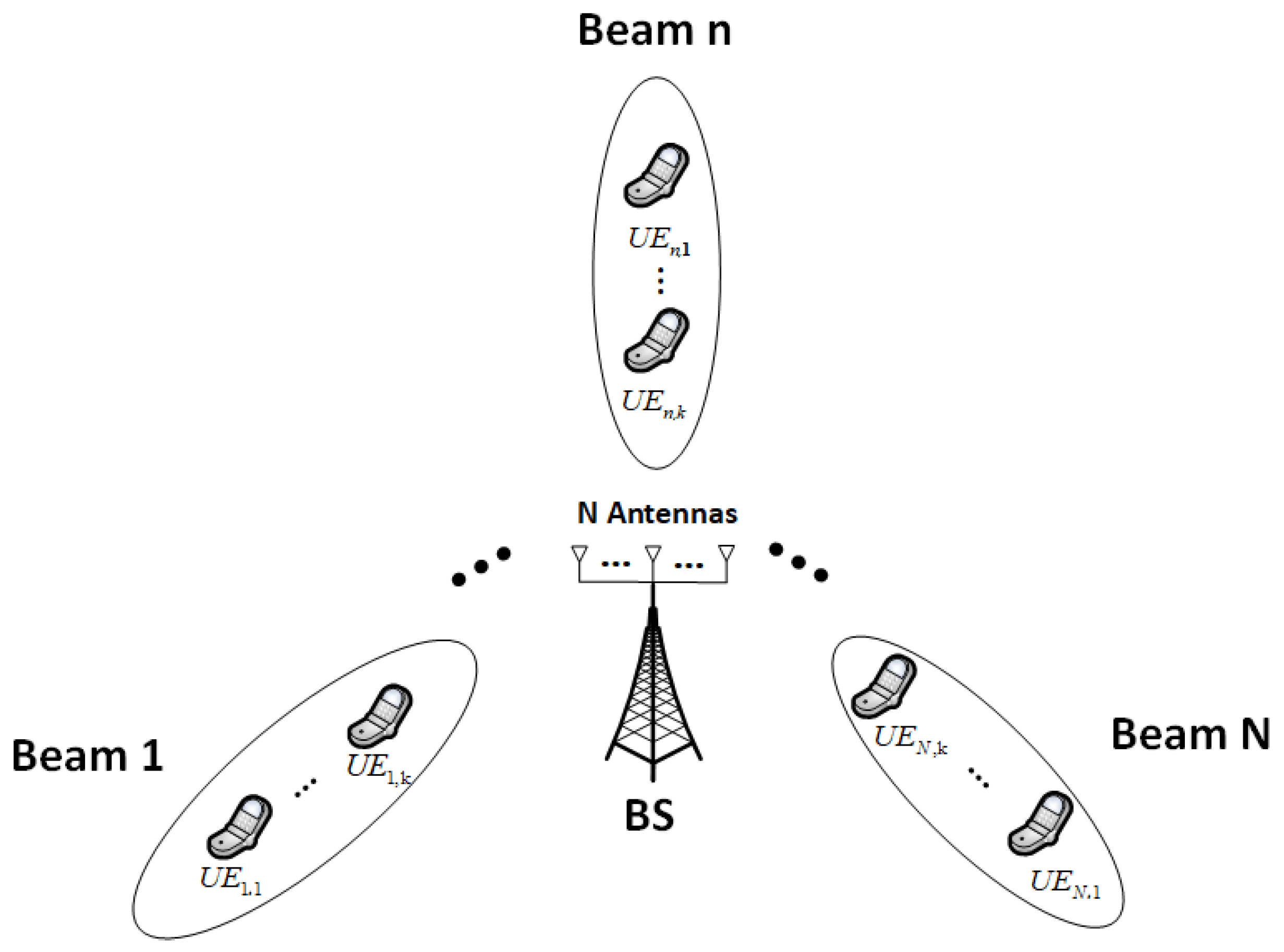
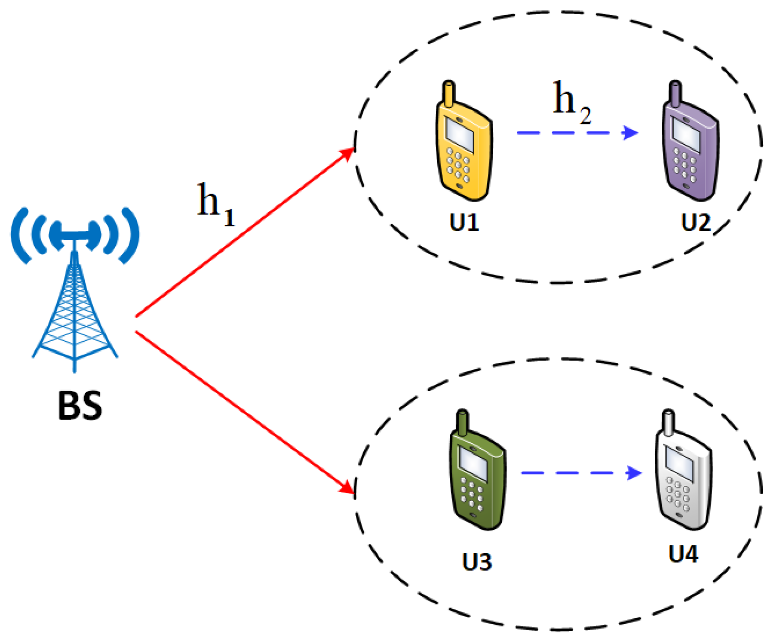
2. System Model

As technology evolves, so do wireless systems, and NOMA technology is gaining interest in 6G due to its advantages in improving overall frequency efficiency, first by superimposing users in the time and frequency domains and then using SIC to achieve the main points in the multiple access channel.

Due to SIC error propagation, the number of customers permitted for PD-NOMA is quite limited. Discussed with NOMA in mind, the meaning of equity is inconsistent on the topic of distribution. Due to the uncertainty of the specific locations of the different users, a rational way of allocating power on account of random geometry is proposed and cited. In practice, the number of cells is so large that locating users to specific cells while increasing the total rate of the system will become very difficult, although most articles address NOMA. The authors of [16] used related theoretical techniques to solve the challenge of increasing the total rate in a multi-cell system while localizing the users. The situation may be improved by considering various sorts of service needs in various cells, and [17] proposes a power allocation method that takes various forms of data traffic into account. A network with excellent performance should have the ability to switch to OMA at any time since the advantages of PD-NOMA versus OMA depend to a large extent on the gain variation of the different channels. In order to allow the system to choose amongst them, the authors of [18] recently proposed a utility charge that accounts for the expenses and advantages associated with each MAC mode. The NOMA technique is widely used for multiplexed communication between terminals and two receiver units [19,20], i.e., device-to-device (D2D) communication, where many users in the system are greatly amplified when PD-NOMA is combined with orthogonal frequency division multiplexing (OFDM). Various solutions such as greedy algorithms were then proposed in order to solve the user and power problems. Figure 1 depicts a MIMO-NOMA communication configuration for groups of users. Since NOMA is used for transmission, SIC detection is employed on the user side.

Figure 2 shows the downlink SWIPT-assisted cooperative NOMA system structure. If U1 and U2 are on the same frequency band, the BS can serve both at the same time. There is no direct transmission route from BS to U2 due to physical obstacles or excessive shading during transmission. The introduction of the cooperative relay U1 solves this problem, and U1 will help the BS to overcome the physical obstacles and realize the information transmission from U2 to the BS. Because U1 has a limited amount of energy, it first gathers energy from the BS signal before relaying it. $h_1$ and $h_2$ denote the channels from U1 to BS and from U2 to BS. Rayleigh fading is experienced by all channels, i.e., $h_i\sim \mathcal{C}\mathcal{N}\left(0,{\lambda }_i\right), i\in \left\{1,2\right\}$.

Similarly, a constant-linear-constant (CLC) EH model is considered. Accordingly, U1 terminal energy is described as:

$$E=\{\begin{array}{cc}0,& \xi \in \left[0,P^{sen}\right],\\ \eta \left(\xi -P^{sen}\right)t,& \xi \in \left[P^{sen},P^{sat}\right],\\ \eta \left(P^{sat}-P^{sen}\right)t,& \xi \in \left[P^{sat},+\infty \right),\end{array}$$

(1)

The received power at U1 is $\xi$, The sensitivity power threshold for EH is $P^{sen}$, the saturation power threshold for EH is $P^{sat}$, $t$ is the duration of the EH, and $\eta (0<\eta <1)$ is the energy efficiency.

3. Methods

We first describe the downlink transmission protocol and then analyze the user rate for the downlink transmission protocol.

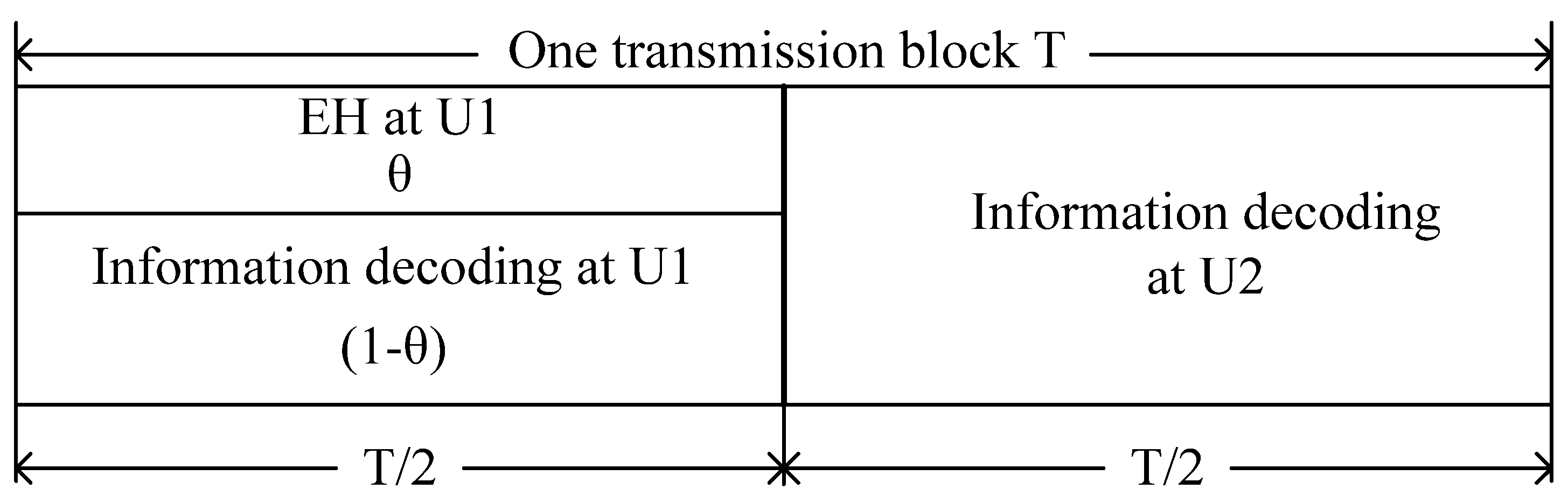
3.1. Transmission Protocol

The cooperative NOMA transmission protocol supported by the downlink SWIPT is shown in Figure 3. The downlink transmission period is T, equally divided into two phases before and after T/2. The BS sends a signal in the first phase, which overlaps the information of the two users. At the same time, U1 receives a certain amount of signal from the BS and uses it in two ways, half for EH and the other half for decoding the information. Then, provided that U1 has successfully decoded the overlapping message, U1 will have enough energy to send U2′s signal, and U2 gets the forwarded signal to decode its own message. Otherwise, U1′s message will fail.

3.2. Achievable Rates

The BS transmits a superimposed signal in the first phase,

$$x=W_1{x}_1+W_2{x}_2,$$

(2)

where $x_1$ and $x_2$ are the signals, $W_1$ and $W_2$ are the precoding vectors.

Then the expression for U1 is:

$$y_1=H_1{W}_1{x}_1+H_1{W}_2{x}_2,$$

(3)

where $H_1$ denotes the channel vector of BS-U1.

According to the power splitting scheme [18], U1 splits $\sqrt{\theta }{y}_1\left(t\right)$ ($0\le \theta \le 1$) for EH, where $\theta$ is the power-splitting ratio. In particular, since the correlation analysis has been carried out on the CLC EH model in (1), the expression at U1 is

$$E=\{\begin{array}{cc}0,& \theta p|H_1{|}^2\in \left[0,P^{sen}\right],\\ \eta (\theta p|H_1{|}^2-P^{sen})\frac{T}{2},& \theta p|H_1{|}^2\in \left[P^{sen},P^{sat}\right],\\ \eta \left(P^{sat}-P^{sen}\right)\frac{T}{2},& \theta p|H_1{|}^2\in \left[P^{sat},+\infty \right).\end{array}$$

(4)

Meanwhile, upon remaining fraction $\sqrt{1-\theta }{y}_1\left(t\right)$, U1 first detects $x_2$ and then detects $x_1$ by SIC, with signal to interference and noise ratio (SINRs)

$${\gamma }_{12}=\frac{{\left|H_1{W}_2\right|}^2}{{\left|H_1{w}_1\right|}^2+{\sigma }^2},$$

(5)

and

$${\gamma }_{11}=\frac{{\left|H_1{W}_1\right|}^2}{{\sigma }^2},$$

(6)

respectively, where the additive Gaussian white noise is when U1 detects $x_1$ and $x_2$. U1 forwards $x_2$ to U2 by All collected energy over the T/2 block. Accordingly, the transmit power of U1 can be expressed as:

$$p_1=\frac{E}{T/2}=\{\begin{array}{cc}0,& \theta p|H_1{|}^2\in \left[0,P^{sen}\right],\\ \eta (\theta p|H_1{|}^2-P^{sen}),& \theta p|H_1{|}^2\in \left[P^{sen},P^{sat}\right],\\ \eta \left(P^{sat}-P^{sen}\right),& \theta p|H_1{|}^2\in \left[P^{sat},+\infty \right).\end{array}$$

(7)

Upon the forwarded signal from U1, U2 detects $x_2$ with SNR

$${\gamma }_{22}=\frac{p_1|h_2{|}^2}{{\sigma }^2}$$

(8)

where $h_2$ denotes the channel vector of U1-U2. Obviously, the achievable rates are

$$R_{11}=\frac{1}{2}{\mathit{log}}_2(1+{\gamma }_{11})$$

(9)

and

$$R_{12}=\frac{1}{2}{\mathit{log}}_2(1+{\gamma }_{12}),$$

(10)

respectively.

The rate of $x_2$ is

$$R_{22}=\frac{1}{2}{\mathit{log}}_2(1+{\gamma }_{22})$$

(11)

4. DRL-Based User-Pairing NOMA Scheme

The authors developed a methodology for getting the best power allocation factors using the deep reinforcement learning (DRL) scheme in their paper. This research also uses the user pairing approach to determine the best power allocation. The DRL environment is then used to transform the user pairing scheme. The Deep Q-learning network (DQN) technique is used to study average sum rate performance as well as optimal power allocation. Finally, the algorithm with the description of the entire procedure is presented.

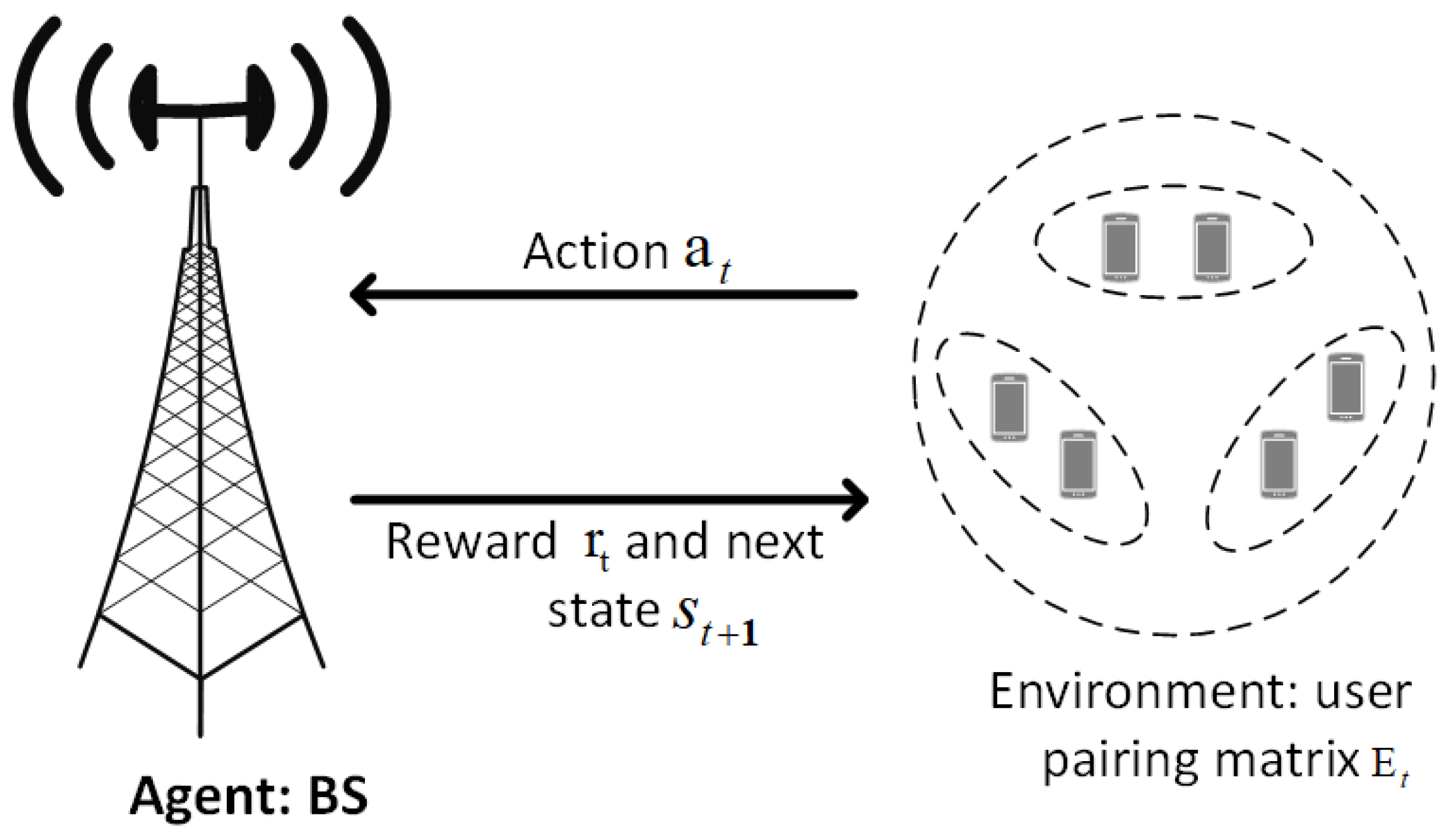
4.1. DRL Based Downlink SWIPT

In this sub-section, the user-pairing NOMA framework is transformed to the DRL environment. The DRL scenario is demonstrated in Figure 4. Agent, state and environment, action, target and reward, and policy are the main components of the DRL algorithm, expressed below: In a real-time propagation context, RL seeks to train an agent how to do a job. The agent is a policy maker as well as a learner. The agent responds by sending actions to the environment after receiving observations and a reward from the environment. The agent incorporates both a policy and a learning algorithm. BS serves as an agent in DRL. The “state” of the DRL technique is defined as the change that results from each interaction between the “agent” and external elements (acting as an “object”). Given the DRL situation and the recommended problem of adaptability for different users of NOMA, the DRL environment can currently only represent the user pairing matrix $E_t$. The agent may only do one “activity” every step while interacting with the environment, and each component in $G_1$ is a $2\times 2$ line matrix and each component in $G_2$ is a column. The NOMA system marks a period of time as a training period during each of which the agent interacts with the environment, changing the state from the present one to the next one. The agent must choose an appropriate action based on unique strategies in the current state $s_t$ since the various actions have different environmental implications. The action space of $A_t$ may be described by the NOMA system as $A_t=\left\{u_t^{N+1},u_t^{N+2},\dots \dots ,u_t^N\right\}$, with the action $t$ representing $u_t^p\left(p\in \left\{N+1,N+2,\dots .,N\right\}\right)$ at step $t$. Because wireless users have an influence on the row representation $G_1$ of the user pairing matrix, Let us say that a transfer partner is created when user $t$ selects user $p$, which is interpreted as up $u_t^p=1$, in every step $t$; otherwise, $u_t^p=0$. A positive or negative payment is received after the agent has completed the work. The agent’s objective is to discover and recognize a policy that will maximize the cumulative discount payment, which is determined at each training session by multiplying the present instant benefit by a discount factor. In our NOMA system, the immediate reward may be calculated as $r_t=r_t^{\pi }\left(s_t,a_t\right)$, where $s_t$ represents the state and $a$ represents the action taken in step $t$. The average sum rate of the $t^{\mathrm{th}}$ user is $r_t$, whereas the sum rate of users who are moved on the same user pair is $r_t$. If a user pair contains many users, the system will set the current payment to 0, which is the goal of the DQN algorithm, which is to maximize the discount. The process is selected by the agent in the same way that the policy is selected by the agent. The DQN approach uses the $\epsilon$-Greedy policy to select an action. The probability of occurrence of the highest state value $Q\left(s_t,a_t\right)$ of this action is $1-\epsilon$, which is to randomly select an action with probability $\epsilon$. To prevent the selected algorithm from being tuned locally to the optimal solution, the agent can use processes to investigate unknown actions and conditions.

4.2. Optimal Power Allocation and User Pairing Based on Q-Learning Algorithm

The average sum-rate of D/L NOMA UEs is the “reward”, which represents the reward at time $t$, expressed below,

$$R={{\displaystyle \sum }}_{n=1}^N{{\displaystyle \sum }}_{k=1}^K{\log }_2\left(1+\frac{{\alpha }_{n,k}{p}_n{\left|{\widehat{z}}_{n,k}\left(\tau \right)w_n\right|}^2}{I_{n,k}^U+{\sigma }_n^2}\right)$$

(12)

The sum-rate computed using ${\hat{z}}_{n,k}\left(\tau \right)$ is represented as $R$. In $\mathrm{Q}$-learning, the Q-function updates $R$ on a regular basis, whereas $R$ calculates ${\hat{z}}_{n,k}\left(\tau \right)$. The user pairing index and the power allocation factors are both determined simultaneously using $Q$-learning. Furthermore, given system state $s$ and action $a,Q\left(s^t,{\theta }^t\right)$ denotes the BS’s Q-function,

$$Q\left(s^t,{\theta }^t\right)\leftarrow \left(1-\beta \right)Q\left(s^t,{\theta }^t\right)+\beta \left[R\left(s^t,{\theta }^t\right)+\delta \underset{{\theta }^{\prime }}{\max }Q\left(s^{t+1},{\theta }^t\right)\right]$$

(13)

where $\beta \in \left(0,1\right]$ denotes the importance of recent learning experiences. The discount factor $\delta \in \left[0,1\right]$ determines the importance of present and future benefits. The complete dynamic user pairing and power distribution methodology for the NOMA system with DRL is shown in the diagram below Algorithm 1:

Algorithm 1 The proposed NOMA system with the DRL

Input: iterations $T$, action set $A$, decay factor $\gamma$, Actor neural network $\pi (a|s,\theta )$, Critic neural network $v\left(s,w\right)$

Output: Actor network parameters $\theta$, Critic network parameters $w$

Initialize $\theta \leftarrow {\theta }_0$, $w\leftarrow w_0$

for $t$ from 1 to $T$($S$ is not terminal):

$A\sim \pi (·|S,\theta )$, take action $A$, observe $S^{\prime }$ $R$

Collect and save sample $\left\{S,A,R,S^{\prime }\right\}$

Calculate TD-error $\delta =R+\gamma v\left(S^{\prime },w\right)-v\left(S,w\right)$ through Citric network

Update Critic network $w$ according to Mean square error loss function ${\displaystyle \sum }{\left(R+\gamma v\left(S^{\prime },w\right)-v\left(S,w\right)\right)}^2$

Update Actor network $\theta =\theta +\alpha {\nabla }_{\theta }\log \pi (A|S,\theta )\delta$

end for

return $\left(\theta ,w\right)$

5. Simulation Results

5.1. Simulation Settings

This section shows the simulation results to justify the end-to-end performance of DRL based NOMA by adopting the DQN algorithm as a typical DRL implementation. We also simulate the end-to-end system performance of the other three approaches, namely simple deep neural network (DNN) NOMA, SC-NOMA, and conventional TDMA scheme considering the optimal power allocation to make a comparison.

The BS specifications are 512 physical antenna elements (16, 16, 2, 256 elements each polarization) in a cross-pol array. Physical antenna components: 90-degree beamwidth, half-wavelength spacing between rows and columns, and 5 dBi maximum gain per physical element. If the polarizations are not coherently mixed, the maximum EIRP are 54 dBm and 60 dBm, respectively, with a noise figure of 5 dB. The following are the UE settings: Dual panel cross-pol array with best-panel selection at UE, with two panels orientated back-to-back. Each panel consists of 32 physical parts, with 16 parts per polarization, and the TX power transmitted to the active panel element is 23 dBm. A physical antenna array panel has elements with a 90-degree beamwidth, half-wavelength spacing between rows and columns, and a maximum gain of 5 dBi per physical element. In all circumstances, the maximum EIRP is 40 dBm (provided all antenna components can be coherently integrated), with a noise figure of 9 dB. The simulation parameters are shown in

Table 1. Basic simulation parameters.

Parameter	Numerical Value
Distance between two users	12 m
Net transfer bandwidth	800 MHz
Carrier frequency	100 GHz
Transmit power of BS	40–100 W
Path loss index of the channel	3
AWGN noise spectral density	−170 dBm/Hz
Quality of service threshold	2.5 bps/Hz
Noise figure	5 dB

. It has been assumed that the BS is situated at the center, with the UEs dispersed randomly about the cell at distances ranging from 50 to 250 m. With respect to machine learning simulation, we adopt an open-source tool developed from the Google library TensorFlow running on Python.

In deep learning, we usually use floating point operations per second (FLOPS) to measure the complexity of the neural network model. The Actor-Critic model consists of two parts, one is the policy function generated by Q network, and the other is to evaluate the quality of Q network output policies. After updating Q network continuously through a large number of episodes, the Q network can give reasonable action A for each state S. Therefore, in the real calculation FLOPS aspect of the Actor-Critic model, we only need to calculate the Q network to meet the requirements of the real environment. The choice of FLOPS for different network models Figure 1 of ref [21] and the computing power of different devices is a trade-off issue [22]. We will choose a reasonable Q network model between accuracy and devices computing speed.

5.2. Simulation Analysis by Considering Frequency Flat Fading Conditions without Node Mobility

In the analysis, the simulation results in different parameter settings are shown in

Table 2. Simulation results in different parameter settings.

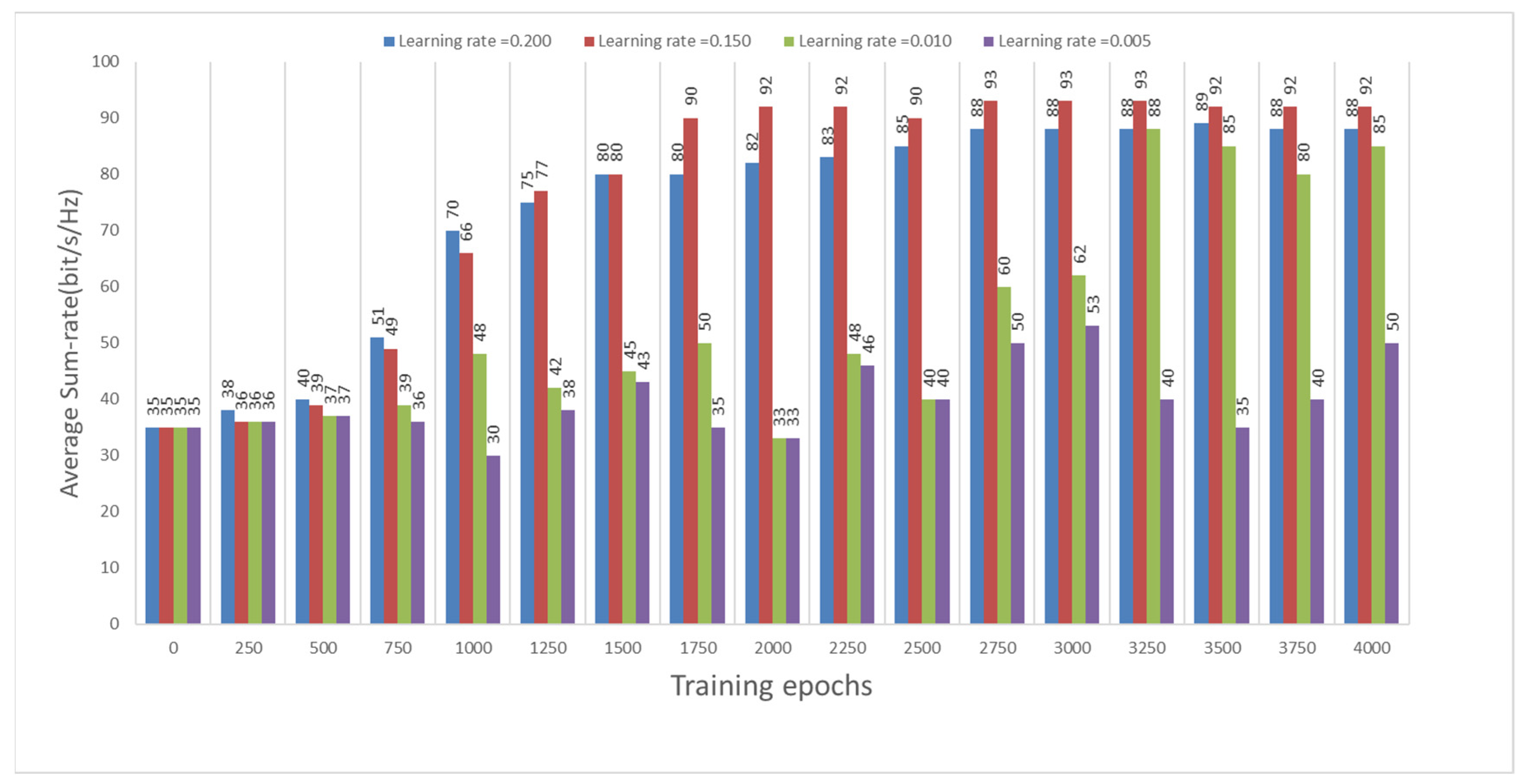
Parameter		Minimum Epochs of Achieving Convergence (k)	Average Sum-Rate (bit/s/Hz)
learning rate lr	lr = 0.005	2.7	53
	lr = 0.010	3.2	80
	lr = 0.150	2.0	93
	lr = 0.20	2.7	88
decay factor $\gamma$	$\gamma =0.99$	3.0	80
	$\gamma =0.95$	2.5	90
	$\gamma =0.90$	3.2	82
exploration rate $ϵ$	$ϵ=0.10$	2.0	93
	$ϵ=0.15$	2.8	88

. The average sum rate is represented as the “average cumulative reward,” and the BS acts as an “agent.” Figure 5 demonstrates the learning graphs; this shows the average sum rate over the entire course of BS. In the simulation, we consider 30 UEs. The best end-to-end system performance can be achieved with a learning rate of 0.1500, after 3900 epochs, as the average sum rate or cumulative reward converges to around 100 Mbps. The DQN scheme, in addition, converges faster when the learning rate is 0.2000, but does not attain the maximum throughput (or average sum rate). This problem may be explained that when the learning rate is high and the gradient update speed is too quick, causing the optimal solution to slide. Meanwhile, the DQN algorithm fails to converge when the learning rate is set to 0.010 or 0.005. This is because when the learning rate is low, gradient updating is likewise sluggish. As a result, the training process will not be able to converge in less than 4000 epochs.

The DQN system has surpassed the DNN, conventional TDMA, and SC-NOMA schemes, as can be seen in Figure 6. Furthermore, it is simple to show that TDMA performance is superior than SC-NOMA performance. It turns out that expanding the number of customers on the same subcarrier without paying for it is not feasible. The learning rate in simulation is set as 0.20. The DQN NOMA algorithm surpasses the DNN NOMA scheme, proving that a substantially higher data rate than the Nyquist Shannon rate can achieve. The DQN NOMA algorithm employs the DL approach to calculate the Q value. It is clear that the DQN NOMA method can use DL symbol training to extract information. Furthermore, the storage and retrieval of Q values are made more difficult by the abundance of data symbols. As a result, in terms of overall conversion efficiency and SE, better than the DNN NOMA method is the DQN NOMA algorithm. Furthermore, the DQN-NOMA approach outperforms TDMA and random user pairing. This is true since the evaluated NOMA system’s ideal transmission pairing employs 8 UEs. Because only one UE is relayed on a subchannel, the methodology requires more spectrum than the TDMA strategy. By using capabilities in both the frequency and output domains, the NOMA strategy may greatly increase data transmission rates.

6. Conclusions

This paper has developed a 6G downlink MIMO-NOMA system that supports simultaneous wireless information and power transfer. In order to improve overall performance, we apply DRL to optimize user pairing and radio resource allocation. The performance of our designed MIMO-NOMA system is validated by simulation results. With the appropriate fitting of the neural network, the DRL method can determine the ideal pairing and power distribution for each user with satisfying convergence speed.

References

- Wang, C.-X.; Huang, J.; Wang, H.; Gao, X.; You, X.; Hao, Y. 6G Wireless Channel Measurements and Models: Trends and Challenges. IEEE Veh. Technol. Mag. 2020, 15, 22–32. [Google Scholar] [CrossRef]
- de Lima, C.; Belot, D.; Berkvens, R.; Bourdoux, A.; Dardari, D.; Guillaud, M.; Isomursu, M.; Simona Lohan, E.; Miao, Y.; Barreto, A.N.; et al. Convergent Communication, Sensing and Localization in 6G Systems: An Overview of Technologies, Opportunities and Challenges. IEEE Access 2021, 9, 26902–26925. [Google Scholar] [CrossRef]
- Tataria, H.; Shafi, M.; Molisch, A.F.; Dohler, M.; Sjöland, H.; Tufvesson, F. 6G Wireless Systems: Vision, Requirements, Challenges, Insights, and Opportunities. Proc. IEEE 2021, 109, 1166–1199. [Google Scholar] [CrossRef]
- Rezvani, S.; Jorswieck, E.A.; Joda, R.; Yanikomeroglu, H. Optimal Power Allocation in Downlink Multicarrier NOMA Systems: Theory and Fast Algorithms. IEEE J. Sel. Areas Commun. 2022, 40, 1162–1189. [Google Scholar] [CrossRef]
- Mothukuri, V.; Khare, P.; Parizi, R.M.; Pouriyeh, S.; Dehghantanha, A.; Srivastava, G. Federated-Learning-Based Anomaly Detection for IoT Security Attacks. IEEE Internet Things J. 2022, 9, 2545–2554. [Google Scholar] [CrossRef]
- Hui, H.; Zhou, C.; Xu, S.; Lin, F. A novel secure data transmission scheme in industrial internet of things. China Commun. 2020, 17, 73–88. [Google Scholar] [CrossRef]
- Tseng, L.; Wong, L.; Otoum, S.; Aloqaily, M.; Othman, J.B. Blockchain for Managing Heterogeneous Internet of Things: A Perspective Architecture. IEEE Netw. 2020, 34, 16–23. [Google Scholar] [CrossRef]
- Qiu, C.; Yao, H.; Jiang, C.; Guo, S.; Xu, F. Cloud Computing Assisted Blockchain-Enabled Internet of Thing. IEEE Trans. Cloud Comput. 2022, 10, 247–257. [Google Scholar] [CrossRef]
- Xiang, Z.; Yang, W.; Cai, Y.; Ding, Z.; Song, Y.; Zou, Y. NOMA-Assisted Secure Short-Packet Communications in IoT. IEEE Wirel. Commun. 2020, 27, 8–15. [Google Scholar] [CrossRef]
- Dai, L.; Wang, B.; Yuan, Y.; Han, S.; Chih-lin, I.; Wang, Z. Non-orthogonal multiple access for 5G: Solutions, challenges, opportunities, and future research trends. IEEE Commun. Mag. 2015, 53, 74–81. [Google Scholar] [CrossRef]
- Suo, L.; Li, H.; Zhang, S.; Li, J. Successive interference cancellation and alignment in K-user MIMO interference channels with partial unidirectional strong interference. China Commun. 2022, 19, 118–130. [Google Scholar] [CrossRef]
- Liu, X.; Zhang, X. NOMA-Based Resource Allocation for Cluster-Based Cognitive Industrial Internet of Things. IEEE Trans. Ind. Inform. 2020, 16, 5379–5388. [Google Scholar] [CrossRef]
- Nezhadmohammad, P.; Abedi, M.; Emadi, M.J.; Wichman, R. SWIPT-Enabled Multiple Access Channel: Effects of Decoding Cost and Non-Linear EH Model. IEEE Trans. Commun. 2022, 70, 306–316. [Google Scholar] [CrossRef]
- Luo, Y.; Pu, L. Practical Issues of RF Energy Harvest and Data Transmission in Renewable Radio Energy Powered IoT. IEEE Trans. Sustain. Comput. 2021, 6, 667–678. [Google Scholar] [CrossRef]
- Ding, Z. Harvesting Devices’ Heterogeneous Energy Profiles and QoS Requirements in IoT: WPT-NOMA vs BAC-NOMA. IEEE Trans. Commun. 2021, 69, 2837–2850. [Google Scholar] [CrossRef]
- Baidas, M.W.; Bahbahani, Z.; Alsusa, E. User association and channel assignment in downlink multi-cell NOMA networks: A matching-theoretic approach. EURASIP J. Wirel. Commun. Netw. 2019, 2019, 220. [Google Scholar] [CrossRef] [Green Version]
- Mokhtari, F.; Mili, M.R.; Eslami, F.; Ashtiani, F.; Makki, B.; Mirmohseni, M.; Nasiri-Kenari, M.; Svensson, T. Download elastic traffic rate optimization via NOMA protocols. IEEE Trans. Veh. Technol. 2019, 68, 713–727. [Google Scholar] [CrossRef]
- Baghani, M.; Parsaeefard, S.; Derakhshani, M.; Saad, W. Dynamic non-orthogonal multiple access (NOMA) and orthogonal multiple access (OMA) in 5G wireless networks. IEEE Trans. Commun. 2019, 69, 1. [Google Scholar]
- Ghous, M.; Hassan, A.K.; Abbas, Z.H.; Abbas, G. Modeling and analysis of self-interference impaired two-user cooperative MIMO-NOMA system. Phys. Commun. 2021, 48, 101441. [Google Scholar] [CrossRef]
- Ghous, M.; Abbas, Z.; Hassan, A.; Abbas, G.; Baker, T.; Al-Jumeily, D. Performance Analysis and Beamforming Design of a Secure Cooperative MISO-NOMA Network. Sensors 2021, 12, 4180. [Google Scholar] [CrossRef]
- Tan, M.; Le, Q. Efficientnet: Rethinking model scaling for convolutional neural networks. In Proceedings of the International conference on machine learning, PMLR 2019, Long Beach, CA, USA, 9–15 June 2019; pp. 6105–6114. [Google Scholar]
- Huang, S.Y.; Chu, W.T. Searching by generating: Flexible and efficient one-shot NAS with architecture generator. In Proceedings of the IEEE/CVF Conference on Computer Vision and Pattern Recognition, Nashville, TN, USA, 20–25 June 2021; pp. 983–992. [Google Scholar]