Modeling and Simulation of Magnetic Balance Current Sensor Based on Magnetic Scalar Potential Volume Integral

Abstract

In this paper, a field–circuit combined simulation method, based on the magnetic scalar potential volume integral equation (MSP-VIE) and its fast algorithms, are proposed for the transient simulation and nonlinear distortion analysis of the magnetic balance current sensor. The magnetic part of the sensor is modeled and simulated by MSP-VIE with the field matrices extracted by the method of moments. By directly implementing the magnetic field equation in the circuit, these field matrices can be regarded as equivalent circuit parameters of the magnetic part, to construct the corresponding SPICE model. Finally, the field–circuit combined model of the entire sensor is unified in a circuit, so with the SPICE solver, the transient simulation is accomplished in the time domain. Moreover, aiming at the time-consuming problem, this paper presents a corresponding fast method to accelerate the simulation. The comparison of measurement and simulation demonstrates that the proposed method not only realizes the transient simulation of the whole sensor, but also simulates some hidden performance details; thus, it can be applied to practical engineering, to guide and test the early design of the product.

1. Introduction

Magnetic balance currents have the advantages of wide measurement range, fast response speed, high measurement accuracy, good linearity, and operating frequency bandwidth [1]. In recent years, the research has focused on system-on-chip [2], thermal drift [3], magnetic core structure [4] etc. In different application environments, sensors needs to be designed with different performance, accordingly. Moreover, due to the complexity of the application environment, the sensor will have some faults when it is disturbed by the outside world, so it is necessary to analyze the cause of the breakdown. However, it is difficult to test a circuit in the actual working conditions. Thus, modelling and simulation is of great significance for design and improvement. In many situations, such as checking the hidden danger, testing conjecture etc., it is very convenient to have a model.

The sensor is composed of the magnetic part (magnetic core, coil) and the circuit part (Hall element, circuit board), so the overall performance is closely related to the two parts [4]. Because of the closed-loop working principle, the magnetic part and the circuit part must be considered comprehensively and simulated jointly. Consideration should not only be given to: the shape of the magnetic core; the magnetic properties of the magnetic core material; the winding mode of the coil; and the positional relationship between the coil and the magnetic core; but also the output characteristics of the magnetic part, which should match the circuit part.

Ultimately, the sensor needs closed-loop simulation and field–circuit combined simulation. Aiming at this problem, it is necessary to establish an equivalent circuit model, considering various factors of magnetic core. Some analysis methods and solutions have been proposed in relevant papers. Pankau J [5] regarded the magnetic parts of the sensor as a single-phase transformer, and then adopted the equivalent circuit model to realize the high-frequency modeling and accomplish the field–circuit combined simulation. Pejovic P [6] and Ai X [7] took the sensor as a current transformer and established the equivalent circuit model through the transformation function, and accordingly conducted transient analysis on the low-frequency characteristics and sensitivity.

Additionally, Sixdenier utilized finite element simulation to obtain magnetic field parameters, such as magnetic flux, and magnetic flux leakage of the magnetic core, and constructing the magnetic equivalent circuit, based on these module units, ultimately implemented the magnetic circuit modeling and field–circuit combined analysis [8]. To a certain degree, these methods can be used to implement the overall analysis of the sensor, but in fact, they have some drawbacks. These models are simplified a lot and it is difficult to consider the core structure, coil position and other factors in a simple equivalent model. Moreover, some papers have reported sensor simulation and optimization methods using finite element software [9,10]. The circuit element model in the finite element analysis is not accurate, and due to many grids in the air, the closed circuit analysis of magnetic circuit and electric circuit is difficult to converge.

There are some more accurate magnetic equivalent circuit models outside the field of magnetic balance sensors, such as magnetic shielding effectiveness in Rogowski coils [11], transformers [12,13], and switched reluctance motors [14]. However, due to the differences in structure and working-principle circumstances, these models can only be used in their respective fields.

Different from the above traditional methods, [15] reported a transient analysis method based on magnetic field integral equation, to research the fluxgate sensor. The main idea in the paper is to use magnetic scalar potential volume integral equation (MSP-VIE) to extract the magnetic field equation and matrix data, which serve as the equivalent circuit parameters, to construct the corresponding SPICE model, and finally utilize the SPICE solver to realize the field–circuit combined simulation.

This paper further improves and realizes the matrix parameter extraction and the circuit modeling based on MSP-VIE, and applies it to a closed-loop simulation of a magnetic balance current sensor. In addition, this paper also develops a fast method of solving the time-consuming problem in the SPICE simulation. The simulation and measurement results show that this method can not only implement closed-loop simulation and field–circuit combined simulation, but also simulate some hidden performance details, by accurately considering the magnetic core. This method can be applied to practical engineering, in order to guide, optimize and test the product design.

2. Theory and Equation

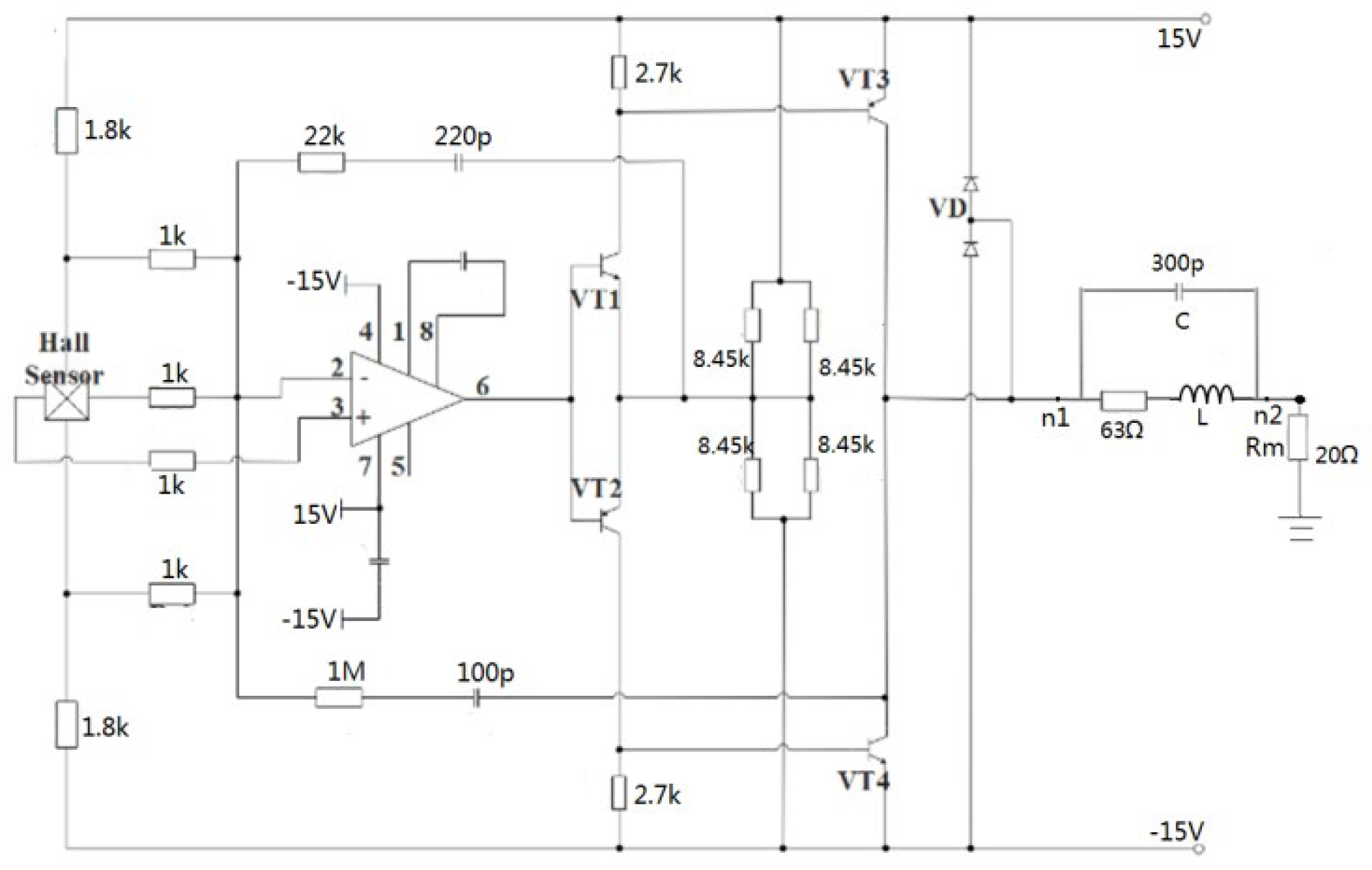
2.1. Working Principle of Magnetic Balance Current Sensor

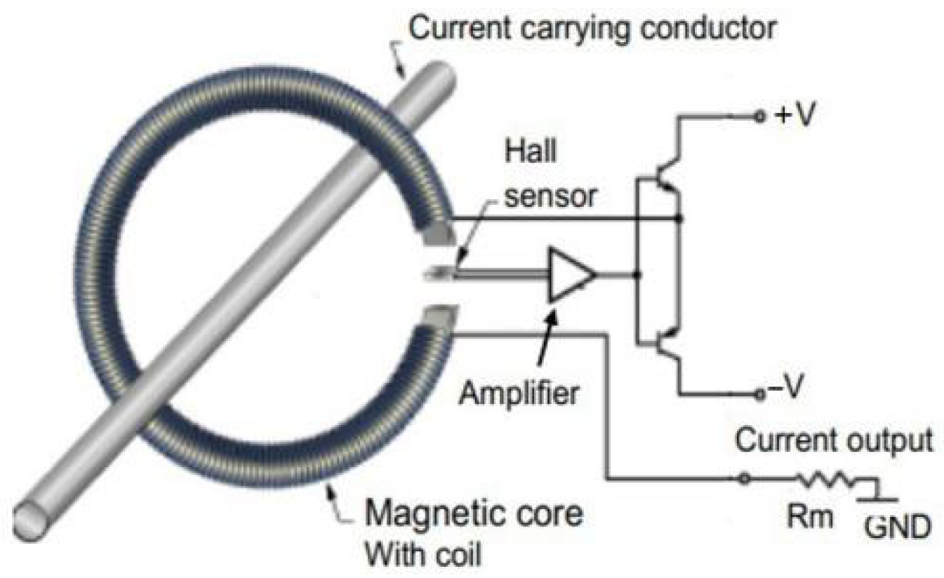
As shown in Figure 1, the measured current is loaded on the straight wire and passes through the magnetic core. The sensor is composed of a magnetic core, circuit, Hall generator and compensation coil on the core. The Hall element, placed in the air gap of the magnetic core, detects the magnetic induction intensity and drive; the electric circuit then supplies a secondary current (Is) to the coil, which creates a flux equal in amplitude, but opposite in direction, to the flux created by the primary current.

The secondary winding acts as a current transformer at higher frequencies. At low frequencies, the sensor operates using the Hall generator. At higher frequencies the secondary coil operates as a current transformer, providing a secondary output current again, defined by the turns ratio and converted to a voltage by the measuring resistor.

To give an order of magnitude, the typical number of secondary turns is NS = 1000…5000 and the secondary current is usually between IS = 25…300 mA, although it could be as high as 2 A. The unique design of closed-loop transducers provides an excellent bandwidth.

2.2. Magnetic Scalar Potential Volume Integral Equation

To realize the field–circuit combined simulation for the entire sensor, the magnetic part (coil, magnetic core and straight wire) should be processed first. Considering the low-frequency working condition, this paper uses a static magnetic field as an approximation.

In the excitation of the magnetic field, generated by external constant current source, magnetic materials will be magnetized. The magnetization behavior law is quantitatively defined by:

$${\rm M}(r)=\chi (r,H)H(r)$$

(1)

where ${\rm M}(r)$ is the magnetization, $H(r)$ is the magnetic field at point of coordinates $r$, and $\chi (r,H)$ is the nonlinear magnetic susceptibility.

At any point in space, the total magnetic field $H(r)$ is a vector sum of the reduced magnetic field $H_{\mathrm{d}}(r)$ generated by the magnetic material and the magnetic field source $H_0(r)$ created by the external current:

$$H(r)=H_0(r)+H_{\mathrm{d}}(r)$$

(2)

In the source-free region, the magnetic field is irrotational, so Equation (2) can be expressed by magnetic scalar potential as below [16]:

$$\mathsf{\varphi }(r)+\frac{1}{4\pi }{\displaystyle {\int }_{V^{\prime }}\chi (r^{\prime },H)\frac{\nabla \mathsf{\varphi }(r^{\prime })·(r-r^{\prime })}{{\left|r-r^{\prime }\right|}^3}}d{V}^{\prime }={\mathsf{\varphi }}_0(r)$$

(3)

where ${\mathsf{\varphi }}_0(r)$ is the source potential of $H_0(r)$ and $\mathsf{\varphi }(r)$ is the total scalar potential of $H(r)$, satisfying $H_0(r)=-\nabla {\mathsf{\varphi }}_0(r)$, $H(r)=-\nabla \mathsf{\varphi }(r)$. The integral domain $V^{\prime }$ denotes the magnetic core.

2.3. Solution with Method of Moments

To solve Equation (3), the magnetic material region is discretized with a linear tetrahedron, and the total scalar potential $\mathsf{\varphi }(r)$ is approximated with first-order nodal shape function:

$$\varphi \approx {\displaystyle \sum _{j=1}^N{\varphi }_j{N}_j}$$

(4)

where ${\varphi }_j$ and $N_j$ denote the unknown and shape function associated to the j-th mesh node, respectively. N is the number of total nodes.

Then the collocation method at mesh nodes is used to match Equation (4), and, finally, it leads to the solution of a system of algebraic equations:

$$\left[I+A\right]\mathsf{\varphi }={\mathsf{\varphi }}_0$$

(5)

$$A_{ij}=\frac{1}{4\pi }{\displaystyle \sum _m{\displaystyle {\int }_{V_m^{\prime }}{\chi }_m({\mathbf{r}}^{\prime },\mathbf{H})\frac{\nabla N_j({\mathbf{r}}^{\prime })·({\mathbf{r}}_i-{\mathbf{r}}^{\prime })}{{\left|{\mathbf{r}}_i-{\mathbf{r}}^{\prime }\right|}^3}}d{V}_m^{\prime }}$$

(6)

where $I$ denotes the unit matrix and $A$ is the impedance matrix, with each element calculated by Formula (6). $A_{\mathrm{ij}}$ is the impact of mesh elements with j-th node on i-th node potential. ${\displaystyle {\int }_{V_m^{\prime }}d{V}_m^{\prime }}$ expresses the volume integral at the m-th mesh element and M is the number of total elements.

The excitation potential on the right side of the Equation (5) can be obtained through Biot-Savart’s law (7) and path integral (8):

$$H_0(r)=\frac{1}{4\pi }{\displaystyle {\int }_{V^{\prime }}\frac{\overrightarrow{J}(r^{\prime })\times (r-r^{\prime })}{{\left|r-r^{\prime }\right|}^3}d{V}^{\prime }}$$

(7)

$${\mathsf{\varphi }}_0(r)={\displaystyle \int H_0(r)·dr}$$

(8)

The magnetic source field $H_0(r)$ include ${\mathbf{H}}_a$ and ${\mathbf{H}}_s$, which are induced by the measured current and the compensation coil current, ${\mathsf{\varphi }}_0(\mathbf{r})$ can be expressed as follows:

$${\mathsf{\varphi }}_0(\mathbf{r})={\displaystyle {\int }_{}^{}d\mathbf{r}·({\mathbf{H}}_a(\mathbf{r})}+{\mathbf{H}}_s(\mathbf{r}))$$

(9)

Within the tetrahedron region, the gradient of first-order nodal shape function is constant, which means the impedance matrix $A$ can be separated into three parts:

$$A=-D·{\mathsf{\chi }}_m·G$$

(10)

where ${\mathsf{\chi }}_m$ is a diagonal matrix comprising the magnetic susceptibility in each mesh element, it is a nonlinear part. The matrix $D$ and $G$ are independent of the magnetic material, they are the invariable parts. The element of them is expressed by:

$${\mathbf{D}}_{im}=\frac{1}{4\pi }{\displaystyle {\int }_{V_m^{\prime }}\frac{{\mathbf{r}}_i-{\mathbf{r}}^{\prime }}{{\left|{\mathbf{r}}_i-{\mathbf{r}}^{\prime }\right|}^3}}d{V}_m^{\prime }$$

(11)

$${\mathbf{G}}_{mj}=-\nabla N_j,\hspace{1em}{r}_j\in V_m$$

(12)

Furthermore, after normalizing and decomposing the excitation potential, the matrix equation can be obtained as follows:

$$\left[I-D·{\mathsf{\chi }}_m·G\right]\mathsf{\varphi }={\mathsf{\varphi }}_0=C{I}_a+K{I}_s$$

(13)

where I_a represents the amplitude of the straight wire current, I_s represents the amplitude of the coil current, C and K are the corresponding excitation vectors, respectively. From (7)–(9), the elements of them are expressed by:

$$C_i={\displaystyle \int d\stackrel{\rightharpoonup }{r}}·\frac{1}{4\pi S_a}{\displaystyle \int \frac{{\stackrel{\rightharpoonup }{n}}_a({\stackrel{\rightharpoonup }{r}}^{\prime })\times ({\stackrel{\rightharpoonup }{r}}_i-{\stackrel{\rightharpoonup }{r}}^{\prime })}{{\left|{\stackrel{\rightharpoonup }{r}}_i-{\stackrel{\rightharpoonup }{r}}^{\prime }\right|}^3}d{V}^{\prime }}$$

(14)

$$K_i={\displaystyle \int d\stackrel{\rightharpoonup }{r}}·\frac{1}{4\pi S_s}{\displaystyle {\int }_{}\frac{{\stackrel{\rightharpoonup }{n}}_s({\stackrel{\rightharpoonup }{r}}^{\prime })\times ({\stackrel{\rightharpoonup }{r}}_i-{\stackrel{\rightharpoonup }{r}}^{\prime })}{{\left|{\stackrel{\rightharpoonup }{r}}_i-{\stackrel{\rightharpoonup }{r}}^{\prime }\right|}^3}d{V}^{\prime }}$$

(15)

where $V^{\prime }$ is the volume of current, ${\stackrel{\rightharpoonup }{n}}_a({\stackrel{\rightharpoonup }{r}}^{\prime })$ is the direction of the measured current, ${\stackrel{\rightharpoonup }{n}}_s({\stackrel{\rightharpoonup }{r}}^{\prime })$ is the direction of the coil current, $I_s/S_s$ is the compensation coil current density, $I_a/S_a$ is the measured current density. In this paper, the measured current under test is equivalent to the ideal line current and the compensation coil is equivalent to the volume current model.

The second part of (13) is the reduced potential, and at i-th node ${\mathsf{\varphi }}_{di}$ is:

$${\mathsf{\varphi }}_{di}={\displaystyle \sum _m{\mathbf{D}}_{im}·{\mathbf{M}}_m}$$

(16)

$${\mathbf{M}}_m={\chi }_m{\displaystyle \sum _j{\mathbf{G}}_{mj}·{\mathsf{\varphi }}_j}$$

(17)

In particular, the modified Born iteration method is utilized to solve the nonlinear equation. The iterative formula is:

$$\left[I-D·{\mathsf{\chi }}_m^{(k-1)}·G\right]{\mathsf{\varphi }}^{(k)}={\mathsf{\varphi }}_0$$

(18)

In the iterative process, the initial value of ${\mathsf{\chi }}_m^{(0)}$ and ${\mathsf{\varphi }}^{(0)}$ should be given at the same time. Depending on the magnetization curve of the magnetic core and the iterative equation, the next iteration value can be obtained immediately.

With computer programming, these parameter matrices of the magnetic part can be extracted by MSP-VIE.

3. Spice Modeling Based on MSP-VIE

MSP-VIE and method of moments construct the full-wave electromagnetic model of the magnetic part and extract the matrix. The parameter matrices D, G, C, K in (13) can be regarded as the equivalent circuit parameters, to establish the equivalent circuit model.

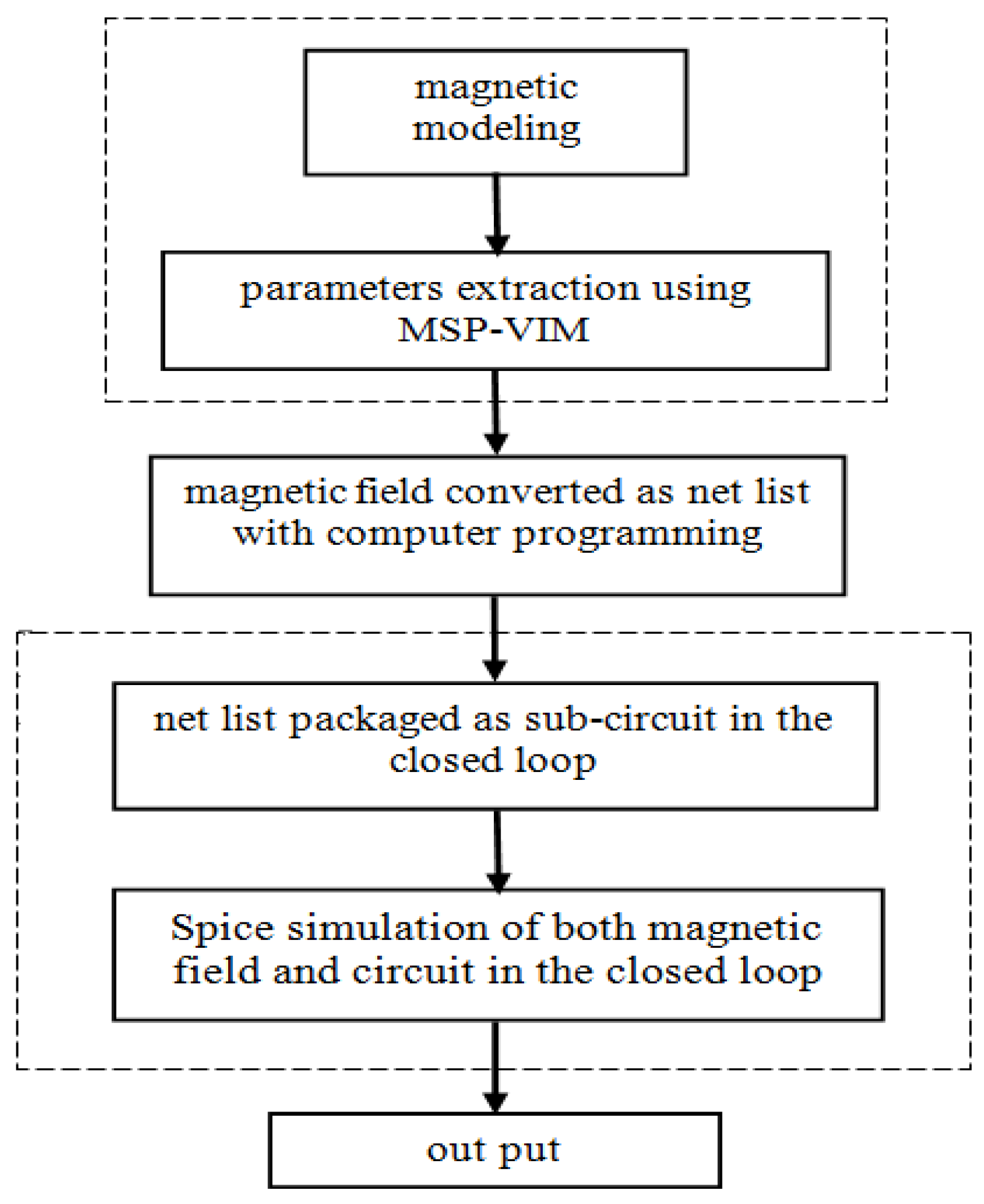
The flow chart of the modeling and simulation is shown in Figure 2. The parameter matrices D, G, C, K of the magnetic part can be extracted by MSP-VIE. Then the obtained parameters, as the equivalent circuit parameters of the magnetic component, are compiled to the netlist, as described in Section 3.3. Section 3.1 describes the equivalent relationship between the magnetic scalar potential equation and the Kirchhoff voltage equation corresponding to the netlist in Section 3.3. Section 3.2 describes the equivalent circuit of magnetic components considering parasitic parameters. With the netlist in Section 3.3, the magnetic field and circuit can be completed in the same platform: SPICE.

3.1. Circuit Realization of MSP-VIE

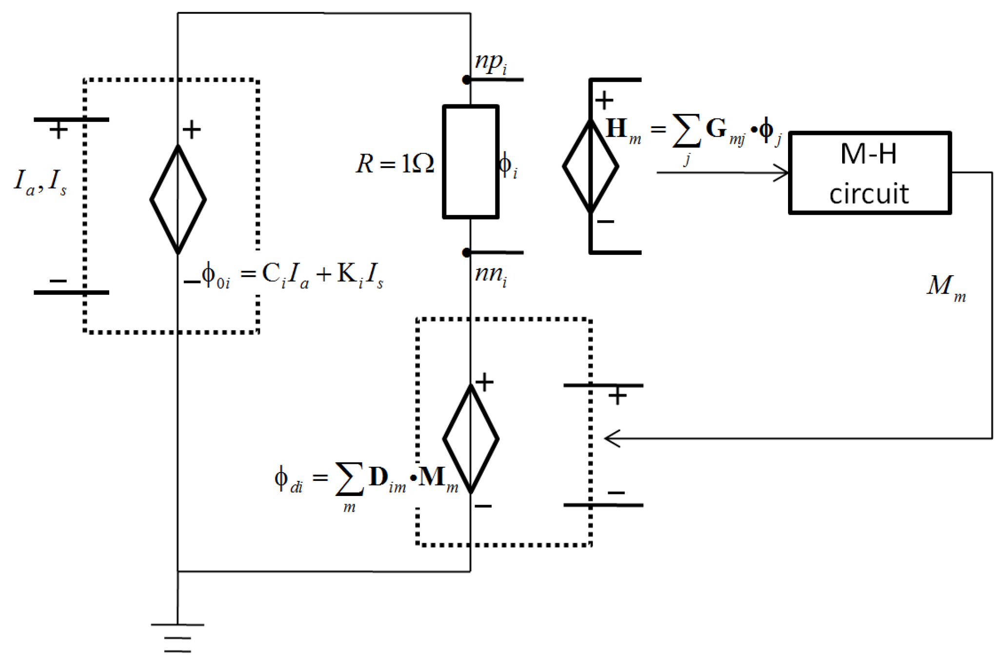
Once the geometry of the coil and core were known, the value of the coefficient matrices $D$, $G$, $C$, $K$ in (13) were determined and calculated by MSP-VIE. The magnetic scalar potential (Equation (13)) in the field was then equivalent to the Kirchhoff voltage equation in the circuit. Figure 3 shows the circuit implementation form of the i-th sub-equation in (13). The magnetic scalar potential in the field space can be treated as the node potential in the circuit. The voltage value across the resistor in Figure 3 is the total scalar potential at the i-th node. The voltage at node npi is the source potential at the i-th node ${\mathsf{\varphi }}_0(r)$, which is realized with a current-controlled voltage source. The voltage at node nni is the source potential at the i-th node ${\mathsf{\varphi }}_{\mathrm{d}}(r)$, which is realized with a voltage-controlled voltage source. The inputs are the measured current I_a and compensation coil current I_s. The compensation coil current I_s is obtained from the voltage node of the sampling resistor R_m in Figure 1. For convenience, the measured current I_a is also obtained from the voltage node.

Because the magnetic fields inside the magnetic core counteract each other in the magnetic balance state, the magnetic core is usually unsaturated. Therefore, the magnetic field inside the core is very small, which means the hysteresis loss and eddy current loss are fairly tiny. Moreover, a laminated core will be used to reduce the eddy current in a practical application. Only the permeability changing with frequency, caused by eddy currents, is considered in this paper; the eddy current hysteresis loss is not considered. The M-H behavior of the nonlinear magnetic core is described by the magnetization model [17]. However, unlike [17], the frequency effect is considered, taking into account the difference in permeability caused by changing frequency.

3.2. Parasitic Parameters Model

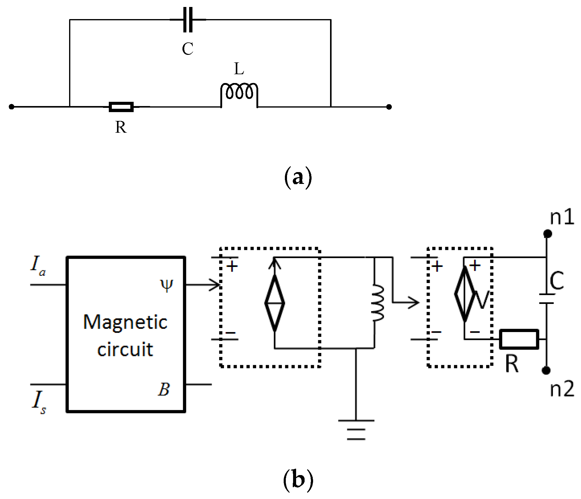
There are parasitic parameters in the magnetic part of the sensor, which should be taken into account in the simulation. The circuit with parasitic parameters for the magnetic core and coil is shown in Figure 4a. R and C are the parasitic resistance and capacitance of the coil, respectively, and the mutual inductance of the coil is described by the inductance, L.

The parasitic resistance and the parasitic capacitance can be calculated using the empirical formula. The electromagnetic induction effect of the coil inductance is equivalent to the time differential of the magnetic flux. The average magnetic flux in the magnetic core is computed as follows:

$$\begin{array}{l}\mathsf{\psi }=N{\displaystyle {\int }_{S}B·d\overrightarrow{S}}=\frac{N{\displaystyle {\int }_L{\displaystyle {\int }_{S}B·d\overrightarrow{S}}dl}}{L}=\frac{N{\displaystyle {\int }_L{\displaystyle {\int }_{S}B·}\widehat{t}dV}}{L}\\ =\frac{N}{L}{\displaystyle \sum _{m=1}^M{B}_m·{\overrightarrow{t}}_m\Delta V_m}\\ =\frac{N}{L}{\displaystyle \sum _{m=1}^M{\mathsf{\mu }}_0\left(M_m+H_m\right)·{\overrightarrow{t}}_m\Delta V_m}\end{array}$$

(19)

where L is the coil length, N is coil turns, M the number of tetrahedral elements of the magnetic core surrounded by the coil, $\widehat{t}$ is the unit tangential vector of the magnetic core, $\Delta V_m$ is the volume of the m-th tetrahedral element. $B_m$, $M_m$ and $H_m$ are, respectively, the magnetic induction strength, magnetization strength and magnetic field strength of the m-th tetrahedral element.

The voltage of the inductor in Figure 4a is obtained by the circuit in Figure 4b. The left part in Figure 4b is the magnetic component model in Section 3.3. The middle part in Figure 4b is the differential circuit, composed of a voltage-controlled current source and inductance. By calling upon the magnetic component model, the induced voltage V is obtained through the differential circuit. I_a is the measured current and I_s is the compensation coil current. B is the magnetic induction intensity at the air gap. $\mathsf{\psi }$ is the average magnetic flux.

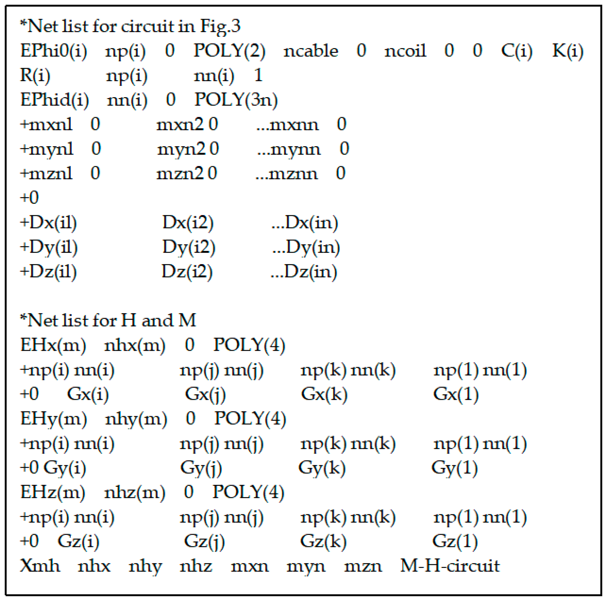
3.3. SPICE Netlist of Magnetic Circuit Model

One MSP-VIE sub-equation corresponds to one sub-circuit. The netlist for the sub-circuit corresponding to the i-th node (Figure 3) is shown in Figure 5. If the traditional method is applied to generate the netlist, a large circuit for n sub-equations (13) needs to be drawn in Workview. Through programming, using ‘ofstream’ head file and loop statements to change the node number, netlists for all sub-equations in (13) were written to the output file.

4. Fast Methods of Field–Circuit Combined Simulation

Compared with the simple equivalent models, the model in Section 3 considers the core structure, coil position and other factors in the equivalent circuit model, with the parameter matrices D, G, C, K in MSP-VIE regarded as the equivalent circuit parameters. At the same time, these many parameters also result in complicated models, and simulation-time consumption.

A well-established method in electromagnetic analysis, when symmetry exists, half, quarter or eighth models are widely used, to simplify the model and save computation time, because the number of elements is reduced. Another fast method has been developed, as follows:

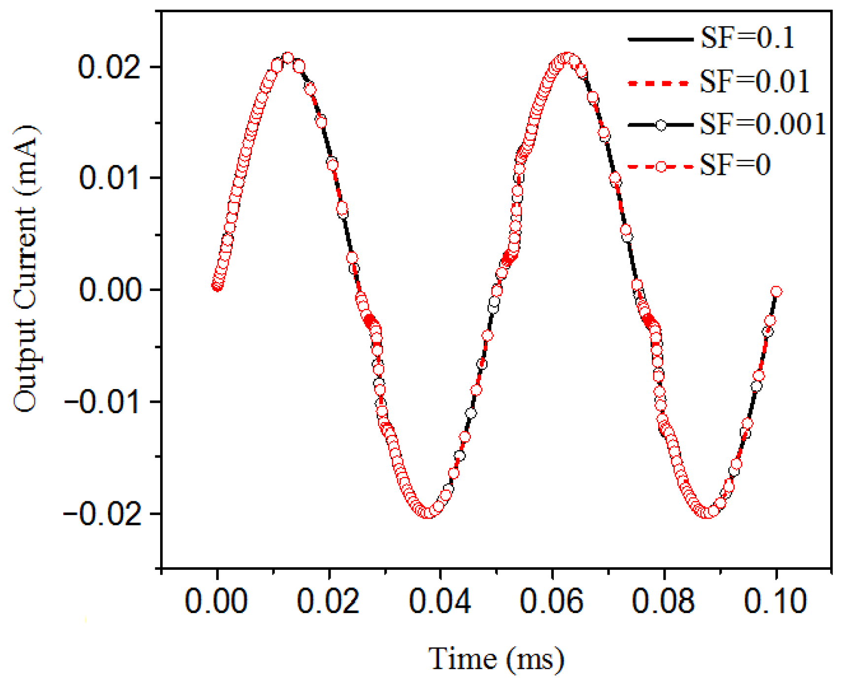
Because of the sparsity characteristic of the integral equation in the far area, there are a large number of small components in the corresponding matrix elements. The value of matrix elements represents the coupling relationship between sub-circuits, so it is feasible to utilize the matrix sparsity to reduce the circuit complexity and simplify the magnetic SPICE model.

The basic sparse strategy is ‘remove the small and preserve the big’, that is, to retain the large matrix elements and discard the small matrix elements. The size of the element value is judged by a sparse factor SF (man-made setting). If the ratio of the element in the $D$ matrix to the maximum value is greater than the SF, the element is retained, otherwise, the element is removed.

$$D=\left[\begin{array}{cccc}{D}_{11}& \cdots & D_{1j}& \cdots \\ ⋮& \ddots & ⋮& \\ D_{i1}& \cdots & D_{ij}& \cdots \\ ⋮& & ⋮& \end{array}\right] \{\begin{array}{l}SF>\left|\frac{D_{ij}}{D_{i\max }}\right|, \mathrm{removed}\\ SF\le \left|\frac{D_{ij}}{D_{i\max }}\right|, \mathrm{reserved}\end{array}$$

(20)

With symmetry in the magnetic field and matrix sparsity, the number of matrix parameters in the circuit is reduced; therefore, the SPICE model and netlist is simplified accordingly.

5. Numerical Example

5.1. Model Description

The detailed model for Figure 1 is shown below in Figure 6. R_m is the sampling resistance. The circuit between node n1 and node n2 is the magnetic core, with coil, which is described in Figure 4. According to the different application environments, the actual magnetic cores are various. This paper takes the silicon steel core shown in Figure 7 as an example, to test the proposed method. The outer diameter is 45 mm, the inner diameter is 35mm, the height is 5mm, and the air gap is 1.5 mm. The number of magnetic core meshes is 233. The number of compensation coil turns is 5000.

5.2. Simulation Results

Based on the SPICE model and netlist file, the joint simulation of the entire sensor can be implemented in SPICE.

Figure 8 is the experimental device. The current flowing through the feedback coil can be obtained by measuring the voltage of the sampling resistor R_m. Figure 9 shows the result (output current of the sensor) comparison between measurement and simulation, where the measured currents have different frequencies and amplitudes.

As shown in Figure 9, the proposed method can be used to carry out the field–circuit combined simulation for the sensor and obtain the transient output current for different measured input currents, which indicates that the method dynamically simulates the magnetic balance working process and gives the time-domain response. There are some differences between simulation and practice. This is because the parasitic capacitance of the coil is a distributed parameter, and it is not very accurate to use one capacitance description.

Figure 10 shows the simulation waveform for distortion analysis. As the frequency of the measured signal increases, the induced voltage increases and exceeds the power-supply voltage, resulting in n1 voltage peak shaving (Figure 10a). Coupled with the influence of parasitic capacitance, the current in the sampling resistor (Figure 10b) is distorted.

5.3. Fast Method Validation

Some numerical simulations were completed to evaluate the proposed fast method.

In the matrix sparsity method, the sparse factors were set as 0 (representing no sparse), 0.1, 0.01, and 0.001, respectively, for the SPICE simulation, and the measured current inputs were set as 100 A & 20 KHz. The results were as follows in Figure 11:

The comparison of simulation time under different sparse factors is displayed in the following

Table 1. Simulation consumption with different SF.

SF	SPICE Netlist Size (kb)	Simulation Time (s)
0.1	5047	620.06
0.01	16,836	3690.46
0.001	42,381	12,380.85
0	71,836	18,205.75

. The numerical results show that the matrix sparsity greatly improves the SPICE simulation speed, with high accuracy.

6. Conclusions

In this paper, a field–circuit combined simulation method, based on the magnetic scalar potential volume integral equation (MSP-VIE), is proposed, which discretizes the magnetic part of the sensor, by the electromagnetic field numerical method, and realizes field–circuit combination through solving the magnetic field equation in the circuit. The matrix extracted from MSP-VIE is put into the circuit as the equivalent circuit parameters of the magnetic part, and the magnetic scalar potential equation in the field is equivalent to the Kirchhoff voltage equation in the circuit, thus finishing the magnetic SPICE modeling. In addition, this paper presents a fast method with which to accelerate the SPICE simulation, which makes the method more convenient in practical applications.

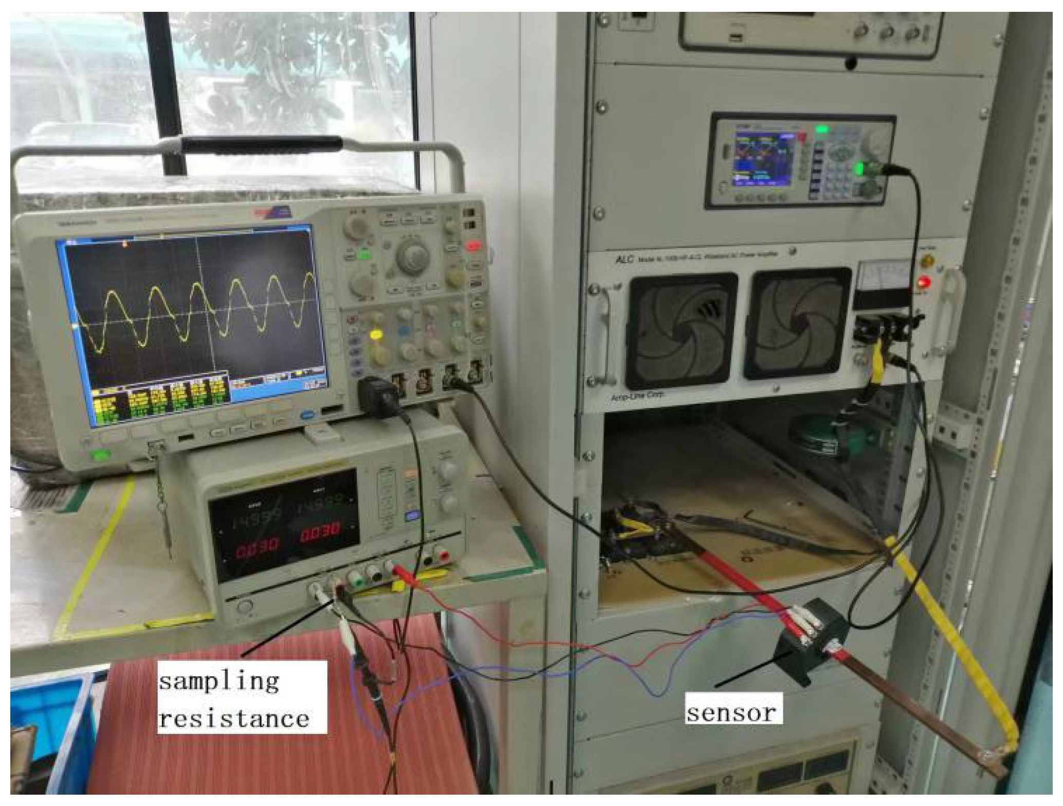
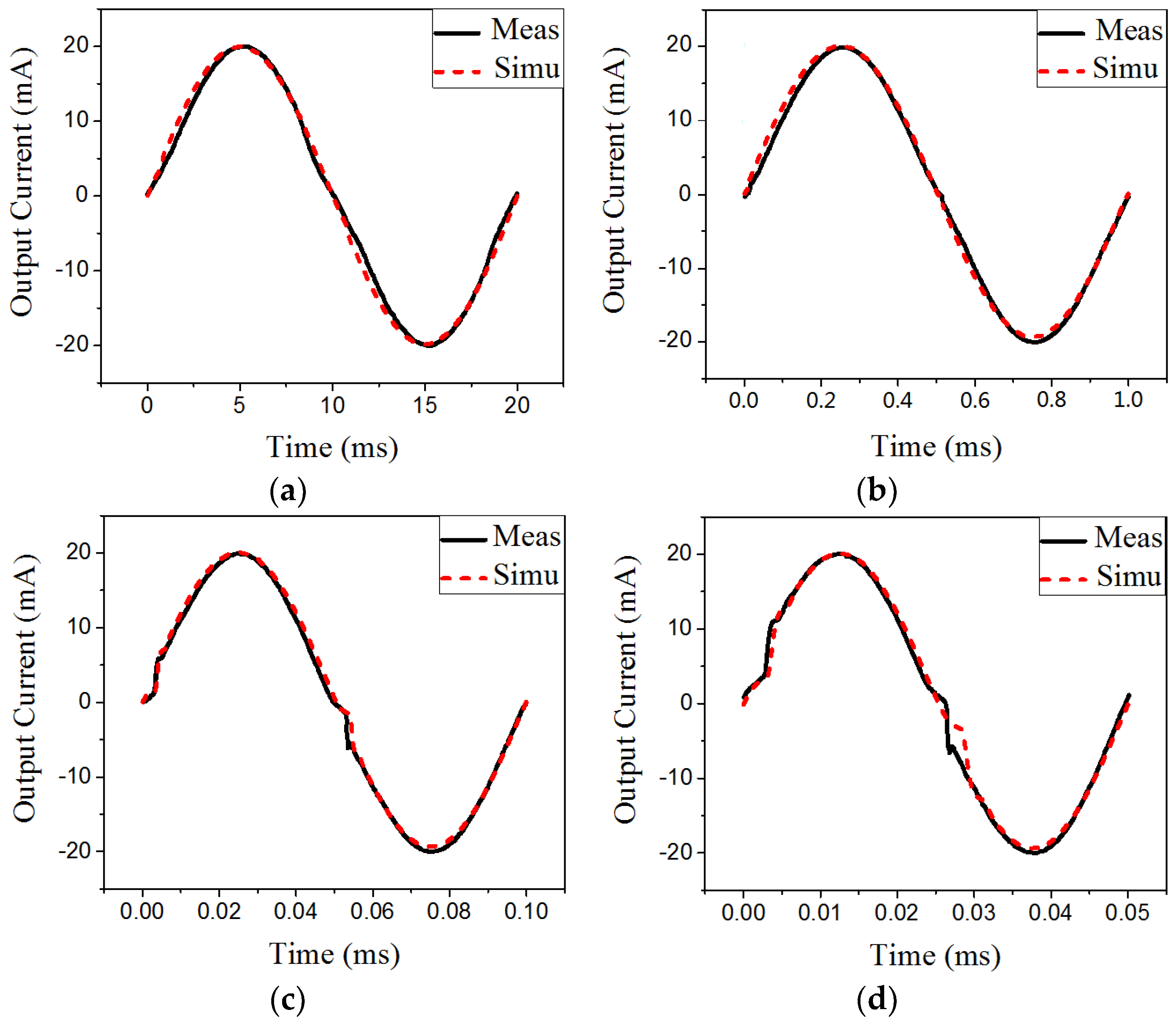
Simulation and measurement results reveal that this field–circuit combined method can dynamically simulate the working process of the magnetic balance current sensor and produce the time-domain transient response, as well as simulate some hidden performance details, by accurately considering the magnetic core. All of these factors make this method suitable for use in design, as well as product examination in practical engineering.