Local and Network Dynamics of a Non-Integer Order Resistor–Capacitor Shunted Josephson Junction Oscillators

Abstract

Spiral waves are an intriguing phenomenon that can be found in a variety of chemical and biological systems. We consider the fractional-order resistor–capacitor shunted Josephson junction chaotic oscillator to investigate the spiral wave pattern. For a preliminary understanding, we look at the dynamics of isolated FJJs and show that infinitely coexisting periodic and chaotic attractors depend on the fractional order. In addition, we perform bifurcation analysis to show the dynamical transition of the attractors as a function of fractional order and basin stability analysis to show the infinitely coexisting attractors. This is followed by the existence of spiral waves which is observed under various intrinsic and extrinsic system parameters. Finally, the impact of noise on SW is also analyzed by dispersing it to the entire stimulation period or defined time-period.

1. Introduction

Fractional-order (FO) systems can be found in many fields of science, including physics, electronics, biology, and engineering [1,2,3]. Hence, a wide range of studies have been conducted in recent years to better understand the dynamics of FO systems. From earlier reports, it has been revealed that fractional order (non-integer order) systems can more effectively mimic the real-time dynamics than integer order systems [1,2]. In addition, researchers have discovered that FO models are the most effective tool for examining memory effects and the genetic characteristics of biological systems [4,5,6]. Furthermore, the FO calculus can improve the accuracy and flexibility of computations and has applications in computation optimization and control performance [6,7,8]. As a result, there has been an increase in interest in studying FO-induced dynamical behaviors in recent years; many nonlinear systems can be modeled and studied as FO systems. Synchronization and chimera have been observed in FO neurons, including Hindmarsh–Rose (HR) and FitzHugh–Nagumo (FHN) neurons, depending on the fractional derivative and coupling strength [9,10,11]. Various spiking and bursting patterns have been reported using the realistic biological Izhikevich model [12]. Furthermore, under electromagnetic radiation, adaptive synchronization has been observed in FO HR neurons [13]. The occurrence of synchronization has also been demonstrated by extending the multiplex FO network [14].

On the other hand, the Josephson junction is a critical component in superconducting electronics (SCE) that is typically developed by separating two superconductors by extremely thin non-superconducting layers [15]. Due to the thin insulating barrier, the electrons could easily travel from one superconducting layer to the next. This is known as Josephson tunneling [16]. Since then, the JJ has had a wide range of applications in implementing SCE devices in advanced technologies [17]. As a result, the JJ plays a crucial role in employing the different SC devices including SQUIDS, superconducting qubits, radiation detectors, rapid single flux quantum (RSFQ), a digital electronic device, etc. [18,19,20,21]. In addition, based on the application, several kinds of JJ have been implemented which include resistively shunted junctions (RSJ), resistive and capacitive shunted junctions (RCSJ), resistive-capacitive-inductance shunted junctions (RCLSJ), and periodically modulated Josephson junctions (PMJJ) (PMJJ). Originally, the existence of chaos and intermittent chaos was demonstrated using RSJ [22,23,24]. Subsequently, the periodic-to-chaotic transition and coexisting chaotic attractor with phase-locking conditions were reported using a RCSJ [25,26]. This has been followed by the synchronization and control of chaos which were achieved using nonlinear-RCLSJ with DC bias [27,28]. Eventually, distinct slow–fast dynamics have been detected when replacing the nonlinear resistance with linear resistance [29]. The significance of a commensurate fractional derivative was investigated using FO chaotic no equilibrium linear-RLCSJ and demonstrated synchronization with applications in digital cryptography [30].

In addition to the foregoing, the spiral wave is a remarkable spatiotemporal pattern compared to the other dynamical behaviors [31,32,33,34] found in many excitable chemical and biological systems [35,36,37,38,39]. The spiral wave pattern was first detected in the Belousov–Zhbotinsky (RZ) reactions [40]. Subsequently, the investigation of the spiral waves has received increasing attention over the years. As a result, it has been studied in a variety of map-lattices, neuronal systems, chaotic systems, and many other systems [41,42,43]. For instance, the formation of different spiral wave patterns such as periodic, banded, and domain patterns has been discovered using a 2D lattice of sine-circle maps [44]. Furthermore, the spiral wave chimera where the occurrence of asynchronous behavior at the core of the ordered spiral waves has been realized in a large population of chemical oscillators [45]. Such spatio-temporal patterns were also observed in nonlocally coupled Fitzhugh–Nagumo systems [46], as well as regular and fractal adaptive exponential integrate-and-fire (AEIF) neurons [47]. As a result of the inter-layer coupling interaction, the multilayer networks of the Fitzhugh–Nagumo neural networks also exhibit a spiral wave in one layer and a homogeneous state in the other layer [48]. Furthermore, the occurrence of spiral waves has also been demonstrated using an FO discrete neuron map and memristor-based hyperchaotic system [49,50]. Furthermore, the suppression mechanism for the spiral waves has been described using impulse triggering [50]. Motivated by the aforementioned findings, we investigate the dynamics and properties of the FO resistor–capacitor shunted Josephson junction chaotic oscillator. Furthermore, the emergence of spiral waves in FO JJ is still unknown and has not been thoroughly investigated in FJJ. To do so, we examine whether the lattice network FJJ can exhibit a spiral wave pattern. If so, what are the influences of other parameters such as external stimulus amplitude and coupling strength? To respond to the foregoing, the dynamics of the FJJ are examined, and it is discovered that the local dynamics exhibit infinitely coexisting periodic and chaotic attractors. We also show that, depending on the fractional-order and coupling strength, network dynamics can exhibit a spiral wave pattern.

Furthermore, noise is ubiquitous and can inevitably exist in many practical systems [51,52]; a wide range of studies have been conducted in the literature to explore the impacts of noise in dynamical systems. In particular, state-dependent noise is used to suppress chaos in fractional order chaotic systems [53]. Furthermore, noise-induced and enhanced complete synchronization were found in FO chaotic systems [54]. It has been shown that noise can enhance the oscillatory behavior of FO parametrically driven nonlinear systems [55]. We analyze the influence of noise in FJJO by giving it during a fixed time period and the entire simulation time period to study the impact of noise on spiral waves because of its importance in FO systems.

The remaining sections of the article are as specified: Section 2 introduces the proposed model of FJJ oscillators. Section 3 discusses the dynamical behaviors of the considered FJJ using bifurcation analysis. Furthermore, the infinite coexistence of periodic and chaotic attractors is illustrated using a basin of attraction. The corresponding network dynamics of FJJ are detailed in Section 4. We specifically explore the influence of various parameters such as external force amplitude, coupling strength, and d on the occurrence of spiral wave patterns. Subsequently, we address the influence of Box–Muller noise on SW by dispersing it throughout the whole simulation period or a specified time-period in Section 5. Finally, the findings will be summarized in Section 6.

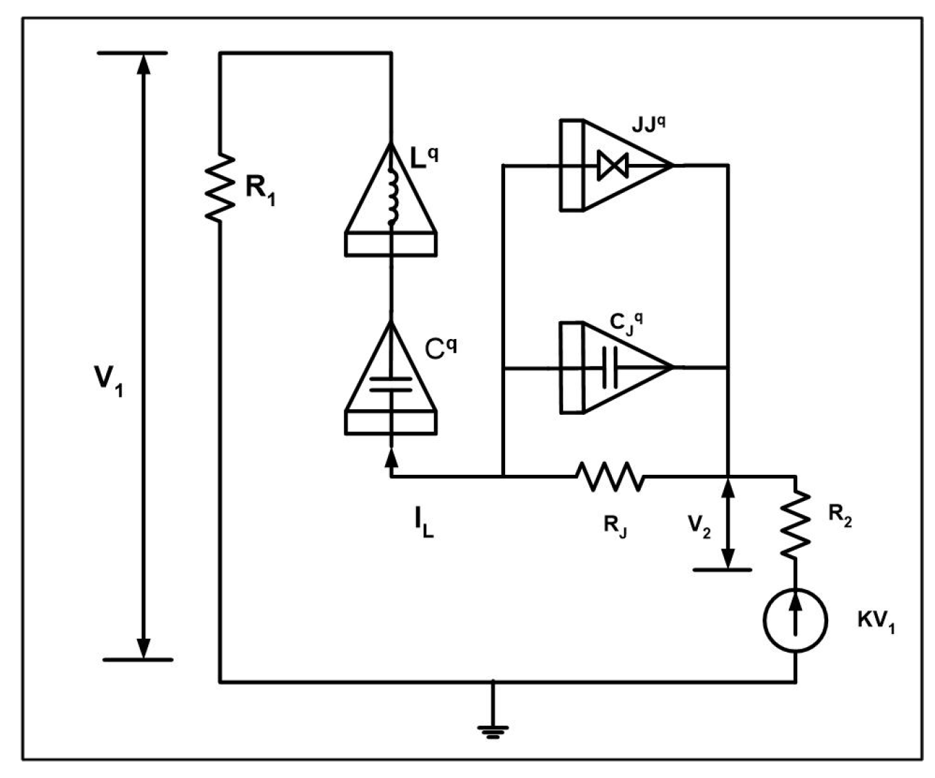
2. Fractional-Order JJ Oscillator (FJJO)

In [56], the authors discussed a simple autonomous chaotic oscillator with a Josephson junction resonator and an inductor, a capacitor, and an amplifier. The authors have shown the various dynamical properties of the oscillator and interestingly, the oscillator exhibits multiple coexisting attractors. It should be noted that the oscillator in [56] is an integer order circuit, but as it was in [57], the authors have shown the effectiveness of the fractional order analysis of circuits with electrical components such as active semiconductor devices, capacitors, and inductors. Hence, we investigate the fractional-order model of the oscillator in Figure 1, and we have shown the modified circuit with fractional-order capacitor and inductor [58] along with a fractional-order Josephson junction resonator.

Applying KCL and KVL to the circuit shown in Figure 1 and by considering the phase difference between the semiconductor in the FJJ, voltage across the FJJ, voltage across the capacitor and current through the inductor as the four states, the dynamical equations are derived as

$$\begin{array}{ccc}\hfill \frac{d^{q}x}{d{t}^q}& =& V_J,\hfill \\ \hfill C_J^q\frac{d^q{V}_J}{d{t}^q}& =& I_L-\frac{V_J}{R_J}-I_{J}sin\left(x\right),\hfill \\ \hfill C^q\frac{d^q{V}_c}{d{t}^q}& =& I_L,\hfill \\ \hfill L^q\frac{d^q{I}_L}{d{t}^q}& =& ((K-1)R_1-R_2)I_L-(V_J+V_c).\hfill \end{array}$$

(1)

To derive the dimensionless model of (1), we use the states as $V_j=y,V_c=z,I_L=C_J^{q}w$ and the parameters as $a=\frac{I_c}{C_j^q}$, $b=\frac{C_j^q}{C^q}$, $c=\frac{-((K-1)R_1-R_2)}{L^q}$, $d=\frac{1}{C_j^q{L}^q},\alpha =\frac{1}{R_j{C}_j^q}$. Using these assumptions, the dimensionless model of (1) is derived as

$$\begin{array}{ccc}\hfill \frac{d^{q}x}{d{t}^q}& =& y,\hfill \\ \hfill \frac{d^{q}y}{d{t}^q}& =& w-\alpha y-asin\left(x\right),\hfill \\ \hfill \frac{d^{q}z}{d{t}^q}& =& bw,\hfill \\ \hfill \frac{d^{q}w}{d{t}^q}& =& cw-d(y+z),\hfill \end{array}$$

(2)

From Equation (1), we consider the parameters as defined in Equation (3) for our simulations unless otherwise specified.

$$\alpha =1.18,a=0.25,b=0.08,c=0.17,d=0.31.$$

(3)

The initial value problem of system (2) is achieved using the predictor–corrector scheme of the Adams–Bashforth–Moulton (ABM) method [59,60] In order to do so, we consider a generalized form of the FO differential equation, which can be written as

$$\begin{array}{c}\hfill D^{q}u\left(t\right)=f(t,u\left(t\right)),0\le t\le T,\end{array}$$

(4)

where $u^j\left(0\right)$ = $u_0^j$, $j=0,1,...,⌈q⌉-1$. The solution of Equation (4) can be written as a Volterra integral form, as given below

$$\begin{array}{c}\hfill u\left(t\right)=\sum _{j=0}^{⌈q⌉-1}{u}_0^j\frac{t^j}{j!}+\frac{1}{\mathrm{\Gamma }q}{\int }_0^1\frac{f(\tau ,u)}{{(t-\tau )}^{1-q}}d\tau .\end{array}$$

(5)

The numerical solution of Equation (4) is obtained for with $n=0,1,2,...,N$. N is an integer and h is the stepsize $h=T/N$. The discrete form of Equation (5) for the corrector is obtained as

$$\begin{array}{c}\hfill u_h\left(t_{n+1}\right)=\sum _{N=0}^{q-1}{u}_0^N\frac{t^N}{N!}+\frac{h^q}{\mathrm{\Gamma }q+2}f(t_{n+1},u_h^p\left(t_{N+1}\right))+\frac{h^q}{\mathrm{\Gamma }(q+2)}\sum _{k=0}^n\left(a_{k,n+1}f(t_k,u_h\left(t_k\right))\right),\end{array}$$

(6)

where

$$\begin{array}{c}\hfill a_{k,n+1}=\left\{\begin{array}{cc}{n}^{q+1}-(n-q){(n+1)}^q,\hfill & k=0,\hfill \\ {(n-k+2)}^{q+1}+{(n-k)}^{q+1}-2{(n-k+1)}^{q+1},\hfill & 1\le k\le n,\hfill \\ 1,\hfill & k=n+1.\hfill \end{array}\right.\end{array}$$

(7)

Furthermore, the predictor can takes the form

$$\begin{array}{c}\hfill u_h^p\left(t_{n+1}\right)=\sum _{j=0}^{n-1}{u}_0^j\frac{t^j}{j!}+\frac{1}{\mathrm{\Gamma }q}\sum _{k=0}^n{b}_{k,n+1}f(t_k,u_h\left(t_k\right)),\end{array}$$

(8)

where $b_{k,n+1}$ is obtained as

$$\begin{array}{c}\hfill b_{k,n+1}=\frac{h^q}{q}{((n+1)-j)}^q-(n-k^q).\end{array}$$

(9)

The system variables of Equation (2) are discretized using Equations (6)–(8) to obtain the numerical solutions.

3. Dynamical Behavior and Its Transitions of FJJO

The dynamical behavior of the system (2) is investigated in the following subsections using phase portrait trajectory, bifurcation analysis, and basin stability analysis.

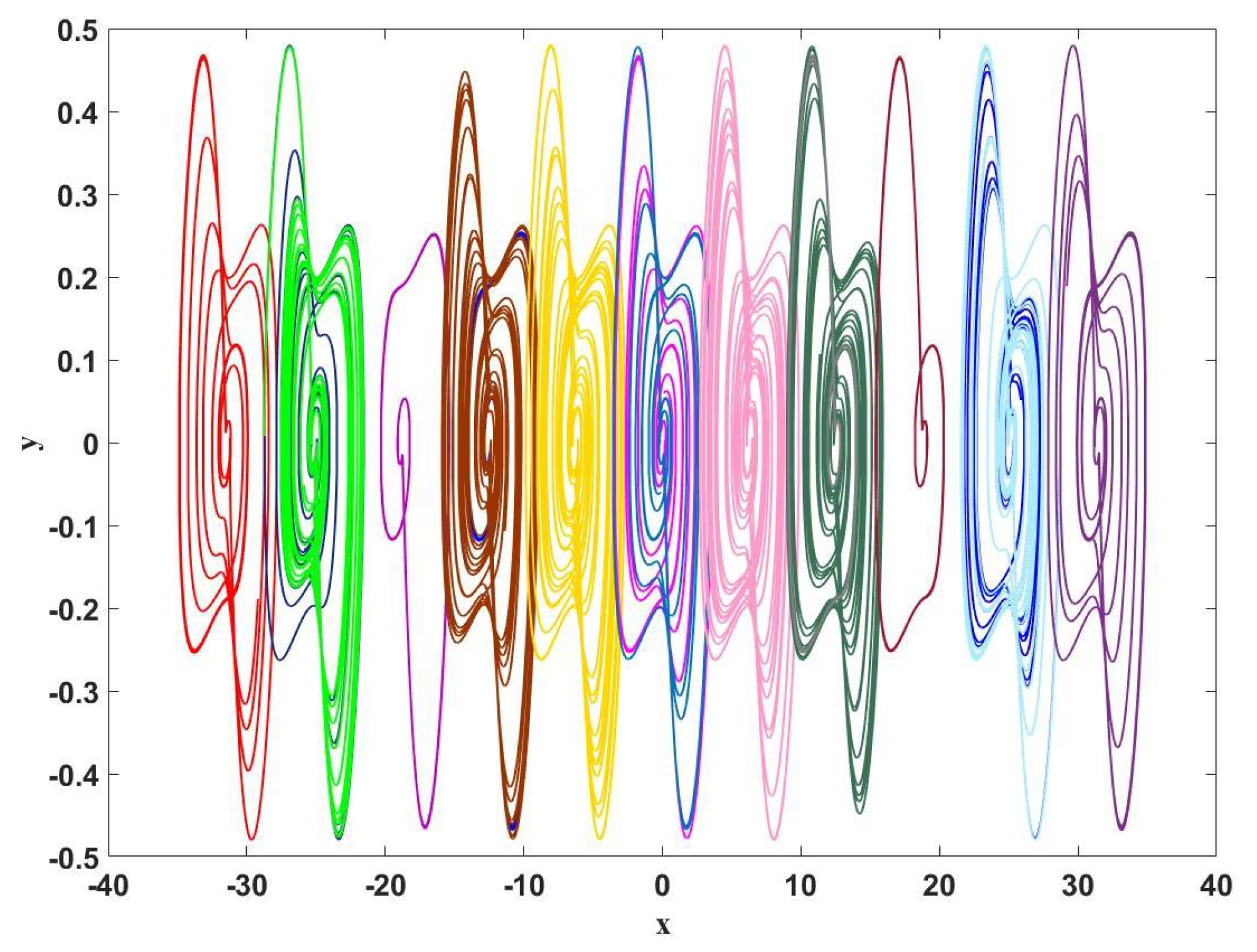
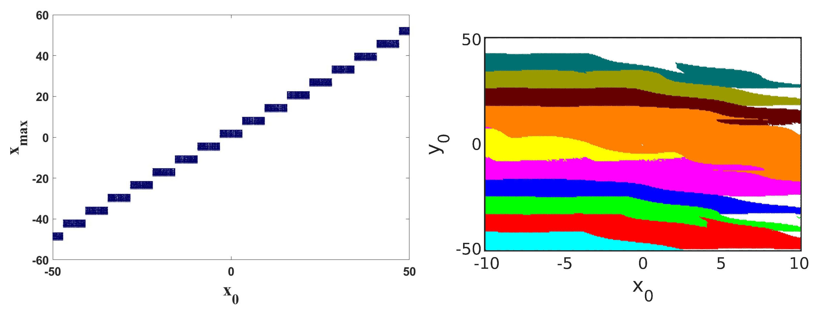
3.1. Infinitely Coexisting Periodic and Chaotic Attractors

For a primary understanding of the dynamical behavior of FJJO, we plotted the phase portrait trajectory of the observed attractors in Figure 2 by fixing the FO as $q=0.98$. It is noticeable that the ($x,y$) plane has infinitely many attractors. Distinct colors represent different attractors for various initial conditions. We observed a few periodic attractors coexisting with chaotic attractors, while prior studies have shown that chaotic attractors can coexist with torus attractors alone [61,62]. As a result, the coexistence of periodic and chaotic attractors that we observed here is interesting and has yet to be reported in the literature.

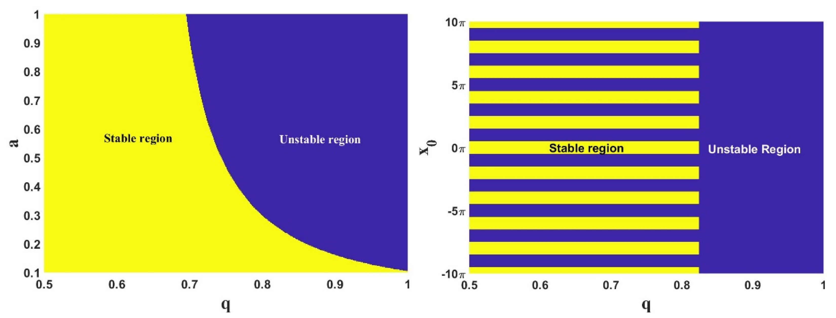
3.2. Stability of the Equilibrium Points

To determine the stability, we find the equilibrium points that correspond to Equation (2), which is given as $E=({sin}^{-1}\left(0\right),0,0,0)$ where ${sin}^{-1}\left(0\right)=n\pi$ and n is an integer. The obtained fixed points imply the existence of an infinite number of equilibrium points. The observed equilibrium points are stable when the following criterion is satisfied.

$$\begin{array}{c}\hfill |arg\left({\lambda }_j\right)|>\frac{q\pi }{2},j=1,2,3,...\end{array}$$

(10)

where $\left({\lambda }_j\right)j\in 1,4$ are the eigenvalues of the characteristic equation $det\left(diag\right({\lambda }_1^q,{\lambda }_1^q,$${\lambda }_2^q,{\lambda }_3^q,{\lambda }_4^q)-J_E)=0$, where q is the commensurate fractional-order and $J_E$ is the Jacobian at the equilibrium point. Using the above condition (given in Equation (9)), we demarcated the stability region by varying the parameter a and initial state $x_0$ with respect to the fractional-order q in Figure 3. In ($q,a$) space, the increasing stability area while the parameter a reduces is noticeable. As illustrated in Figure 3 (left plot), the occurrence of stable and unstable regions switches depending on the value of $x_0$, and it becomes fully unstable beyond a certain fractional order threshold.

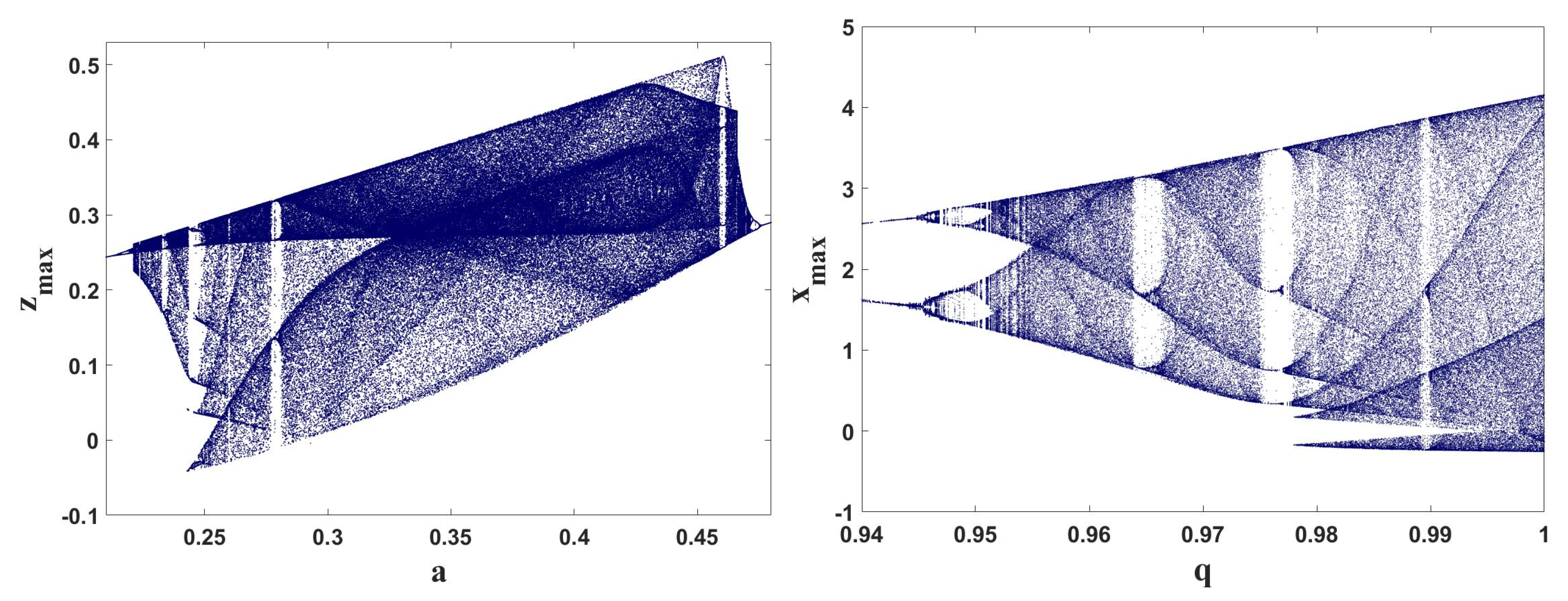
3.3. Dynamical Transitions through Bifurcation Analysis

Furthermore, the dynamical transitions of FJJO are analyzed through a one-parameter bifurcation diagram using the local maxima of the variables as illustrated in Figure 4. Firstly, the $z_{max}$ is portrayed as a function of a in Figure 4. When increasing the magnitude of a, we can observe the transition from periodic to chaotic through the period doubling (PD) route (see right plot). Following that, the one-parameter bifurcation diagram is plotted by varying the fractional order q and finding the local maxima of the x variable in Figure 4 (left plot). It is clear that increasing fractional-order leads to a chaotic attractor from periodic attractor via period-doubling.

The bifurcation diagram is shown by varying the initial state of the x-variable (i.e., $x_0$), to demonstrate the infinitely coexisting attractors. The attractor basin is obtained by providing the chosen range of the initial state as an equilibrium point of a variable. The shifting of the attractor basins as a function of the initial states is evident from Figure 5 (left plot). For a more clear understanding of the coexisting attractors, we plotted the basin of attraction by varying the initial state of $x_0$ and $y_0$. Depending on the initial state values of $x_0$ and $y_0$, the basins of each attractor shift from one attractor to the other as shown in Figure 5 (right plot). As a result, the coexistence of infinite attractors based on the initial states is evident in Figure 5.

From the observation, it is clear that the isolated FJJO can produce infinitely coexisting periodic and chaotic attractors with respect to the fractional orders. The dynamical behavior of the FJJO network is further discussed below by extending it to a two-dimensional array.

4. Network of FJJ and Its Collective Dynamics

In addition, we extend our analysis to the network FO-resistor–capacitor shunted Josephson junction, and the corresponding dynamical equation for a two-dimensional array of FJJ with nearest-neighbor interaction can be written as

$$\begin{array}{ccc}\hfill \frac{d^q{x}_{i,j}}{d{t}^q}& =& y_{i,j}+G\left(t\right){\beta }_{ij}+D(x_{i+1,j}+x_{i-1,j}+x_{i,j+1}+x_{i,j-1}-4x_{i,j})+\eta \left(t\right)\hfill \\ \hfill \frac{d^q{y}_{i,j}}{d{t}^q}& =& w_{i,j}-\alpha y_{i,j}-asin\left(x_{i,j}\right),\hfill \\ \hfill \frac{d^q{z}_{i,j}}{d{t}^q}& =& b{w}_{i,j},\hfill \\ \hfill \frac{d^q{w}_{i,j}}{d{t}^q}& =& c{w}_{i,j}-d(y_{i,j}+z_{i,j}).\hfill \end{array}$$

(11)

Here, we considered the 2D lattice network with $i,j=1,2,...,N$—where N is the number of nodes in a lattice array that can take the value $N=100$. D is the coupling strength. $\eta \left(t\right)$ is the Box–Muller noise defined as $\eta \left(t\right)=\left(\frac{-4\delta }{\Delta t}ln\left(c_1\right)\right)0.5cos\left(2\pi c_2\right)$ where $c_1$ and $c_2$ are randomly chosen between $[0,1]$, $\delta$ is the variance of the noise and $\Delta t$ is the step size.$G\left(t\right)=Asin\left(\omega t\right)$, which represents external periodic stimuli, is applied at the center of the node. If $i=j=75$ then ${\beta }_{ij}=1$, the periodic stimulus is applied, otherwise ${\beta }_{ij}=0$, and the periodic stimulus is not applied. Here $\omega$ denotes the frequency of the external stimuli, which is set to $\omega =0.001$. The collective dynamical behavior of the system (4) is explored by computing the energy of each node in the lattice network, as detailed below.

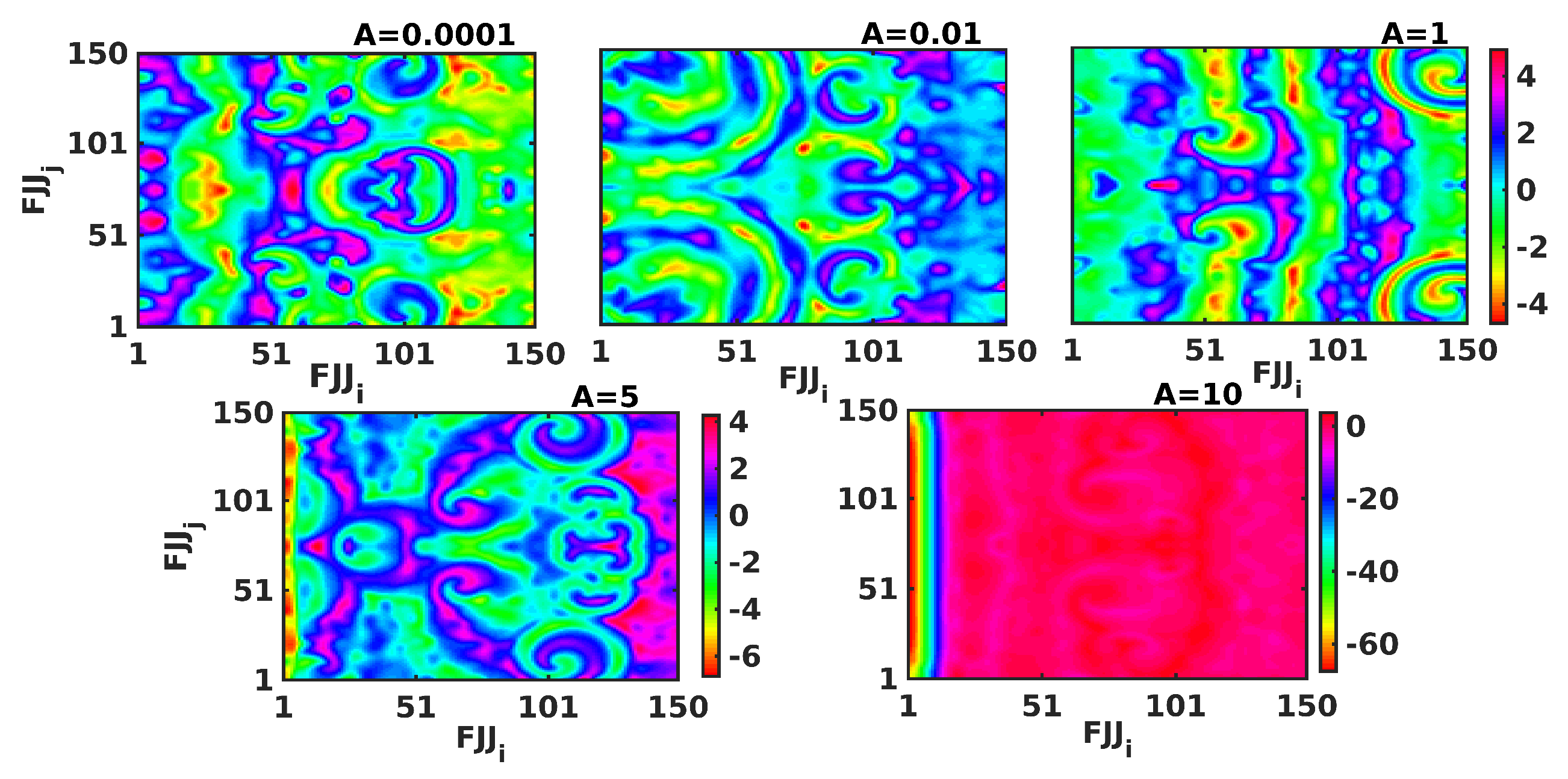
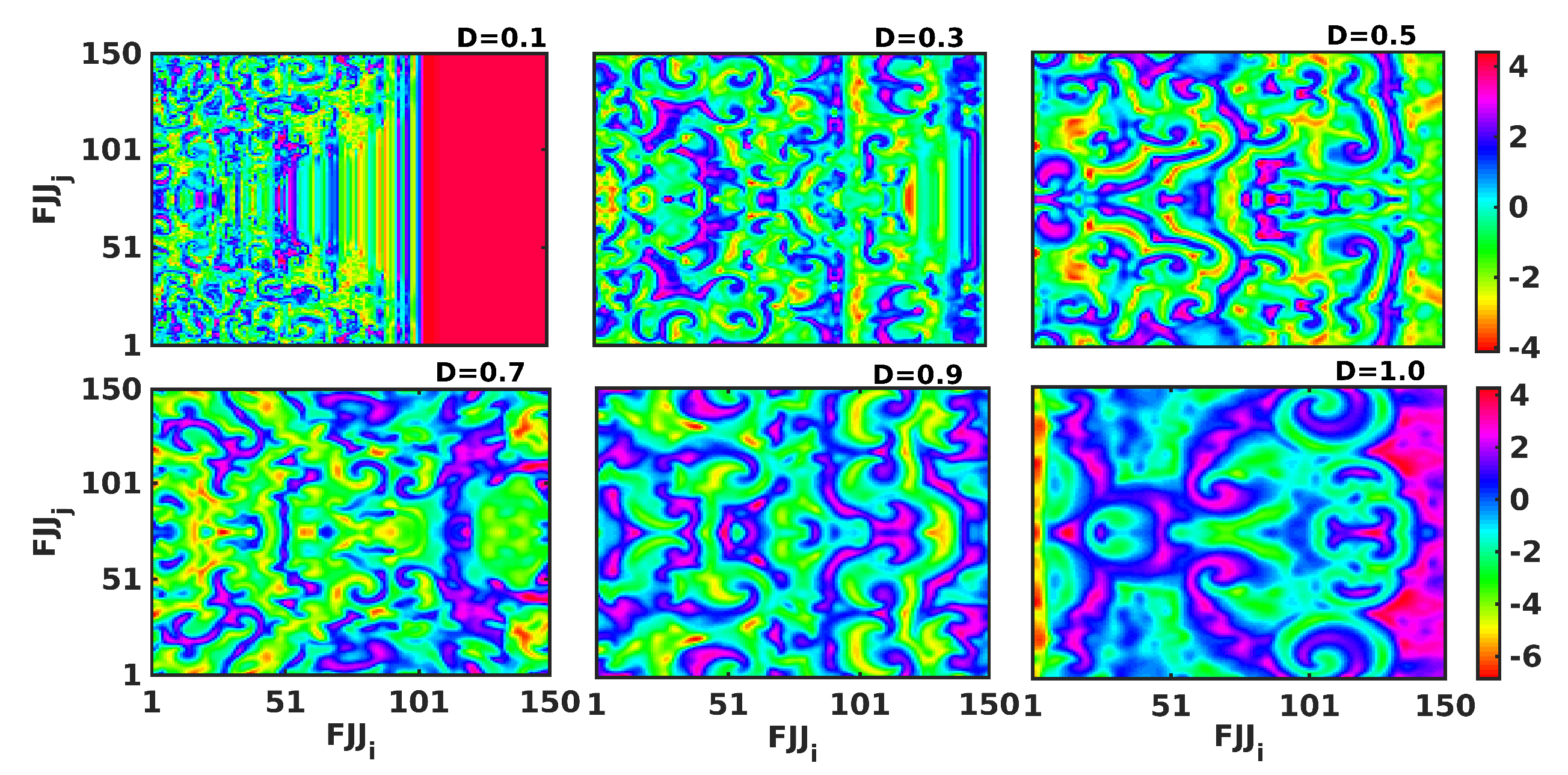
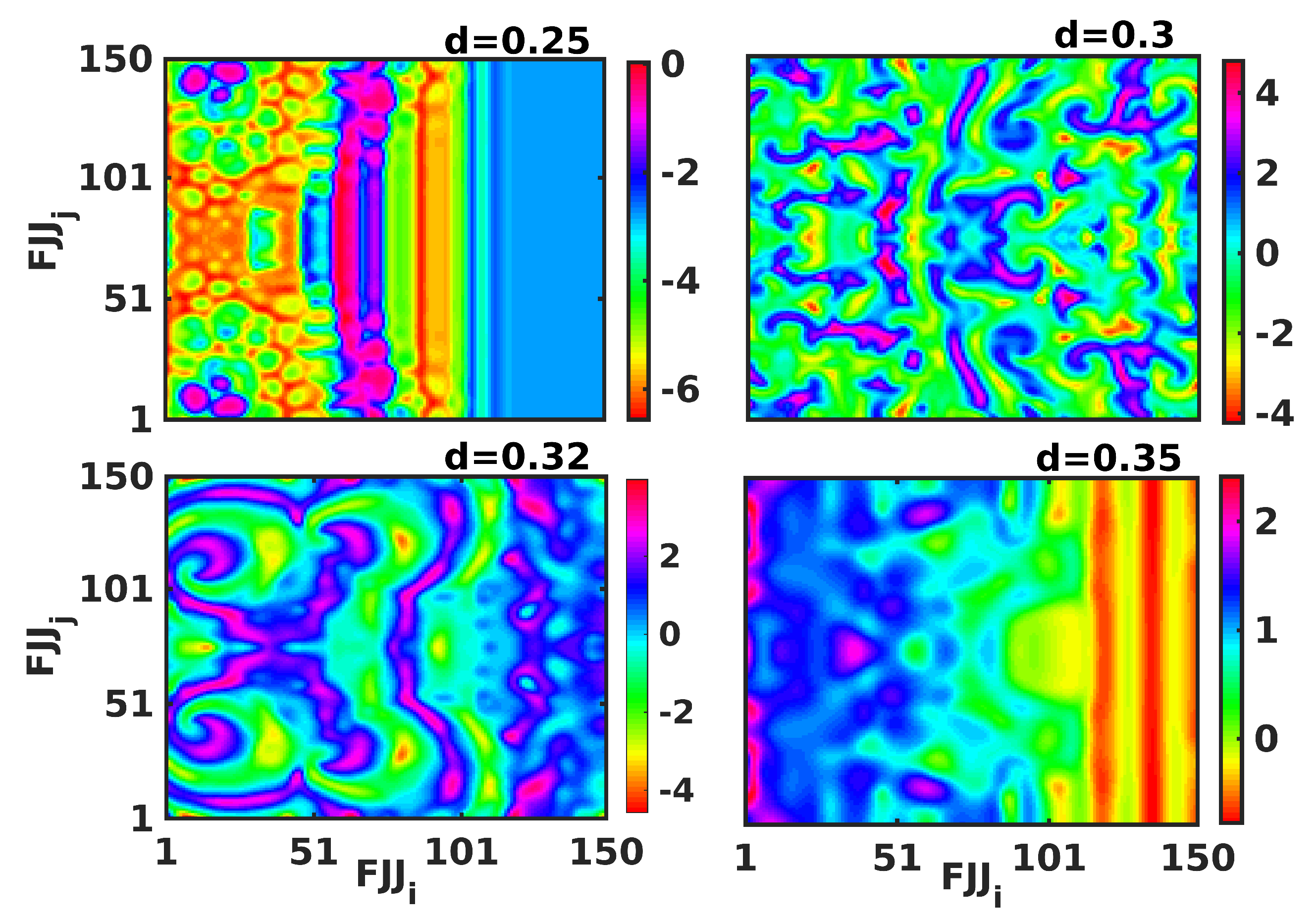
Impact of Distinct Intrinsic and Extrinsic Parameters in a Network of FJJ

We first demonstrate the formation of spiral wave patterns in a network of FJJ by determining the energy of each node for different values of external stimulus amplitude (A) in Figure 6. For $A=0.001$, it is evident that the nodes are in lower and higher intensities. Such heterogeneity in energy levels confirms the presence of SW. Analogously, SW patterns can also be noticed when A is increased to $A=0.01$, $A=1.0$, and $A=5.0$. If the amplitude of external forcing is raised to $A=10$, all the nodes experience lesser intensity due to energy dissipation. As a result, we witnessed SW disappear with lesser intensity plane waves.

We exemplified the energy of each node in Figure 7 by setting different coupling strengths to explore the influence of coupling strength on the occurrence of the SW. If the coupling strength is minimal for $D=0.1$, the energy spread occurs just in a portion of the array of nodes, while the remaining remains at rest. As a result, the partial nodes exhibit the SW pattern while the other nodes are in the rest state. Furthermore, we can observe the spread of dynamics over the entire array while the coupling strength is increased to $D=0.3$. As the coupling strengths are raised to $D=0.5,0.7$, and $0.9$, a spiral wave with several arms appears. Furthermore, we discovered a more prominent spiral wave pattern when the coupling strength is increased to $D=1.0$.

The dynamical behavior of the system (4) is further examined by changing the value of d in Figure 8. When $d=0.25$, we determined that the onset of SW occurs with heterogeneous lower intensity nodes, while the remaining nodes are in a lower intensity rest state, implying that the energy is dispersed across just a portion of the nodes. A spiral wave with multiple arms arises when the parameter value is raised to $d=0.3$. At $d=0.35$, increasing the value of d further decreases the arms and generates turbulent behavior. Under turbulent conditions, a low-intensity traveling wave can also be detected.

5. Impact of Box–Muller (BM) Noise in a Network of FJJ

In the following, we looked at the influence of BM noise [51,52] on observed SW in the array of FJJ by distributing it in two distinct ways. Firstly, the behavior of the network is analyzed by distribution noise throughout the simulation time. Subsequently, the noise is applied only between 500–700 s times. The observed outcomes are described in detail below.

5.1. Noise Applied for the Entire Simulation Time Period

The influence of noise is investigated by setting the parameter at SW and fixing different values of the variance of BM noise. At extremely low variance values, $\delta =0.0001$, there is not much effect on SW behavior. Furthermore, the SW retains its behavior when the variance is raised to $\delta =0.01$, $\delta =0.1$, and $\delta =1$. When the BM noise variation is raised further, a spiral wave with multiple arms forms for $\delta =5$. At larger variance $\delta =10$, the spiral waves are suppressed, resulting in the creation of two different zones with varying intensities. The first zone has nodes with greater intensities than the second zone, which comprises nodes with lower intensities shown in Figure 9.

5.2. Noise Applied for a Specific Time Period between 500 and 700 s

In addition, we examined the influence of noise on the SW pattern by applying the noise only for a defined time period of $500–700 \mathrm{s}$, as compared to the earlier research, in which the noise was distributed throughout the simulation. Figure 10 strongly demonstrates that a spiral wave exists for the noise variance $\delta =0.0001$ and $\delta =0.001$. The number of arms in the spiral waves increased when the variance is increased to $\delta =0.01$, resulting in multi-arm spiral waves. We also noted that the suppression of SW as the variance is increased to $\delta =0.03$. Furthermore, the lattice array shows two distinct zones for $\delta =0.05$, one with high-intensity nodes and the other with low-intensity nodes.

Based on the observations, it is clear that the considered FJJ can exhibit neuron-like dynamics in the form of a coexisting periodic and chaotic attractor as well as a spiral wave pattern depending on various factors such as fractional-order, coupling strength, amplitude of external periodic external stimuli, and noise intensity.

6. Conclusions

In this study, we considered the fractional-order resistor–capacitor shunted Josephson junction to investigate the local and network dynamics with respect to the fractional-order. We discovered that the considered system has infinitely coexisting chaotic attractors interspersed with a few periodic attractors depending on the FO. Furthermore, the dynamical transitions of the attractors were investigated using bifurcation analysis, and the existence of infinitely coexisting attractors was validated using a basin of attraction. As a function of fractional order, the bifurcation transition portrayed the transition from periodic attractor to chaotic attractor via period-doubling route. More significantly, we extended the study to the FJJ network by considering the $2D$ lattice array of JJ and demonstrated the influence of several parameters such as amplitude external forcing, coupling strength, and d. We found that the formation of spiral waves by fixing different values of the amplitudes of external stimulus (A) which suppresses further when increasing A to larger values. We also identified that the sufficient strength of coupling strength and the magnitude of d was essential for the formation of SW over the entire nodes in the lattice. Finally, the impact of BM noise was addressed by employing it in two distinct ways. First, the SW dynamics were investigated by dispersing noise throughout the simulation. It was further examined by dispersing it at specific time intervals. By comparing the two cases, it was shown that providing noise just for a specific time interval can suppress the SW at lower noise variance values than applying noise throughout the whole simulation, which suppresses the SW at higher magnitudes of variance. Thus, we believe that the obtained results may shed light on the dynamics of JJ in superconducting electronic devices, particularly in the implementation of superconducting quantum computing and superconducting switching devices.

References

1. Akdemir, A.O.; Dutta, H.; Atangana, A. Fractional Order Analysis: Theory, Methods and Applications; John Wiley & Sons: New York, NY, USA, 2020. [Google Scholar]
2. Kilbas, A.A.; Srivastava, H.M.; Trujillo, J.J. Theory and Applications of Fractional Differential Equations; Elsevier: Amsterdam, The Netherlands, 2006. [Google Scholar]
3. Yu, C.H. Fractional derivatives of some fractional functions and their applications. Asian J. Appl. Sci. Technol. 2020, 4, 147–158. [Google Scholar] [CrossRef]
4. Si, L.; Xiao, M.; Jiang, G.; Cheng, Z.; Song, Q.; Cao, J. Dynamics of fractional-order neural networks with discrete and distributed delays. IEEE Access 2019, 8, 46071–46080. [Google Scholar] [CrossRef]
5. Kaslik, E.; Sivasundaram, S. Dynamics of fractional-order neural networks. In Proceedings of the 2011 International Joint Conference on Neural Networks, San Jose, CA, USA, 16–22 July 2011; pp. 611–618. [Google Scholar]
6. Jacob, J.S.; Priya, J.H.; Karthika, A. Applications of fractional calculus in science and engineering. JCR 2020, 7, 4385–4394. [Google Scholar]
7. Liu, H.; Li, S.; Cao, J.; Li, G.; Alsaedi, A.; Alsaadi, F.E. Adaptive fuzzy prescribed performance controller design for a class of uncertain fractional-order nonlinear systems with external disturbances. Neurocomputing 2017, 219, 422–430. [Google Scholar] [CrossRef]
8. Das, S. Functional Fractional Calculus; Springer: Berlin, Germany, 2011. [Google Scholar]
9. Ramadoss, J.; Aghababaei, S.; Parastesh, F.; Rajagopal, K.; Jafari, S.; Hussain, I. Chimera state in the network of fractional-order fitzhugh–nagumo neurons. Complexity 2021, 2021, 2437737. [Google Scholar] [CrossRef]
10. Vázquez-Guerrero, P.; Gómez-Aguilar, J.F.; Santamaria, F.; Escobar-Jiménez, R.F. Synchronization patterns with strong memory adaptive control in networks of coupled neurons with chimera states dynamics. Chaos Solitons Fractals 2019, 128, 167–175. [Google Scholar] [CrossRef]
11. He, S. Complexity and chimera states in a ring-coupled fractional-order memristor neural network. Front. Appl. Math. Stat. 2020, 6, 24. [Google Scholar]
12. Teka, W.W.; Upadhyay, R.K.; Mondal, A. Spiking and bursting patterns of fractional-order Izhikevich model. Commun. Nonlinear Sci. Numer. Simul. 2018, 56, 161–176. [Google Scholar] [CrossRef]
13. Meng, F.; Zeng, X.; Wang, Z.; Wang, X. Adaptive synchronization of fractional-order coupled neurons under electromagnetic radiation. Int. J. Bifurc. Chaos 2020, 30, 2050044. [Google Scholar] [CrossRef]
14. Ramakrishnan, B.; Parastesh, F.; Jafari, S.; Rajagopal, K.; Stamov, G.; Stamova, I. Synchronization in a Multiplex Network of Nonidentical Fractional-Order Neurons. Fractal Fract. 2022, 6, 251. [Google Scholar]
15. Likharev, K.K. Dynamics of Josephson Junctions and Circuits; Routledge: London, UK, 2022. [Google Scholar]
16. Josephson, B.D. The discovery of tunnelling supercurrents. Rev. Mod. Phys. 1974, 46, 251. [Google Scholar] [CrossRef]
17. Wolf, E.L.; Arnold, G.B.; Gurvitch, M.A.; Zasadzinski, J.F. (Eds.) Josephson Junctions: History, Devices, and Applications; CRC Press: Boca Raton, FL, USA, 2017. [Google Scholar]
18. Orlando, T.P.; Lloyd, S.; Levitov, L.S.; Berggren, K.K.; Feldman, M.J.; Bocko, M.F.; Mooij, J.E.; Harmans, C.J.; Van der Wal, C.H. Flux-based superconducting qubits for quantum computation. Phys. C 2002, 372, 194–200. [Google Scholar] [CrossRef]
19. Chesca, B.; John, D.; Gaifullin, M.; Cox, J.; Murphy, A.; Savel’ev, S.; Mellor, C.J. Magnetic flux quantum periodicity of the frequency of the on-chip detectable electromagnetic radiation from superconducting flux-flow-oscillators. Appl. Phys. Lett. 2020, 117, 142601. [Google Scholar] [CrossRef]
20. Pambianchi, M.S.; Li, W.; Coughlin, J.; Talej, E.N. Single-flux-quantum counters for advanced Josephson primary voltage standards. IEEE Trans. Instrum. Meas. 1999, 48, 285–288. [Google Scholar] [CrossRef]
21. Golubov, A.A.; Kupriyanov, M.Y.; Il’Ichev, E. The current-phase relation in Josephson junctions. Rev. Mod. Phys. 2004, 76, 411. [Google Scholar] [CrossRef]
22. Ben-Jacob, E.; Goldhirsch, I.; Imry, Y.; Fishman, S. Intermittent chaos in Josephson junctions. Phys. Rev. Lett. 1982, 49, 1599. [Google Scholar] [CrossRef]
23. Lansiti, M.; Hu, Q.; Westervelt, R.M.; Tinkham, M. Noise and chaos in a fractal basin boundary regime of a Josephson junction. Phys. Rev. Lett. 1985, 55, 746. [Google Scholar] [CrossRef]
24. Goldhirsch, I.; Imry, Y.; Wasserman, G.; Ben-Jacob, E. Studies of the intermittent-type chaos in ac-and dc-driven Josephson junctions. Phys. Rev. B 1984, 29, 1218. [Google Scholar] [CrossRef]
25. Nayak, C.R.; Kuriakose, V.C. Dynamics of coupled Josephson junctions under the influence of applied fields. Phys. Lett. A 2007, 365, 284–289. [Google Scholar] [CrossRef]
26. Tie-Ge, Z.; Jing, M.; Ting-Shu, L.; Yue, L.; Shao-Lin, Y. Phase Locking and Chaos in a Josephson Junction Array Shunted by a Common Resistance. Chin. Phys. Lett. 2009, 26, 077401. [Google Scholar] [CrossRef]
27. Yan, J.J.; Huang, C.F.; Lin, J.S. Robust synchronization of chaotic behavior in unidirectional coupled RCLSJ models subject to uncertainties. Nonlinear Anal. Real World Appl. 2009, 10, 3091–3097. [Google Scholar] [CrossRef]
28. Njah, A.N.; Ojo, K.S.; Adebayo, G.A.; Obawole, A.O. Generalized control and synchronization of chaos in RCL-shunted Josephson junction using backstepping design. Phys. C 2010, 470, 558–564. [Google Scholar] [CrossRef]
29. Neumann, E.; Pikovsky, A. Slow-fast dynamics in Josephson junctions. Eur. Phys. J. B 2003, 34, 293–303. [Google Scholar] [CrossRef]
30. Kingni, S.T.; Kuiate, G.F.; Kengne, R.; Tchitnga, R.; Woafo, P. Analysis of a no equilibrium linear resistive-capacitive-inductance shunted junction model, dynamics, synchronization, and application to digital cryptography in its fractional-order form. Complexity 2017, 2017, 4107358. [Google Scholar] [CrossRef]
31. Sathiyadevi, K.; Premraj, D.; Banerjee, T.; Zheng, Z.; Lakshmanan, M. Aging transition under discrete time-dependent coupling: Restoring rhythmicity from aging. Chaos Solitons Fractals 2022, 157, 111944. [Google Scholar] [CrossRef]
32. Premraj, D.; Suresh, K.; Thamilmaran, K. Effect of processing delay on bifurcation delay in a network of slow-fast oscillators. Chaos Interdiscip. J. Nonlinear Sci. 2019, 29, 123127. [Google Scholar] [CrossRef]
33. Sathiyadevi, K.; Chrasekar, V.K.; Senthilkumar, D.V.; Lakshmanan, M. Imperfect amplitude mediated chimera states in a nonlocally coupled network. Front. Appl. Math. Stat. 2018, 4, 58. [Google Scholar] [CrossRef]
34. Gowthaman, I.; Sathiyadevi, K.; Chrasekar, V.K.; Senthilkumar, D.V. Symmetry breaking-induced state-dependent aging and chimera-like death state. Nonlinear Dyn. 2020, 101, 53–64. [Google Scholar] [CrossRef]
35. Petrov, V.; Ouyang, Q.; Swinney, H.L. Resonant pattern formation in achemical system. Nature 1997, 388, 655–657. [Google Scholar] [CrossRef]
36. Nayak, A.R.; Panfilov, A.V.; Pandit, R. Spiral-wave dynamics in a mathematical model of human ventricular tissue with myocytes and Purkinje fibers. Phys. Rev. E 2007, 95, 022405. [Google Scholar] [CrossRef] [PubMed]
37. Rajagopal, K.; Karthikeyan, A. Spiral waves and their characterization through spatioperiod and spatioenergy under distinct excitable media. Chaos Solitons Fractals 2022, 158, 112105. [Google Scholar] [CrossRef]
38. Rajagopal, K.; He, S.; Duraisamy, P.; Karthikeyan, A. Spiral waves in a hybrid discrete excitable media with electromagnetic flux coupling. Chaos 2021, 31, 113132. [Google Scholar] [CrossRef]
39. Rybalova, E.; Bukh, A.; Strelkova, G.; Anishchenko, V. Spiral and target wave chimeras in a 2D lattice of map-based neuron models. Chaos 2019, 29, 101104. [Google Scholar] [CrossRef]
40. Keener, J.P.; Tyson, J.J. Spiral waves in the Belousov-Zhabotinskii reaction. Phys. Nonlinear Phenom. 1986, 21, 307–324. [Google Scholar] [CrossRef]
41. Wu, X.; Ma, J. The formation mechanism of defects, spiral wave in the network of neurons. PLoS ONE 2013, 8, e55403. [Google Scholar] [CrossRef]
42. Parastesh, F.; Rajagopal, K.; Alsaadi, F.E.; Hayat, T.; Pham, V.T.; Hussain, I. Birth and death of spiral waves in a network of Hindmarsh–Rose neurons with exponential magnetic flux and excitable media. Appl. Math. Comput. 2019, 354, 377–384. [Google Scholar] [CrossRef]
43. Ma, J.; Tang, J. A review for dynamics of collective behaviors of network of neurons. Sci. China Technol. Sci. 2015, 58, 2038–2045. [Google Scholar] [CrossRef]
44. Woo, S.J.; Lee, J.; Lee, K.J. Spiral waves in a coupled network of sine-circle maps. Phys. Rev. E 2003, 68, 016208. [Google Scholar] [CrossRef]
45. Totz, J.F.; Rode, J.; Tinsley, M.R.; Showalter, K.; Engel, H. Spiral wave chimera states in large populations of coupled chemical oscillators. Nat. Phys. 2018, 14, 282–285. [Google Scholar] [CrossRef]
46. Guo, S.; Dai, Q.; Cheng, H.; Li, H.; Xie, F.; Yang, J. Spiral wave chimera in two-dimensional nonlocally coupled Fitzhugh–Nagumo systems. Chaos, Solitons Fractals 2018, 114, 394–399. [Google Scholar] [CrossRef]
47. Santos, M.S.; Protachevicz, P.R.; Caldas, I.L.; Iarosz, K.C.; Viana, R.L.; Szezech, J.D.; de Souza, S.L.; Batista, A.M. Spiral wave chimera states in regular and fractal neuronal networks. J. Physics Complex. 2020, 2, 015006. [Google Scholar] [CrossRef]
48. Feng, Y.; Khalaf, A.J.M.; Alsaadi, F.E.; Hayat, T.; Pham, V.T. Spiral wave in a two-layer neuronal network. Eur. Phys. J. Spec. Top. 2019, 228, 2371–2379. [Google Scholar] [CrossRef]
49. Yan, B.; He, S.; Wang, S. Multistability and formation of spiral waves in a fractional-order memristor-based hyperchaotic lü system with No equilibrium points. Math. Probl. Eng. 2020, 2020, 2468134. [Google Scholar] [CrossRef]
50. Rajagopal, K.; Panahi, S.; Chen, M.; Jafari, S.; Bao, B. Suppressing spiral wave turbulence in a simple fractional-order discrete neuron map using impulse triggering. Fractals 2021, 29, 2140030. [Google Scholar] [CrossRef]
51. Ramakrishnan, B.; Moroz, I.; Li, C.; Karthikeyan, A.; Rajagopal, K. Effects of noise on the wave propagation in an excitable media with magnetic induction. Eur. Phys. J. Spec. Top. 2021, 2, 3369–3379. [Google Scholar] [CrossRef]
52. Rajagopal, K.; Jafari, S.; Moroz, I.; Karthikeyan, A.; Srinivasan, A. Noise induced suppression of spiral waves in a hybrid FitzHugh–Nagumo neuron with discontinuous resetting. Chaos 2021, 31, 073117. [Google Scholar] [CrossRef]
53. Adelakun, A.O.; Ogunjo, S.T.; Fuwape, I.A. Chaos suppression in fractional order systems using state-dependent noise. SN Appl. Sci. 2019, 1, 1608. [Google Scholar] [CrossRef]
54. Xing, L.; Liu, J.; Shang, G. Noise-induced and noise-enhanced complete synchronization of fractional order chaotic systems. In Proceedings of the 29th Chinese Control Conference, Hong Kong, China, 29 July–1 August 2019; pp. 352–356. [Google Scholar]
55. Palanivel, J.; Suresh, K.; Premraj, D.; Thamilmaran, K. Effect of fractional-order, time-delay and noisy parameter on slow-passage phenomenon in a nonlinear oscillator. Chaos Solitons Fractals 2018, 106, 35–43. [Google Scholar] [CrossRef]
56. Talla, F.C.; Tchitnga, R.; Fotso, P.L.; Kengne, R.; Nana, B.; Fomethe, A. Unexpected Behaviors in a Single Mesh Josephson Junction Based Self-Reproducing Autonomous System. Int. J. Bifurc. Chaos 2020, 30, 2050097. [Google Scholar] [CrossRef]
57. Zhou, P.; Ma, J.; Tang, J. Clarify the physical process for fractional dynamical systems. Nonlinear Dyn. 2020, 100, 2353–2364. [Google Scholar] [CrossRef]
58. Liang, G.; Ma, L. Multivariate theory-based passivity criteria for linear fractional networks. Int. J. Circuit Theory Appl. 2018, 46, 1358–1371. [Google Scholar] [CrossRef]
59. Diethelm, K.; Ford, N.J.; Freed, A.D. A predictor-corrector approach for the numerical solution of fractional differential equations. Nonlinear Dyn. 2002, 29, 3–22. [Google Scholar] [CrossRef]
60. Diethelm, K.; Ford, N.J.; Freed, A.D. Detailed error analysis for a fractional Adams method. Numer. Algorithms 2004, 36, 31–52. [Google Scholar] [CrossRef] [Green Version]
61. Zhang, K.; Vijayakumar, M.D.; Jamal, S.S.; Natiq, H.; Rajagopal, K.; Jafari, S.; Hussain, I. A novel megastable oscillator with a strange structure of coexisting attractors: Design, analysis, and FPGA implementation. Complexity 2021, 2021, 2594965. [Google Scholar] [CrossRef]
62. Jafari, S.; Rajagopal, K.; Hayat, T.; Alsaedi, A.; Pham, V.T. Simplest megastable chaotic oscillator. Int. J. Bifurc. Chaos 2019, 29, 1950187. [Google Scholar] [CrossRef]
Figure 1. Circuit diagram of the resistor–capacitor shunted Josephson junction chaotic oscillator. The fractional order Josephson Junction and junction capacitor, respectively, are denoted by the symbols J J q and C J q . The fractional order inductor and capacitor are designated as L q and C q , respectively. R 1 , R 2 and R J are resistors.
Electronics 11 02812 g001
Figure 2. Phase portrait trajectory of infinitely coexisting attractors for the fractional order q = 0.98 and initial conditions ( x 0 , 0, 0, 0) with x 0 varying between 30 and + 30 for an increment of 5. We can notice the existence of several periodic attractors with chaotic attractors.
Electronics 11 02812 g002
Figure 3. The stability of the equilibrium points of the FJJ oscillator with the left plot showing the stability for q versus and a the right plot for q versus x 0 .
Electronics 11 02812 g003
Figure 4. One parameter bifurcation diagram for z m a x as a function of a (left plot) and x m a x as a function of fractional order q (right plot).
Electronics 11 02812 g004
Figure 5. The bifurcation of different attractors as a function of initial state x 0 (left plot). Basin of attraction by varying the initial state of ( x 0 , y 0 ) for q = 0.98 (right plot). The distinct colors represent the basins for different attractors.
Electronics 11 02812 g005
Figure 6. The energy of each node in a lattice network of FJJ by fixing different values of the amplitude of external stimulus (A). Other parameter values are fixed as D = 1.0 , q = 0.98 , d = 0.31 , and δ = 0.0 .
Electronics 11 02812 g006
Figure 7. The energy of a network of FJJ by fixing different values of coupling strength (D). Other parameter values are defined as A = 5.0 , q = 0.98 , d = 0.31 , and δ = 0.0 .
Electronics 11 02812 g007
Figure 8. The energy of a network of FJJ by fixing d = 0.25 , d = 0.3 , d = 0.32 , and d = 0.35 . Other parameter values are defined as D = 1.0 , A = 5.0 , q = 0.98 , and δ = 0.0 .
Electronics 11 02812 g008
Figure 9. The energy of a network by fixing the variance of the BM noise as different values, δ = 0.0001 , δ = 0.01 , δ = 0.1 , δ = 1 , δ = 5 , and δ = 10 . Other parameter values are defined as D = 1.0 , A = 5.0 , q = 0.98 , and d = 0.31 .
Electronics 11 02812 g009
Figure 10. The energy of a network by fixing the variance of the BM noise as different values, δ = 0.0001 , δ = 0.01 , δ = 0.1 , δ = 1 , δ = 5 , and δ = 10 . Other parameter values are same as in Figure 9.
Electronics 11 02812 g010
Publisher’s Note: MDPI stays neutral with regard to jurisdictional claims in published maps and institutional affiliations.