A More Effective Zero-DCE Variant: Zero-DCE Tiny

Abstract

The purpose of Low Illumination Image Enhancement (LLIE) is to improve the perception or interpretability of images taken in low illumination environments. This work inherits the work of Zero-Reference Deep Curve Estimation (Zero-DCE) and proposes a more effective image enhancement model, Zero-DCE Tiny. First, the new model introduces the Cross Stage Partial Network (CSPNet) into the original U-net structure, divides basic feature maps into two parts, and then recombines it through the structure of cross-phase connection to achieve a richer gradient combination with less computation. Second, we replace all the deep separable convolutions except the last layer with Ghost modules, which makes the network lighter. Finally, we introduce the channel consistency loss into the non-reference loss, which further strengthens the constraint on the pixel distribution of the enhanced image and the original image. Experiments show that compared with Zero-DCE++, the network proposed in this work is more lightweight and surpasses the Zero-DCE++ method in some important image enhancement evaluation indexes.

1. Introduction

Due to the interference of equipment and environmental factors such as insufficient lighting and limited exposure time, the final image is often taken in a suboptimal environment, which is affected by the backlight, uneven lighting, and low light interference, resulting in the aesthetic quality of these images being impacted, which is unsatisfactory for higher-level tasks such as cell classification [1] and semantic segmentation in the process of robot arm grasping [2]. Therefore, the enhancement of low-light-level images is a research field worth exploring.

Traditional low light level enhancement methods include the histogram equalization method [3] and the Retinex model method [4]. Based on the histogram equalization method, the gray value of pixels in the image is changed by gray operation, so that the transformed image histogram is more uniform and the gray is clearer than the original image, to achieve the purpose of image enhancement. The method based on the Retinex model considers that the image data acquired by the human eyes depends on the incident light and the reflection of the object’s surface. Usually, the incident light component can be obtained after filtering the original image signal, and then the reflection component can be solved through the mathematical relationship between the three variables to obtain the purpose of image enhancement. Although these traditional algorithms can achieve the effect of image enhancement, it is difficult to suppress the noise information generated in the process of image enhancement, resulting in the poor usability of the enhanced image.

With the development of deep learning, learning-based methods have been applied to image enhancement, including supervised learning (SL), reinforcement learning (RL), un-supervised learning (UL), zero sample learning (ZSL), and semi-supervised learning (SSL). Unsupervised learning and zero sample learning can directly learn from unlabeled samples, and the model can learn more generalized feature expressions from data. The model training in this work inherits the series work of Zero-DCE [5,6], which is different from the methods based on image reconstruction [7,8,9,10,11,12,13]. Through the constraint of non-reference loss (the non-reference loss here refers to the loss function used by the algorithm that does not use labeled data for training), the model can be well generalized to the test set data after training through the unlabeled data set.

This work mainly inherits the work of Zero-DCE++ [6] and proposes a more lightweight model for low-light-level image enhancement. The model can deal with pictures under various lighting conditions, including uneven lighting and weak lighting. Compared with the original method, the new model can become further lightweight while improving its performance. Our contributions are summarized below.

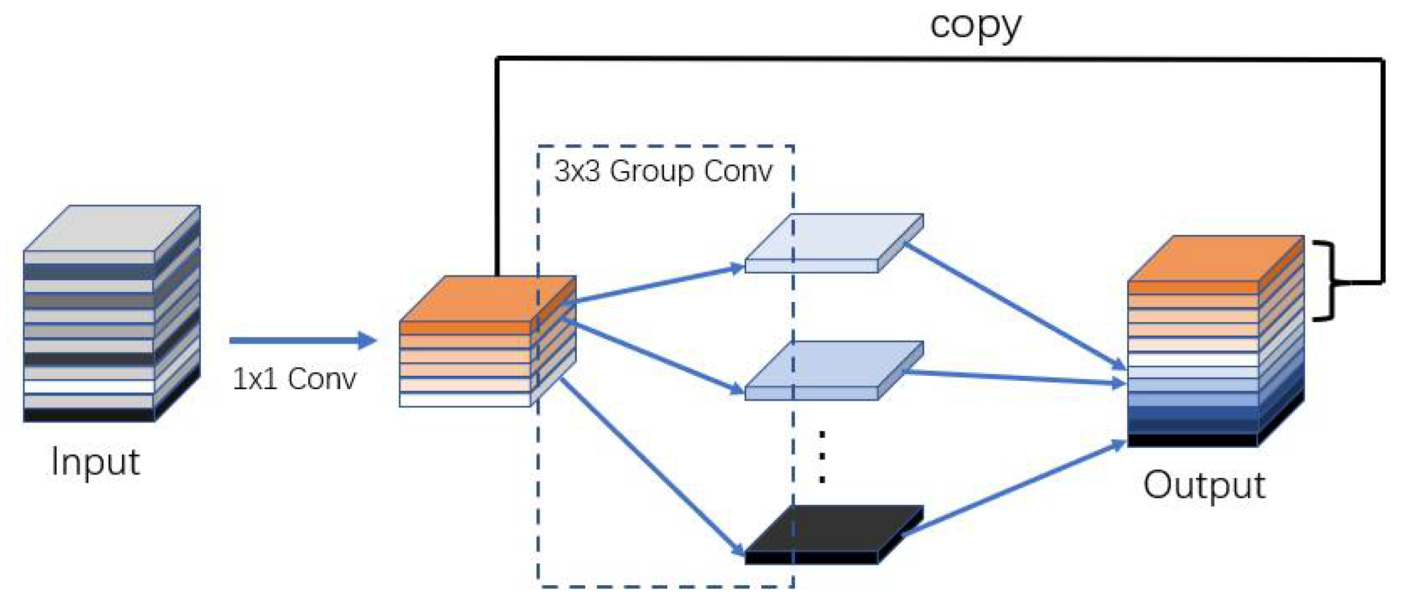
• The CSPNet structure is introduced into the original U-net structure, which can reduce the amount of computation and achieve a richer gradient combination. At the same time, except for the last layer, the Ghost module is used to replace the depth separable convolution, which further reduces the size of the image enhancement model.
• The channel consistency loss is introduced into the non-reference loss: using KL divergence to enhance the consistency between the original image and the enhanced image on the difference between channels.

Section 2 introduces the overall architecture of Zero-DCE Tiny and the non-reference loss function used. Section 3 introduces the parameter setting of the Ablation Experiment and the comparison of relevant experimental results. Finally, this work compares the new method with Zero-DCE and Zero-DCE++ methods in sensory and quantitative aspects and tests the effect of each method in the downstream application.

2. Related Works

In this section, we mainly focus on the relevant work of zero sample learning in the field of image enhancement and summarize some commonly used model lightweight methods.

2.1. Zero Sample Learning for Image Enhancement

Zhang et al. [14] proposed a zero-order learning method that uses Exposure Correction Network (ExCNet) for backlight image restoration. It first uses a depth network to estimate the S-curve. Zhu et al. [15] proposed a three-branch CNN, called RRDNet, to repair the underexposed image by decomposing the input image into illuminance, reflectivity, and noise. Several kinds of loss functions are specially designed to drive zero-order learning. Zhao et al. [16] performed Retinex decomposition through a neural network and then used the RetinexDIP model based on Retinex to enhance low illumination images. Inspired by deep image priority (DIP) [17], RetinexDIP takes randomly sampled white noise as input, generates reflection components and illumination components through Retinex decomposition, and then uses the obtained illumination components for image enhancement. The training process uses some losses as constraints, such as reflection loss. Liu et al. [18] proposed a new principled framework to search for a lightweight priority architecture for low-light-level images in real scenes by injecting knowledge of low-light-level images. Zero-DCE [5] regards light enhancement as a curve estimation task for images. It takes low-light images as input and generates high-order curves as its output. These curves are used to adjust the input dynamic range at the pixel level to obtain an enhanced image. In addition, a fast and lightweight version called Zero-DCE++ [6] is proposed. Because the mapping from image to curve only needs a lightweight network, it realizes fast estimation.

2.2. Model Lightweight Method

Howard et al. [19] proposed the MobileNet network. In this network, the depth separable convolution is used to replace the ordinary convolution for the first time. The depth separable convolution is mainly composed of the depthwise convolution and the pointwise convolution. The depthwise convolution uses convolution to check the input features and convolute them respectively according to the channel to obtain the spatial information of the features, and the pointwise convolution uses 1 × 1 to obtain the information between different channels in the feature and achieve the lightweight effect through this combination method. In the ShuffleNet [20], the feature map obtained by group convolution was randomly and uniformly scrambled in deep separable convolution on the channel, and then a group convolution operation was carried out to replace the pointwise convolution operation, which also solved the problem of the lack of information exchange between different groups in the training process, as well as maintained the feature extraction ability of the neural network while reducing the weight. Han K et al. [21] proposed the GhostNet to solve the problem of traditional convolution containing a large amount of redundant information when extracting features. First, conventional convolution is performed with fewer convolution check inputs to obtain output features with fewer channels. After linear transformation of these features, the ghost feature map is obtained, and then the final feature map is obtained by splicing with the output features. Chien Yao Wang et al. [22] proposed the CSPNet to solve the incompatibility between deep separable convolution technology and some industrial IC designs. This network not only realizes richer gradient combinations but also reduces the calculation of the model.

3. Materials and Methods

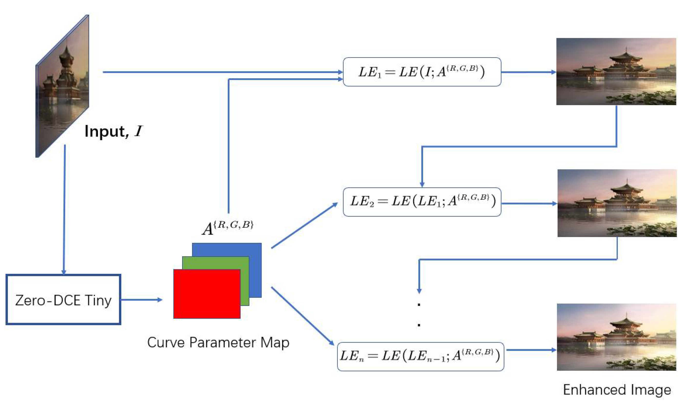
3.1. Overall Architecture

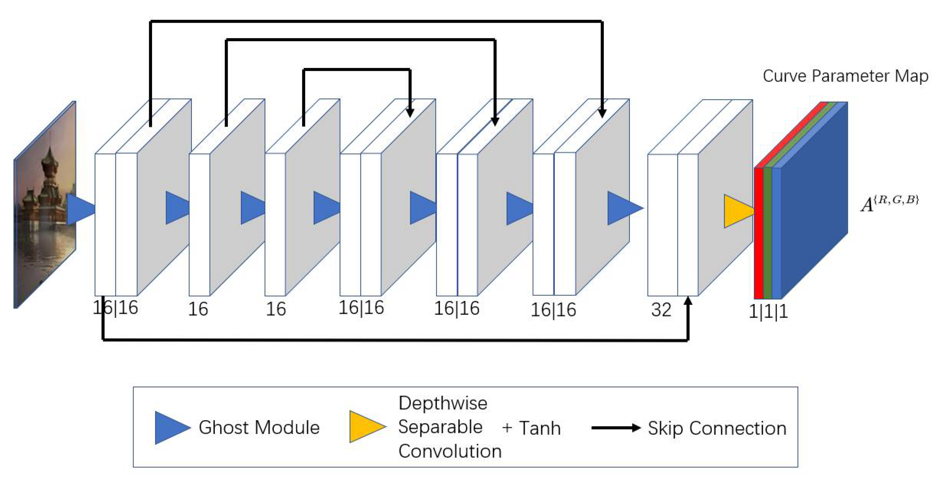
This work inherits the method of image enhancement in the Zero-DCE++ paper [6], learns the mapping curve from a weak light image to a strong light image through a convolution neural network, and then uses the learned mapping curve to iteratively adjust the pixels of the original image for many times to achieve the purpose of adjusting the image in a large dynamic range. It is assumed that the enhancement curve parameter map $A_n\left(x\right)$ obtained through network learning is related to the coordinates of pixels. A corresponding enhancement curve will be applied to each pixel on the original image. The expression of the designed image enhancement is shown in Equation (1):

$$L{E}_n\left(x\right)=L{E}_{n-1}\left(x\right)+A_n\left(x\right)L{E}_{n-1}\left(x\right)\left(1-L{E}_{n-1}\left(x\right)\right)$$

(1)

where I represents the input image and n is the number of iterations. In this work, n is set to 8, which can achieve the relatively best image enhancement results. $L{E}_n\left(x\right)$ is an enhanced version of the last enhanced image $L{E}_{n-1}\left(x\right)$, and $A_n\left(x\right)$ is a curve parameter mapping that has the same size as the given image. The process of image enhancement using Zero-DCE Tiny is shown in Figure 1.

3.2. DCE-Net Tiny

The original DCE-Net [5] used a simple CNN composed of seven convolution layers. It has a U-net structure. In the first six convolution layers, each convolution layer consists of 32 convolution layers, the kernel size is 3 × 3 of which stride is 1, followed by the ReLU activation function. The last convolution layer consists of 32 convolution layers with a size of 3 × 3 of which stride is 1, followed by the Tanh activation function, which generates 24 curve parameter mappings for eight iterations, in which each iteration generates three curve parameter mappings for three channels (i.e., RGB channels). The downsampling and batch normalization layers that destroy the relationship between adjacent pixels are discarded. Later, in Zero-DCE++ [6], the ordinary convolution processing was replaced by the deep separable convolution to reduce the amount of computation. Wherein the size of the depthwise convolution kernel is 3 × 3, the stride is 1, and when the pointwise convolution kernel size is 1 × 1, the stride is 1. At the same time, the output layer only generates 3 curve parameter maps and then reuses them in different iteration stages. This will reduce the risk of oversaturation.

The reason for choosing this U-net structure is that the U-net structure can effectively integrate multi-scale features, which are very important to achieve satisfactory low illumination enhancement. However, layer hopping connections used in U-net networks may introduce redundant feature information into the final results. Therefore, we need to design a network that effectively combines shallow features and deep features to achieve the purpose of being lightweight but effective. Inspired by CSPNet [22] and GhostNet [21], we designed the model shown in Figure 2 to replace the previous model structure.

In the new structure, the basic feature maps are split into two parts through the channel. The former is directly connected to the output layer, and the latter will act as the DCE-net [5]. With the exception of the last layer, which still uses deep separable convolution, other layers are replaced by Ghost modules. As shown in Figure 3, the Ghost module first uses 1 × 1 convolution to condense the input feature map to achieve cross-channel feature extraction. After obtaining the condensed feature, it uses a 3 × 3 convolution kernel to convolute layer-by-layer to obtain an additional feature map. Finally, it stacks the 1 × 1 convolution result and the layer-by-layer convolution result to obtain the final feature map. The feature map obtained in the two steps is processed by the ReLU activation function. In Zero-DCE Tiny, the last convolutional layer is still followed by the Tanh activation function, and the input is iterated 8 times through the curve parameter map to generate the final enhanced image.

The new network structure uses the Ghost modules to replace the depthwise separable convolution operation, which greatly improves the utilization efficiency of the feature map and reduces the amount of calculation. At the same time, introducing the CSPNet structure realizes richer feature fusion and strengthens the learning ability of the network. Moreover, the final amount of calculation is further reduced due to the segmentation of the base feature map.

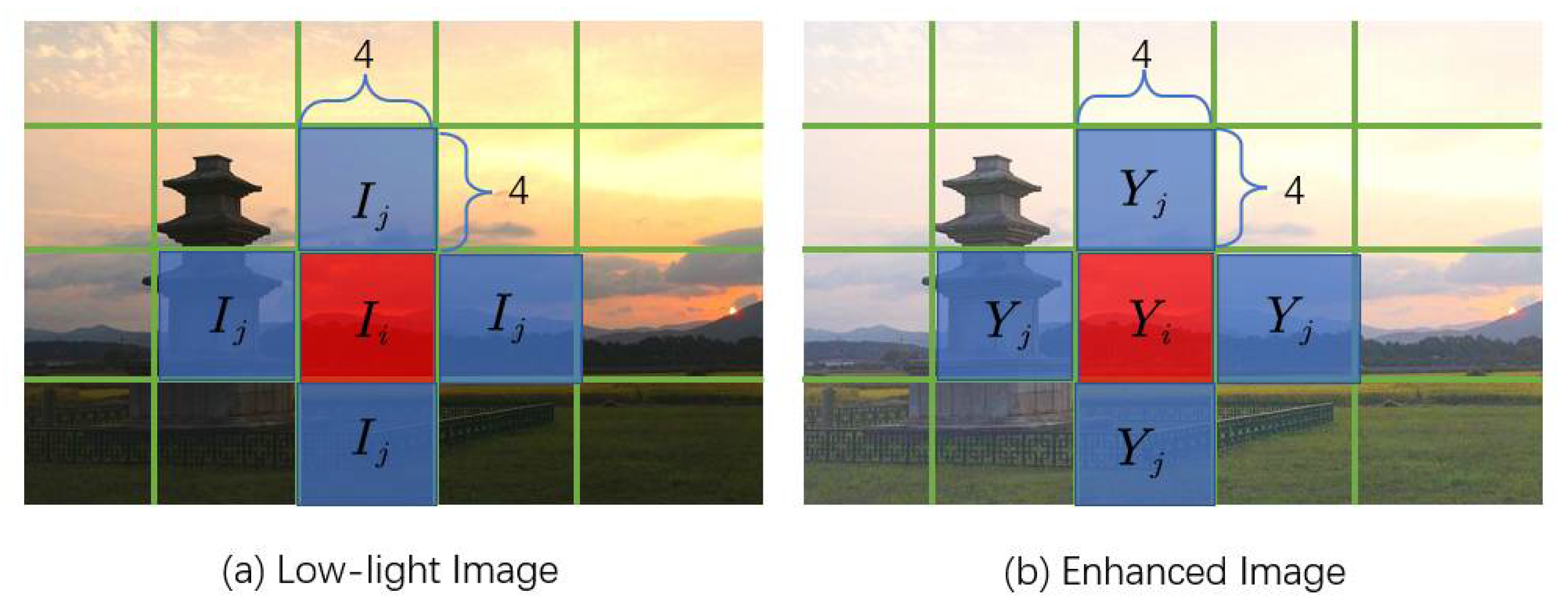
3.3. Non-Reference Loss Functions

This work inherits the non-reference loss function used in the Zero-DCE++ paper [6]. Spatial consistency loss is mainly used to maintain the difference between the adjacent areas between the input image and its enhanced version and to encourage the spatial consistency of the enhanced image.

$$L_{spa}=\frac{1}{K}\sum _{i=1}^K\sum _{j\in \Omega \left(i\right)}{\left(\left|\left(Y_i-Y_j\right)\right|-|I_i-I_j|\right)}^2$$

(2)

where K is the number of the local region and $\Omega \left(i\right)$ represents a collection of adjacent areas centered at the region i. As shown in Figure 4, Y and I are the average pixel value of the local region in the enhanced image and the original image. Our local region is set to 4 × 4.

Exposure Control Loss is used to control the exposure level. $L_{\exp }$ can be expressed as:

$$L_{\exp }=\frac{1}{M}{\sum }_{k=1}^M|Y_k-E|$$

(3)

where M is the number of nonoverlapping local regions of size 16 × 16, the average pixel value of a local region in the enhanced version is denoted as Y, and E indicates a good exposure level.

The loss of color constancy is mainly used to reduce color deviation in enhanced images, which can be expressed as:

$$L_{col}={\sum }_{\forall \left(p,q\right)\in \epsilon }{\left(J^p-J^q\right)}^2, \epsilon =\left\{\left(R,G\right),\left(R,B\right),\left(G,B\right)\right\}$$

(4)

where $J^p$ denotes the pixel average value of the p channel in the enhanced image, and (p, q) represents a pair of channels.

The loss of illumination smoothness keeps the adjacent pixel values monotonous, thus avoiding overexposure and underexposure, which can be expressed as:

$$L_{t{v}_A}=\frac{1}{N}\underset{n=1}{\sum ^N}\sum _{c\in \xi }{\left(\left|{\nabla }_x{A}_n^c\right|+\left|{\nabla }_y{A}_n^c\right|\right)}^2,\xi =\left\{R,G,B\right\}$$

(5)

where N is the number of iterations, and ${\nabla }_x$ and ${\nabla }_y$ represent the horizontal and vertical gradient operations, respectively.

Inspired by the spatial consistency loss, this work proposes a new non-reference loss: channel consistency loss. As a new loss, channel consistency loss mainly enhances the consistency between the original image and the enhanced image in the channel pixel difference through KL divergence, and suppresses the generation of noise information and invalid features to improve the image enhancement effect. The channel consistency loss can be expressed as:

$$L_{kl}=KL\left[R-B\left|\right|R^{\prime }-B^{\prime }\right]+KL\left[R-G\left|\right|R^{\prime }-G^{\prime }\right]+KL\left[G-B\left|\right|G^{\prime }-B^{\prime }\right]$$

(6)

In this work, R, G, and B represent the color channels of the original image, $R^{\prime }$, $G^{\prime }$ and $B^{\prime }$ represent the three-color channels of the enhanced image, and KL divergence is used to represent the difference between the two distributions. If the difference between the two is small, the KL divergence is small. When the two distributions are consistent, the KL divergence value is 0.

The total loss can be expressed as:

$$L_{total}=W_{spa}{L}_{spa}+W_{\exp }{L}_{\exp }+W_{col}{L}_{col}+W_{t{v}_A}{L}_{t{v}_A}+W_{kl}{L}_{kl}$$

(7)

where $W_{spa}$, $W_{\exp }$, $W_{col}$, and $W_{kl}$ are the weights of the losses.

4. Results

To be consistent with the previous work [5,6], we also used 360 multiple exposure sequences from Part 1 of the SICE dataset [23] as our training dataset. We randomly divided 3022 images with different exposure levels in the Part 1 [23] subset into two parts (2422 images for training and 600 images for validation). The images were resized to 512 × 512 × 3. We implemented our framework on RTX3060 GPU using PyTorch. The batch size is 8. We used a Gaussian function with a mean of 0 and a standard deviation of 0.02 to initialize the convolutional neural network and used the Adam optimizer to optimize the network. The Adam optimizer uses default parameters and a constant learning rate. The weights $W_{spa}$, $W_{\exp }$, $W_{col}$, and $W_{kl}$ were set to 1, 10, 5, 1600, and 5 to balance the loss ratio. Network training 100 rounds in total.

We used some public datasets for testing, including LIME [24] (10 images), and DICM [25] (64 images). In addition, we also collected a total of 2300 low light/normal light images on the part2 subset of the SICE dataset as the test dataset, and all images were adjusted to 1200 × 900 × 3.

4.1. Ablation Study

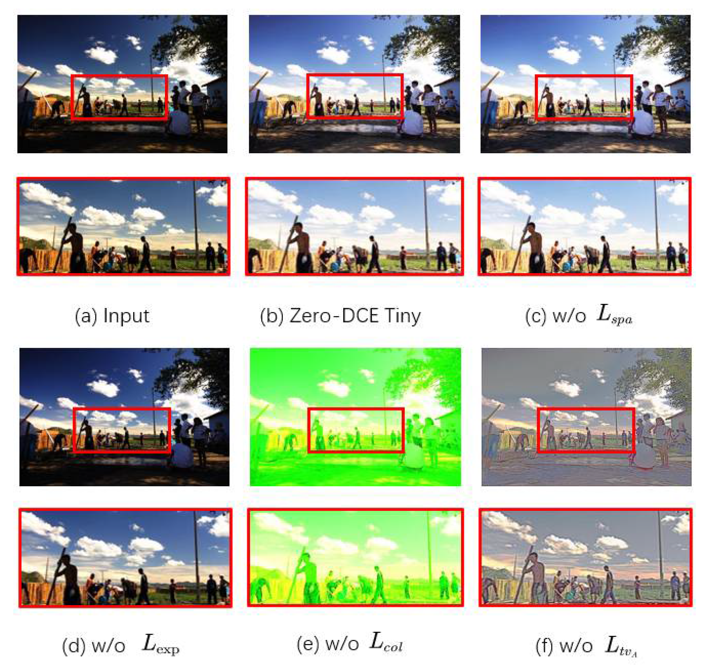
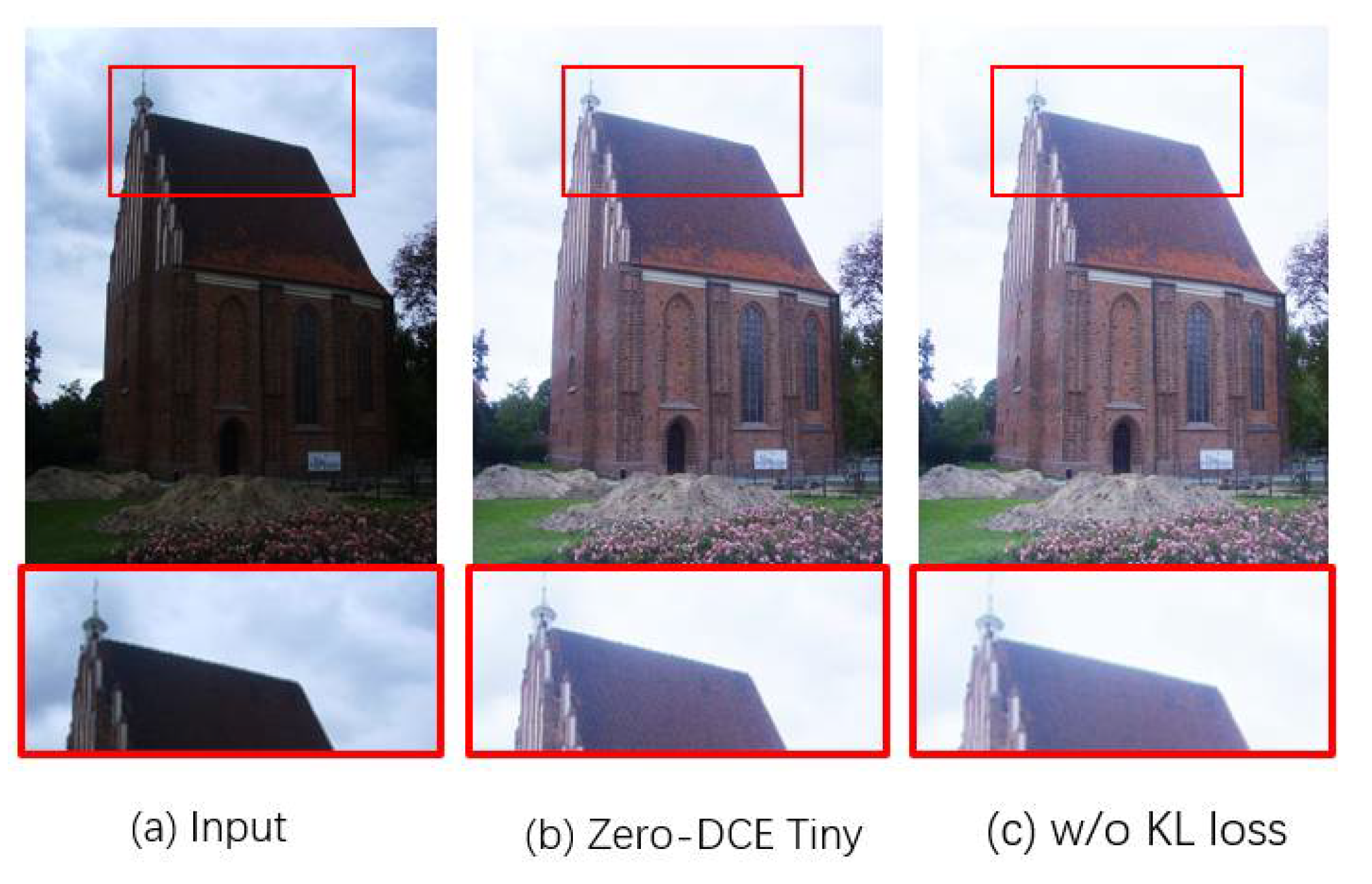
4.1.1. Ablation Study of Each Loss

We performed ablation experiments on each loss function; the results are shown in Figure 5. As shown in Figure 5c, lack of spatial consistency loss $L_{spa}$ reduces the image contrast, for example, the part of the cloud in the image. As shown in Figure 5d, lack of exposure control loss $L_{\exp }$ causes image enhancement invalid. As shown in Figure 5e, When the loss of color constancy $L_{col}$ is discarded, serious color projection occurs. Finally, as shown in Figure 5f, removing the light smoothness loss $L_{t{v}_A}$ leads to obvious artifacts.

We added the channel consistency loss to the original version of the non-reference loss function and performed ablation experiments. Figure 6 compares the sensory results of the test image: After adding the loss of spatial consistency, the enhanced image is more natural and the overall contrast distribution of the image is more balanced. As shown in Figure 6, the house is less affected by the halo, and the details are clearer.

4.1.2. Ablation Study of Backbone Network

For the new backbone network, we introduce the CSPNet network structure and set the number of feature maps in the base layer to 32. We divide the basic feature maps into two parts. The former is directly connected to the output layer, and the latter will act as the DCE-net [5]. At the same time, we replace all depth separable convolutions outside the last layer with the Ghost module.

Table 1. Parameter comparison of the backbone network; the parameter is computed for an image of size 256 × 256 × 3.

Method	Total Params	Total Memory	Total Flops	Total MAdd	Total MemR + W
Zero-DCE	79,416	62.00 MB	10.38 GFlops	5.21 GMAdd	143.05 MB
Zero-DCE++	10,561	129.50 MB	1.32 GFlops	694.22 MMAdd	283.04 MB
Only CSPNet structure	5153	93.50 MB	632.68 MFlops	339.8 MMAdd	199.02 MB
only Ghost module	5331	112.75 MB	689.96 MFlops	361.96 MMAdd	273.52 MB
Zero-DCE Tiny	2731	104.75 MB	353.37 MFlops	190.51 MMAdd	215.51 MB

shows the original network and three network parameters. We divide the network structure into three types: “Only CSPNet structure”, “Only Ghost module”, and “Zero-DCE Tiny”. We mainly compare five parameters, namely the number of network parameters (Total params), the amount of memory required for node reasoning (Total memory), the number of floating-point operations (Total Flops), the amount of multiplication and addition required for network reasoning (Total Madd), and the sum of memory read and write (Total MemR + W). It can be seen from Table 1 that Zero-DCE Tiny has achieved a lighter effect on multiple indicators. However, since the Ghost module uses a large number of group convolutions, resulting in more memory occupancy, the “Total Madd” and “Total MemR + W” metrics are slightly higher than “Only CSPNet structure”. However, the experiments show that “Only CSPNet structure” will lead to a poor image enhancement effect, so we finally choose to obtain better image enhancement performance at the cost of certain memory occupation.

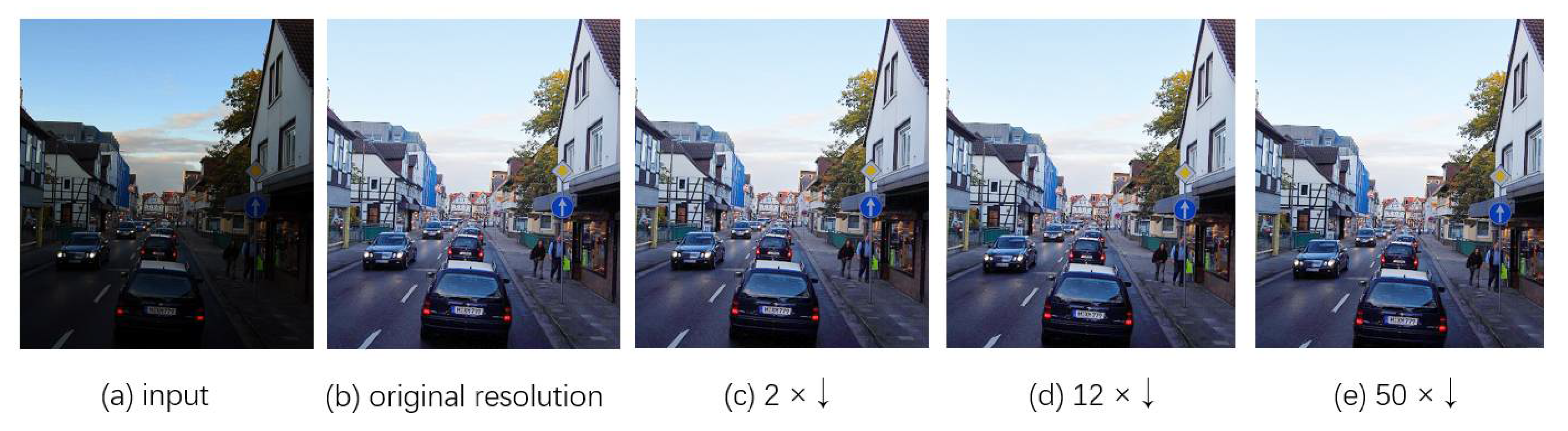
4.1.3. Ablation Study of Input Size

We provide input of different sizes for Zero-DCE Tiny.

Table 2. Effect of different input image resolutions on image enhancement. The FLOPs (in G) are computed for an image of size 1200 × 900 × 3. “number × ↓” indicates the times of downsampling the input image. The test image is from the part2 dataset of SCIE.

Metrics	Original Resolution	2 × ↓	4 × ↓	6 × ↓	12 × ↓	20 × ↓	50 × ↓
PSNR	16.14	16.22	16.38	16.45	16.42	15.95	15.02
FLOPs	5.82	1.46	0.355	0.158	0.039	0.014	0.002

summarizes the statistical relationship between enhanced performance and input size. We also show some results by modifying the size of the network input image, as shown in Figure 7. As shown in Figure 7 and Table 2, the downsampling input size has no significant impact on the enhanced performance, but significantly saves computing costs. As shown in Table 2, 6 × ↓ obtained the highest average PSNR value, but because 12 × ↓ is better in model efficiency, we use it as the default configuration for the new network.

4.2. Benchmark Evaluations

In this section, we compare the new method with the classical benchmark models in qualitative and quantitative experiments. Finally, the new image enhancement method’s gain effect on object detection in the dark is tested.

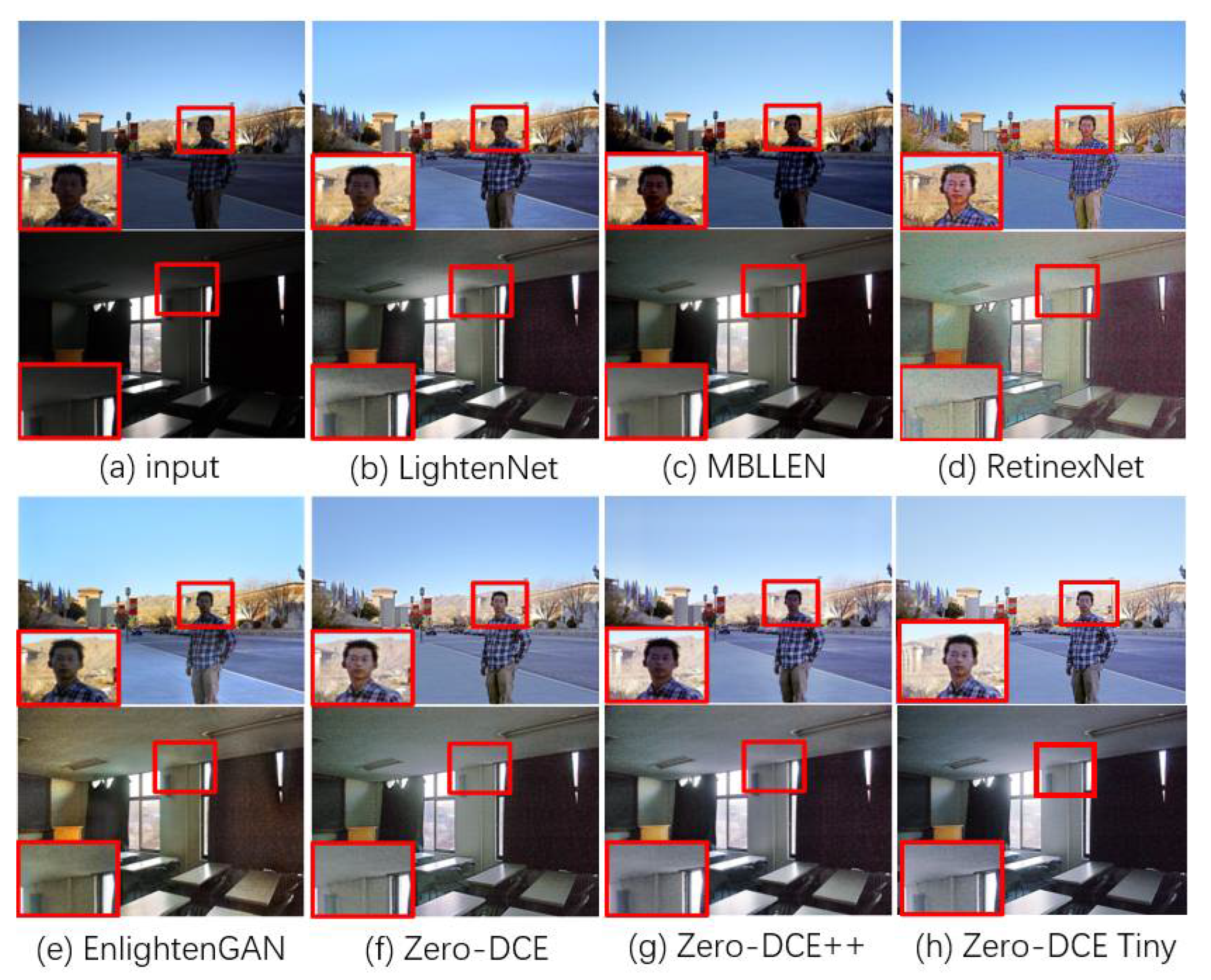
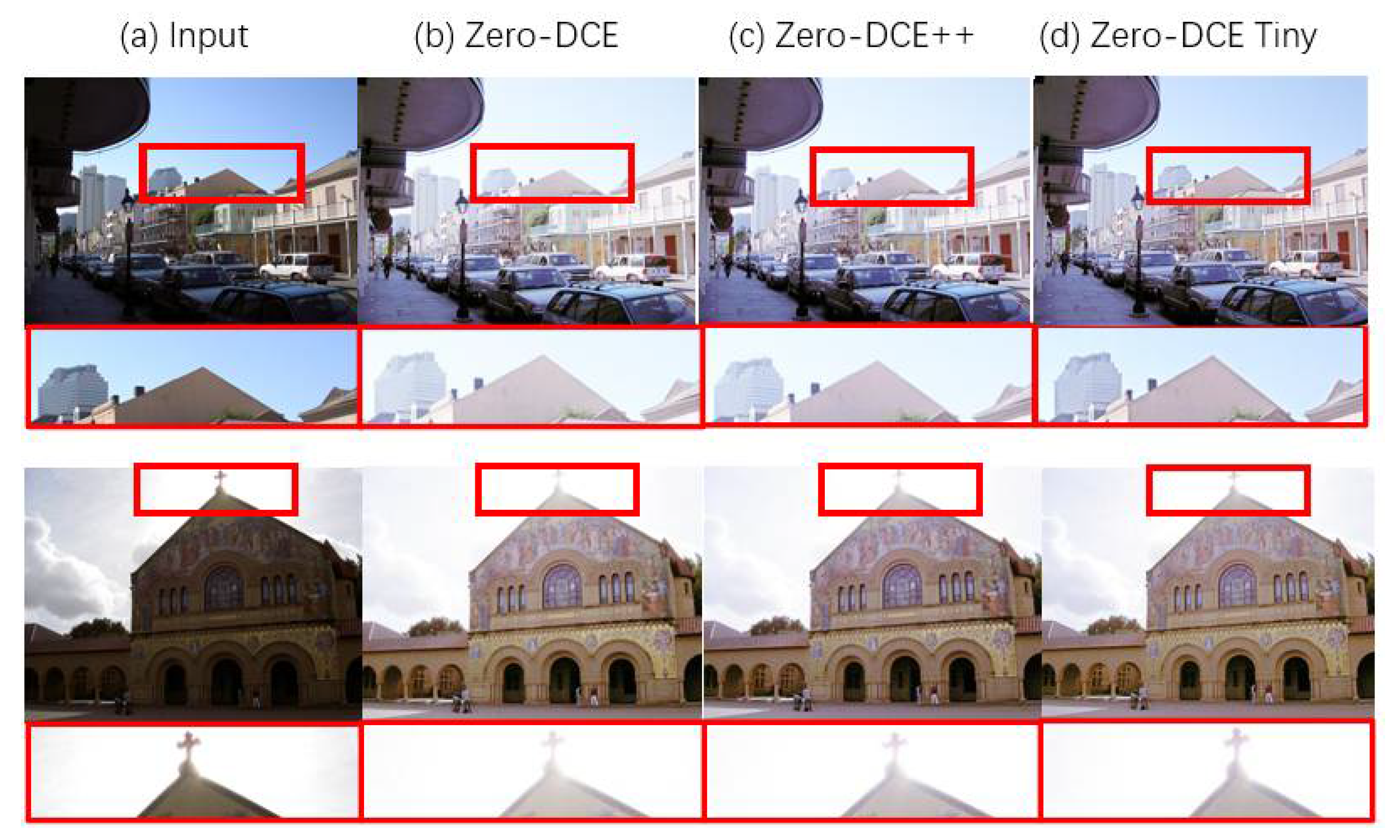
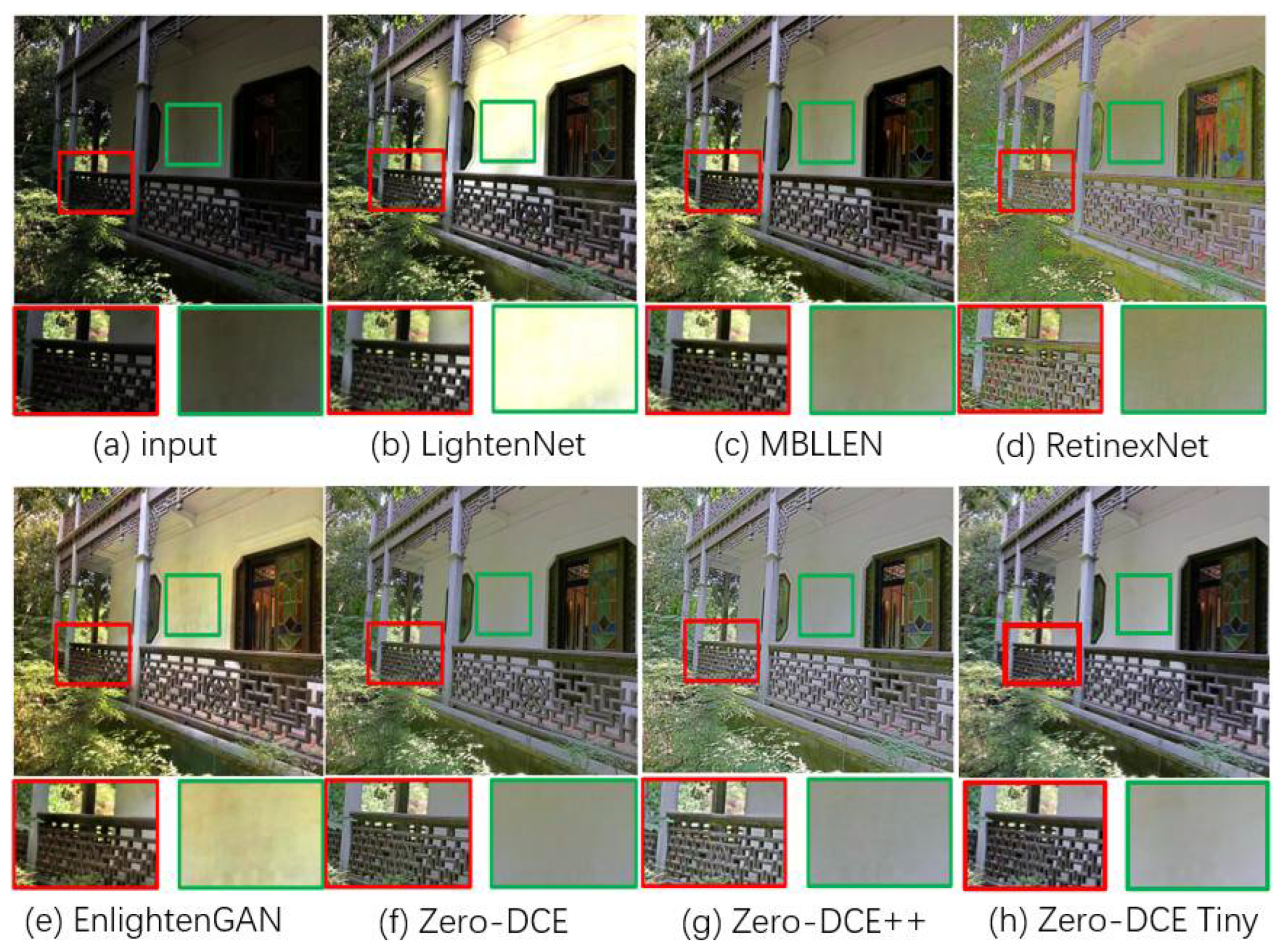
4.2.1. Visual and Perceptual Comparisons

We selected some classical benchmark methods to compare them with our methods for visual and perceptual comparisons. The new method chooses Zero-DCE Tiny as the backbone network, and adds the spatial consistency loss to the non-reference loss for training and testing. Figure 8 shows the enhanced image effects of some test images obtained by different methods under the same conditions. We tested three CNN-based methods (RetinexNet [9], LightenNet [26], MBLLEN [8]) and one GAN-based method (EnlightenGAN [27]) to replicate the results using open-source code.

Figure 8 shows the results of our tests on the SICE dataset. For outdoor scenes, the LightenNet, the MBLLEN, and the EnlightenGAN find it difficult to achieve clear enhancement results for difficult backlight areas, such as the face part. For RetinexNet, there are many overexposure cases in the image, including the face part, with poor overall sensory effects. For indoor scenes, MBLLEN performs well visually, but it is too smooth, which may filter out the detailed features of the original image. For RetinexNet, the noise information in the image is amplified, resulting in a poor enhancement effect. For EnlightenGAN, the enhanced image shows a certain color deviation. For the Zero-DCE series methods, the effects of Zero-DCE and Zero-DCE tiny methods are very close. Compared with Zero-DCE++, the enhancement effect of the face region is better.

In the experiment, we found that in the Zero-DCE series of methods, the image enhancement effect of Zero-DCE Tiny is softer, as shown in Figure 9. For areas with strong sunlight, the roof part and the cross part in the enhanced image of Zero-DCE Tiny are clearer. At the sensory level, it shows that the new method is conducive to suppressing the problem of excessive local exposure.

The part2 subset of SCIE dataset is also used to compare different methods. The comparison results are shown in Figure 10. The LightenNet has obvious light spots in the wall area, and RetinexNet, EnlightenGAN, and Zero-DCE++ all have different degrees of color deviation. The image enhancement results of MBLLEN are dark, whereas the results of Zero-DCE and Zero-DCE Tiny are very close. The image enhancement result obtained by Zero-DCE Tiny is closer to the natural situation in color and contrast, and the sensory effect is better.

4.2.2. Quantitative Comparisons

Table 3. Comparison of image enhancement indexes.

Metrics	PSNR	SSIM	MAE
MBLLEN	15.02	0.52	119.14
RetinexNet	15.99	0.53	104.81
LightenNet	13.17	0.55	140.92
EnlighenGAN	16.21	0.59	102.78
Zero-DCE	16.57	0.59	98.78
Zero-DCE++	16.42	0.58	102.87
Zero-DCE Tiny	16.50	0.61	102.52

shows the quantitative comparison of several image enhancement methods. We compared three image enhancement indicators on the part2 test dataset [23]: peak signal to noise ratio (PSNR), structural similarity (SSIM), and mean absolute error (MAE), where the SSIM value represents the similarity between the results and the real results in terms of structural characteristics. The PSNR value (in the case of a low MAE value) indicates that the results obtained are closer to the actual situation.

It can be seen from Table 3 that by introducing a new backbone network and channel consistency loss, the PSNR index and SSIM index are improved compared with Zero-DCE++ (when the MAE value is low), wherein the SSIM index even exceeds Zero-DCE. It shows that the loss of channel consistency helps improve the structural consistency of the original image and the enhanced image. At the same time, from Table 1 and

Table 4. Model running speed comparison.

Metrics	Runtime (s)	Total Params	Platform
MBLLEN	13.9949	450,171	TensorFlow (GPU)
RetinexNet	0.1200	555,205	TensorFlow (GPU)
LightenNet	25.7716	29,532	MATLAB (CPU)
EnlighenGAN	0.0078	8,636,675	PyTorch (GPU)
Zero-DCE	0.0025	79,416	PyTorch (GPU)
Zero-DCE++	0.0012	10,561	PyTorch (GPU)
Zero-DCE Tiny	0.0008	2731	PyTorch (GPU)

, we know that compared with Zero-DCE++, our network is more lightweight and the reasoning speed is more friendly to practical applications. At the same time, due to the reduction of the number of parameters, during our training, it only takes 35 min to train the model with a single RTX3060 graphics card. So, it is also very friendly to the second training of developers. In general, the new model is a more efficient image enhancement model that achieves lightweight while maintaining a good image enhancement effect.

4.2.3. Object Detection in the Dark

To test the gain effect of the improved image enhancement algorithm in the downstream application, we selected the object detection task in the low light environment to test the new algorithm. We mainly tested on the ExDark dataset [28], which was built specifically for low-light-level image recognition tasks. The ExDark dataset consists of 7363 low-light images which are marked as 12 object classes. We only use its test dataset, take Zero-DCE Tiny as the preprocessing step, and then use the pretrain ResNet50 classifier through the ImageNet. In the weak light test set, Zero-DCE Tiny was used as pretreatment to improve the classification accuracy from 22.02% (top-1) and 39.46% (top-5) to 27.86% (top-1) and 44.86% (top-5) after enhancement. This provides side evidence that image enhancement using Zero-DCE Tiny not only produces pleasant visual effects but also provides richer image details for downstream applications, which is conducive to improving the application effect of downstream applications.

5. Discussion

The new model Zero-DCE Tiny proposed in this paper is a further lightweight product of the Zero-DCE series models. The comprehensive results of multiple test datasets show that the new model can deal with low-light images in various scenarios well. In Furthermore, compared with the Zero-DCE++ version, the efficiency of the model is further improved. Shorter reasoning time and lower training cost make the new model more friendly to practical applications; this will promote the application of the deep learning image enhancement model in real life, such as the night vision instrument. More importantly, the upstream benefits of image enhancement will benefit downstream applications, so that image processing algorithms such as image detection and semantic segmentation can better cope with images in complex environments.

6. Conclusions

We propose a new backbone network Zero-DCE Tiny to replace Zero-DCE++ for low illumination image enhancement. It can use zero reference images for end-to-end training. At the same time, compared with the original method, the backbone network used in this paper not only enhances the feature fusion but also reduces the amount of computation and memory consumption. This paper also tests the new non-reference loss to verify the effectiveness of channel consistency loss in improving image contrast balance. The results show that the new image enhancement method can better balance the image enhancement effect and the lightweight level of the model. This will further promote the application of the deep learning model in the field of image enhancement. However, the method proposed in this work also has some problems to be solved. For example, although this image enhancement model enhances the fusion of features, it inevitably introduces noise and redundant information. Therefore, there is still much room for improvement in the effect of image enhancement. In the future, we will try more noise suppression methods to retain the semantic information in the original image and enhance the promotion of image enhancement to downstream applications.

References

1. Iqbal, M.S.; Ahmad, I.; Bin, L.; Khan, S.; Rodrigues, J.J.P.C. Deep learning recognition of diseased and normal cell representation. Trans. Emerg. Telecommun. Technol. 2020, 32, e4017. [Google Scholar] [CrossRef]
2. Ainetter, S.; Fraundorfer, F. End-to-end Trainable Deep Neural Network for Robotic Grasp Detection and Semantic Segmentation from RGB. In Proceedings of the 2021 IEEE International Conference on Robotics and Automation (ICRA), Xi’an, China, 30 May–5 June 2021. [Google Scholar]
3. Abdullah-Al-Wadud, M.; Kabir, H.; Dewan, M.A.A.; Chae, O. A Dynamic Histogram Equalization for Image Contrast Enhancement. Int. Conf. Consum. Electron. 2007, 53, 593–600. [Google Scholar] [CrossRef]
4. Wang, S.; Zheng, J.; Hu, H.; Li, B. Naturalness Preserved Enhancement Algorithm for Non-Uniform Illumination Images. IEEE Trans. Image Process. 2013, 22, 3538–3548. [Google Scholar] [CrossRef] [PubMed]
5. Guo, C.; Li, C.; Guo, J.; Loy, C.C.; Hou, J.; Kwong, S.; Cong, R. Zero-Reference Deep Curve Estimation for Low-Light Image Enhancement. In Proceedings of the IEEE/CVF Conference on Computer Vision and Pattern Recognition (CVPR), Seattle, WA, USA, 14–19 June 2020. [Google Scholar]
6. Li, C.; Guo, C.; Loy, C.C. Learning to Enhance Low-Light Image via Zero-Reference Deep Curve Estimation. arXiv 2021, arXiv:2103.00860. [Google Scholar] [CrossRef] [PubMed]
7. Lore, K.G.; Akintayo, A.; Sarkar, S. LLNet: A Deep Autoencoder Approach to Natural Low-light Image Enhancement. Pattern Recognit. 2015, 61, 650–662. [Google Scholar] [CrossRef]
8. Lv, F.; Lu, F.; Wu, J.; Lim, C. MBLLEN: Low-Light Image/Video Enhancement Using CNNs. Br. Mach. Vis. Conf. 2018, 220, 4. [Google Scholar]
9. Wei, C.; Wang, W.; Yang, W.; Liu, J. Deep Retinex Decomposition for Low-Light Enhancement. arXiv 2018, arXiv:1808.04560. [Google Scholar]
10. Zhang, Y.; Zhang, J.; Guo, X. Kindling the Darkness: A Practical Low-light Image Enhancer. In Proceedings of the 27th ACM International Conference on Multimedia, Nice, France, 21–25 October 2019. [Google Scholar]
11. Ren, W.; Liu, S.; Ma, L.; Xu, Q.; Xu, X.; Cao, X.; Du, J.; Yang, M. Low-Light Image Enhancement via a Deep Hybrid Network. IEEE Trans. Image Process. 2019, 28, 4364–4375. [Google Scholar] [CrossRef] [PubMed]
12. Lim, S.; Kim, W.J. DSLR: Deep Stacked Laplacian Restorer for Low-Light Image Enhancement. IEEE Trans. Multimed. 2021, 23, 4272–4284. [Google Scholar] [CrossRef]
13. Zhang, Y.; Guo, X.; Ma, J.; Liu, W.; Zhang, J. Beyond Brightening Low-light Images. Int. J. Comput. Vis. 2021, 129, 1013–1037. [Google Scholar] [CrossRef]
14. Zhang, L.; Zhang, L.; Liu, X.; Shen, Y.; Zhang, S.; Zhao, S. Zero-Shot Restoration of Back-lit Images Using Deep Internal Learning. In Proceedings of the 27th ACM International Conference on Multimedia, Nice, France, 21–25 October 2019. [Google Scholar]
15. Zhu, A.; Zhang, L.; Shen, Y.; Ma, Y.; Zhao, S.; Zhou, Y. Zero-Shot Restoration of Underexposed Images via Robust Retinex Decomposition. In Proceedings of the 2020 IEEE International Conference on Multimedia and Expo (ICME), London, UK, 6–10 July 2020. [Google Scholar]
16. Zhao, Z.; Xiong, B.; Wang, L.; Ou, Q.; Yu, L.; Kuang, F. RetinexDIP: A Unified Deep Framework for Low-light Image Enhancement. IEEE Trans. Circuits Syst. Video Technol. 2021, 32, 1076–1088. [Google Scholar] [CrossRef]
17. Ulyanov, D.; Vedaldi, A.; Lempitsky, V. Deep Image Prior. Int. J. Comput. Vis. 2017, 128, 1867–1888. [Google Scholar] [CrossRef]
18. Liu, R.; Ma, L.; Zhang, J.; Fan, X.; Luo, Z. Retinex-inspired Unrolling with Cooperative Prior Architecture Search for Low-light Image Enhancement. In Proceedings of the IEEE/CVF Conference on Computer Vision and Pattern Recognition (CVPR), Nashville, TN, USA, 20–25 June 2021. [Google Scholar]
19. Howard, A.; Zhu, M.; Chen, B.; Kalenichenko, D.; Wang, W.; Weyand, T.; Andreetto, M.; Adam, H. MobileNets: Efficient Convolutional Neural Networks for Mobile Vision Applications. Computer Vision and Pattern Recognition. arXiv 2017, arXiv:1704.04861. [Google Scholar]
20. Zhang, X.; Zhou, X.; Lin, M.; Sun, J. ShuffleNet: An Extremely Efficient Convolutional Neural Network for Mobile Devices. In Proceedings of the IEEE Conference on Computer Vision and Pattern Recognition (CVPR), Salt Lake City, UT, USA, 18–23 June 2018. [Google Scholar]
21. Han, K.; Wang, Y.; Tian, Q.; Guo, J.; Xu, C.; Xu, C. GhostNet: More Features from Cheap Operations. In Proceedings of the IEEE/CVF Conference on Computer Vision and Pattern Recognition (CVPR), Long Beach, CA, USA, 15–20 June 2019. [Google Scholar]
22. Wang, C.; Liao, H.M.; Yeh, I.-H.; Wu, Y.; Chen, P.; Hsieh, J. CSPNet: A New Backbone that can Enhance Learning Capability of CNN. In Proceedings of the IEEE/CVF Conference on Computer Vision and Pattern Recognition (CVPR) Workshops, Long Beach, CA, USA, 15–20 June 2019. [Google Scholar]
23. Cai, J.; Gu, S.; Zhang, L. Learning a Deep Single Image Contrast Enhancer from Multi-Exposure Images. IEEE Trans. Image Process. 2018, 27, 2049–2062. [Google Scholar] [CrossRef] [PubMed]
24. Guo, X.; Li, Y.; Ling, H. LIME: Low-light image enhancement via illumination map estimation. IEEE Trans. Image Process. 2017, 26, 982–993. [Google Scholar] [CrossRef] [PubMed]
25. Lee, C.; Lee, C.; Kim, C.-S. Contrast enhancement based on layered difference representation. IEEE Trans. Image Process. 2012, 22, 965–968. [Google Scholar]
26. Li, C.; Guo, J.; Porikli, F.; Pang, Y. LightenNet: A convolutional neural network for weakly illuminated image enhancement. Pattern Recognit. Lett. 2018, 104, 15–22. [Google Scholar] [CrossRef]
27. Jiang, Y.; Gong, X.; Liu, D.; Cheng, Y.; Fang, C.; Shen, X.; Yang, J.; Zhou, P.; Wang, A.Z. EnlightenGAN: Deep light enhancement without paired supervision. arXiv 2019, arXiv:1906.06972. [Google Scholar] [CrossRef] [PubMed]
28. Loh, Y.P.; Chan, C.S. Getting to Know Low-light Images with The Exclusively Dark Dataset. Comput. Vis. Image Underst. 2018, 178, 30–42. [Google Scholar] [CrossRef] [Green Version]
Figure 1. Overall structure diagram.
Electronics 11 02750 g001
Figure 2. Zero-DCE Tiny structure diagram.
Electronics 11 02750 g002
Figure 3. Ghost module sketch map.
Electronics 11 02750 g003
Figure 4. Mapping of spatial consistency loss. Subfigure (a,b) respectively show the setting of local regions in the original image and the enhanced image.
Electronics 11 02750 g004
Figure 5. Ablation study of each loss. Subfigure (a) shows the original input, subfigure (b) shows the enhanced image result through Zero-DCE Tiny method, subfigure (cf) respectively show the image enhancement results after removing spatial consistency loss, exposure control loss, color consistency loss and illumination smoothness loss.
Electronics 11 02750 g005
Figure 6. Sensory comparison of kl loss ablation experiment. Subfigure (a) shows the original input, subfigure (b) shows the enhanced image result through Zero-DCE Tiny method, subfigure (c) shows the image enhancement result after removing channel consistency loss.
Electronics 11 02750 g006
Figure 7. Ablation study of input image size. Subfigure (a) shows the original input, subfigure (b) shows the enhanced image result when the image resolution is not changed, subfigure (ce) show the image enhancement results after downsampling the input image.
Electronics 11 02750 g007
Figure 8. A visual comparison among the results generated by different methods. Subfigure (a) shows the original input, subfigure (bh) respectively show the enhanced image results through LightenNet [26], MBLLEN [8], RetinexNet [9], EnlightenGAN [27], Zero-DCE [5], Zero-DCE++ [6] and Zero-DCE Tiny methods.
Electronics 11 02750 g008
Figure 9. Visual comparisons among the results generated by the Zero-DCE series of methods. Subfigure (a) shows the original input, subfigure (bd) respectively shows the enhanced image results through Zero-DCE [5], Zero-DCE++ [6] and Zero-DCE Tiny methods.
Electronics 11 02750 g009
Figure 10. Visual comparison of Part 2 subset of SCIE dataset. Subfigure (a) shows the original input, subfigure (bh) respectively show the enhanced image results through LightenNet [26], MBLLEN [8], RetinexNet [9], EnlightenGAN [27], Zero-DCE [5], Zero-DCE++ [6] and Zero-DCE Tiny methods.
Electronics 11 02750 g010