Railway Obstacle Intrusion Detection Based on Convolution Neural Network Multitask Learning

Abstract

The detection of train obstacle intrusion is very important for the safe running of trains. In this paper, we design a multitask intrusion detection model to warn of the intrusion of detected target obstacles in railway scenes. In addition, we design a multiobjective optimization algorithm that performs with different task complexity. Through the shared structure reparameterized backbone network, our multitask learning model utilizes resources effectively. Our work achieves competitive results on both object detection and line detection, and achieves excellent inference time performance (50 FPS). Our work is the first to introduce a multitask approach to realize the assisted-driving function in a railway scene.

1. Introduction

Due to the sudden appearance of various obstacles under the influence of various weather conditions, emergency braking must be performed when a train needs to stop in an emergency. However, considering that the weight of a train ranges from several thousand to more than ten thousand tons, its inertia during operation is very large. Therefore, once the emergency brake is applied, there must be a large forward impact force, and the people and objects in the carriage inevitably lose their balance, which leads to possible collapses and crushes, and even severe injuries. At the same time, given the extensive geographical coverage and ever-increasing total length of the railway system, staff cannot monitor all sections of the railway in real time. The distance that the human eye can recognize is limited, and telephoto lenses are used to observe the distance that the human eye cannot observe, identify obstacles in the distance, and give early warning. It is necessary to install detection equipment that assists the driver to determine whether there are obstacles in the track area, so as to determine whether the front of the train is safe. Ma [1] and Ding [2] used detection methods based on YOLOv3 [3] and YOLOv5 [4], respectively, to identify all obstacles in the current railway scene. Liu [5] added an attention module based on YOLOv4 [6] for obstacle detection in a railway scene. However, the method of object detection alone has great limitations. Obstacles in the safe area by the rails are also detected. Although they pose no threat to the safe running of the train, the detection system will still alarm and distract the attention of the staff. Considering the defect mentioned above, adding a track recognition system to judge whether the identified obstacle can pose security threats can effectively improve the accuracy and recognition rate.

For these two tasks, Wang [7] divided all railway areas for obstacle intrusion judgment. Chen [8] adopted target detection and semantic segmentation, respectively, and combined the results of the two tasks at the output level. However, when an obstacle blocked the track line, the segmentation method was not able to extract the complete information about the track line, so that the network needed to extract boundary information from the segmentation results in the postprocessing stage, and at the same time impute the missing parts, which required huge extra computing resources. Therefore, a multitask method was adopted to combine target obstacle detection and track line recognition, which directly extracted the position of the track line and reduced the waste of computing resources.

In the existing multitask-based automatic driving methods [9,10,11], because the automatic driving of the car is fully automatic and requires no human intervention, the goal focuses on improving the recall rate. However, the obstacle detection for a railway system is more inclined to assist the driver to detect long-distance obstacles in the shortest time span and to give early warning to obstacles that may have intrusion behaviors. Using the existing automatic driving methods is prone to generate a large number of false alarms and interfere with the driver which tends to cause safety issues.

Obstacle detection based on a railway scene also faces two difficulties. The first is the long braking distance. Since the speed of the train is higher than that of an ordinary vehicle in daily urban scenarios, and given the huge size of the train, emergency braking for a train requires a longer braking distance. Therefore, obstacle detection focuses more on the detection of long-distance obstacles. Another problem is the small pixel ratio of rails. Track line detection only focuses on the rails in the current track area of the train, and considering the slender shape of the rails, the target to be detected occupies very few pixels in the scene. The method of performing small target segmentation not only can hardly segment the established target, but also wastes computing resources, which does not fit the requirement of real-time detection.

Based on the above-mentioned problems, we propose a multitask intrusion detection algorithm. The network adopts a multitask design, which can simultaneously perform target obstacle detection as well as predict the location of the rail even when the track line is occluded. The network can also expand the limit area for the detected track line.

Table 1. The comparison of multitask methods in driving scenarios.

Method	Tasks	Comparison
MultiNet [9]	Classification, detection, segmentation	The classification is only used as an aid for detection and segmentation. Only detects vehicles.
YOLOP [10]	Detection, drivable area segmentation, lane line segmentation	The recall rate is high. Cannot deal with the problem of occluded lane lines.
HybridNets [11]	Detection, drivable area segmentation, lane line segmentation	Similar to YOLOP. Improves the recall rate of detection results.
Ours	Detection, track line classification, track line segmentation	Pays more attention to precision rather than recall. Segmentation assists classification results. Can effectively deal with the problem of track line being blocked

shows the comparison between the proposed method and other multitask methods in driving scenarios. When the camera detects an intrusion within the visible range, it can quickly and effectively detect the type of obstacle, determine whether the obstacle has invaded the boundary area, and give the driver different levels of warning according to the degree of intrusion. Based on this method, early warning can be done to assist the staff to drive the train safely. The contribution of this work can be summarized in three parts:

• We design a multitask intrusion detection model. The network uses the method of hard parameter sharing and shares the same encoder, which can perform the above-mentioned two different tasks to save computational cost, reduce inference time, and improve the performance of each task;
• In order to improve the speed of network operation, we adopt the track line detection method based on row classification. Using global features to predict the track line positions, it has a larger receptive field than the segmentation formula and can solve the occlusion problem;
• Based on the proposed multitask network, we propose a multiobjective optimization method that utilizes the complexity of different tasks to optimize the results.

The rest of this paper is structured as follows. Section 2 gives a brief overview of obstacle detection, lane line detection, and multitasking network framework. Section 3 details our proposed algorithm. Section 4 introduces the dataset used in this paper, presents the training results, and performs the inference process. Section 5 provides the conclusion of this paper.

2. Related Works

In recent years, more attention has been paid to feature extraction methods based on convolutional neural networks. This method no longer uses manually designed features, but uses the network to complete feature extraction automatically. Hinton’s team designed AlexNet [12] using convolutional neural networks, which achieved the best accuracy on the ImageNet dataset [13], making convolutional neural networks an important tool for studying different problems in computer vision. The convolution operation is shown in Figure 1. The role of the convolutional layer is to extract local features, and different convolution kernels can extract different features.

The input of the convolutional neural network is a matrix. The convolution multiplies and sums the elements of the input matrix element by element by sliding the window from left to right and from top to bottom, and outputs the obtained result as the corresponding feature map (the value of the location). Finally, the feature space is composed of all feature maps. In a shallow network, convolution kernels of different sizes are used to realize the local perception of the image, and the underlying semantics such as network color and texture are extracted. In a deep network, the semantics of the network are more abstract and have a bigger receptive field. The whole network downsamples the feature map through the convolution layer and the pooling layer, which reduces the size of the feature map on the one hand, and on the other hand, the weight sharing of the network reduces the number of parameters of the network.

Our work is based on convolutional neural networks. The related works are divided in three parts: track obstacle detection methods, lane detection methods, and multitask learning methods, especially those which are applied to autonomous driving scenarios.

Obstacle Detection. The obstacle detection algorithm, that is, the target detection algorithm, needs to identify the obstacles existing in the area, and uses the bounding box to indicate the position of the object, so as to locate the object and indicate the type of the object. In the field of object detection, detection methods are divided into one-stage object detection and two-stage object detection. The representative works of these two types of methods are described in

Table 2. The description of one-stage and two-stage obstacle detection methods.

Class	Name	Description
One-stage	Fast-RCNN [14]	Extracted the entire image once, mapped candidate boxes.
	Faster-RCNN [15]	Added a feature extraction network to replace the original method of obtaining candidate boxes.
Two-stage	YOLOv3 [3]	Used multiscale features for object detection, replaced softmax with logistic in object classification.
	YOLOv4 [6]	Used a variety of data enhancement techniques, combined with class label smoothing methods, and achieved a balance between computational complexity and memory usage.
	YOLOv5 [4]	Sliced the image, added a residual fusion part on the basis of ordinary convolution, sped up the running speed of the network, and improved the accuracy of the network.

. The two-stage algorithm can be divided into two steps. The first step selects the region proposals from the entire image, and the second step is to find objects from the region proposals, classify the found objects, and generate the final object’s bounding box. Although two-stage detection methods have a high accuracy, they need to consume a lot of time and resources, which is not conducive to a real-time use of the network. The single-stage target detection algorithm is an improvement of the two-stage algorithm. The detection frame selection is combined with the object localization classification, and the anchor frame is arranged for the whole image when the target is selected, so as to realize the region proposal selection and target localization. Class division and confidence calculation are performed for each anchor box to realize the classification of each anchor box. Finally, the positioning and classification of the target are realized. With the development of the YOLO series, the one-stage network has had better performance in both speed and accuracy. Therefore, in academia and industry, network algorithms based on the YOLO series have been well applied.

Lane Detection. The traditional lane line detection algorithm divides the lane line area through edge detection and filtering, and then combines Hough transform, RANSAC, and other algorithms for lane line detection. However, the traditional method needs to manually adjust the parameters according to the characteristics of the application scenario, which is very limited in applications. Therefore, methods based on deep learning have been widely welcomed, and these methods can be roughly divided into three categories. First of all, the methods based on semantic segmentation were introduced. However, these methods generated a lot of time overhead. Then, a row classification lane detection method based on input image meshing was proposed. For each row, the model predicted that the most likely cell contained part of the lane markings. Since only one cell was selected per row, this process was repeated for each possible lane in the image. Except for these, detection-based methods have also been widely used in this field. The representative works of these three types of methods are described in

Table 3. The description of three different lane detection methods.

Class	Name	Description
Semantic segmentation	SCNN [16]	Convolution layer by layer according to a certain direction.
	SAD [17]	Proposed a self-attention distillation method.
Row classification	E2E-LMD [18]	Proposed a classification-based solution to the lane detection problem.
	UFAST [19]	Treated the lane detection process as a row-based selection problem using global features.
Target detection	LaneATT [20]	Proposed a new anchor-based lane detection attention mechanism.

.

Multitask Learning. A deep learning network consists of an input layer, a hidden layer, and an output layer. The hidden layer is composed of multiple layers. However, how to use this hidden layer to achieve a shared representation that is more in line with features has become one of the main problems in multitask learning research. To solve this problem, existing multitask research methods can be divided into multitask research based on encoder sharing and multitask research based on decoder sharing. The representative works of these two types of methods are described in

Table 4. The description of decoder-based multitask network and encoder-based multitask network.

Class	Name	Description
Decoder-based	PAD-Net [21]	Predicted a set of low-level to high-level intermediate auxiliary tasks, took these intermediate auxiliary tasks as subsequent model inputs.
Encoder-based	P-LPN [22]	Used a public encoder, pasted the anchor obtained from the detection to the output obtained from the segmentation.
	Misra et al. [23]	A shared representation method, using hyperparameters to control connection sharing between layers.
	NDDR-CNN [24]	A shortcut method, concatenating the features of each task in the last dimension to obtain the feature information.
	MTAN [25]	Combined the attention mechanism to add attention modules for different tasks.

.

The encoder-based multitask network structure directly predicts all task outputs from the same input in one cycle, which is mostly used in semantic segmentation and depth estimation tasks. A multitask network with shared encoder shares task functions during the encoding phase, and then uses independent task-specific headers to perform subsequent task processing based on each task.

3. Methodology

The multitask network model structure is shown in Figure 2.

While designing the multitask learning network, we adopted a line-classification-based track line detection algorithm in the multitask network, which avoided the disadvantage of the segmentation network in the track line detection with a slender and smaller pixel ratio. In addition, we adopted the anchor-free design, which effectively avoided the problem that the size of the a priori anchor frame was not suitable for small targets. After introducing the network, we introduce how to balance different task relationships through a task weight design. In order to introduce the method used in this paper, we show some notations used hereinafter in

Table 5. Preliminary notations.

Variable	Definition
H	The height of the image
W	The width of the image
C	The number of lanes
h	The number of row anchors
w	The number of grid cells
x	The global features of the image
i	The ith lane
j	The jth row anchor
k	The kth lane grid cell
t	Current training step

.

3.1. The Network of Multitask Learning

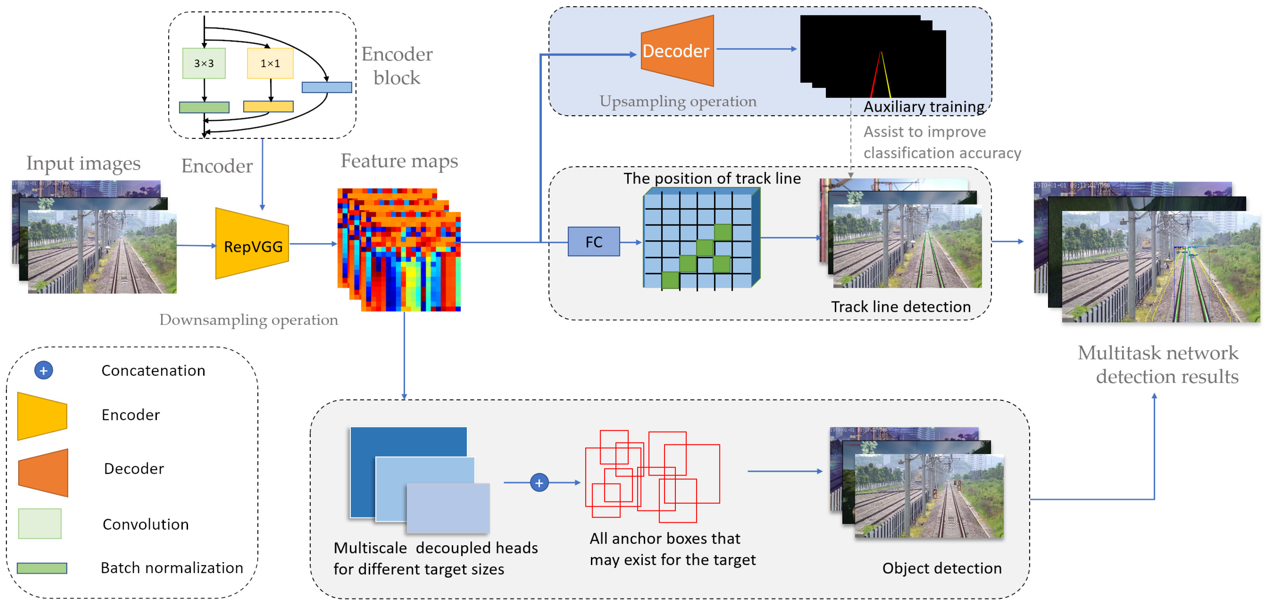
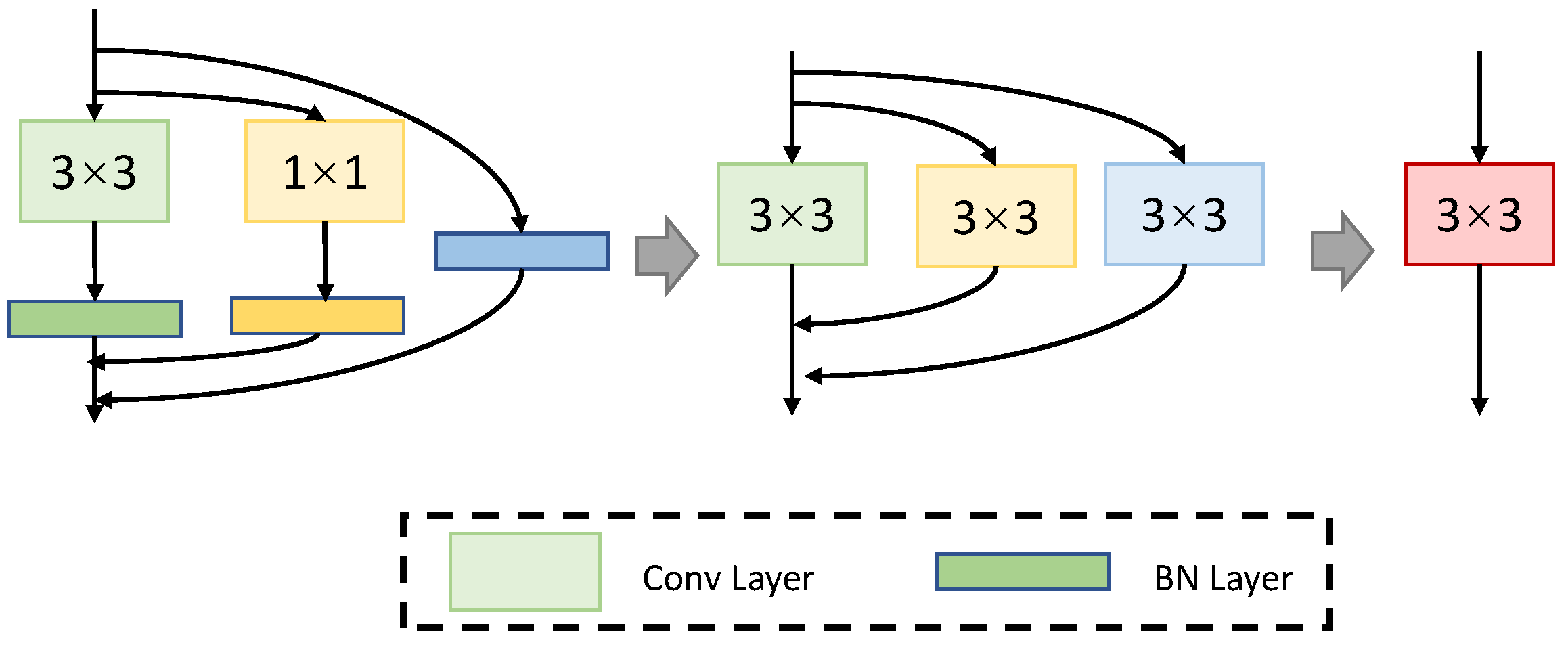
In this part, we go through the whole system used in our work from the backbone, neck, and head parts. We designed a network that contains one shared encoder and two subsequent decoders to solve specific tasks. There are no complex and redundant shared blocks between different decoders, which reduces computational consumption and allows our network to be easily trained end-to-end. The backbone network is used to extract the features of the input image. The neck is used to fuse the features generated by the backbone. Different decoders perform lane line detection and obstacle detection, respectively. Our backbone network used RepVGG [26], which adopted the idea of structural reparameterization to improve the speed and accuracy of the network. The structural reparameterization is shown in Figure 3.

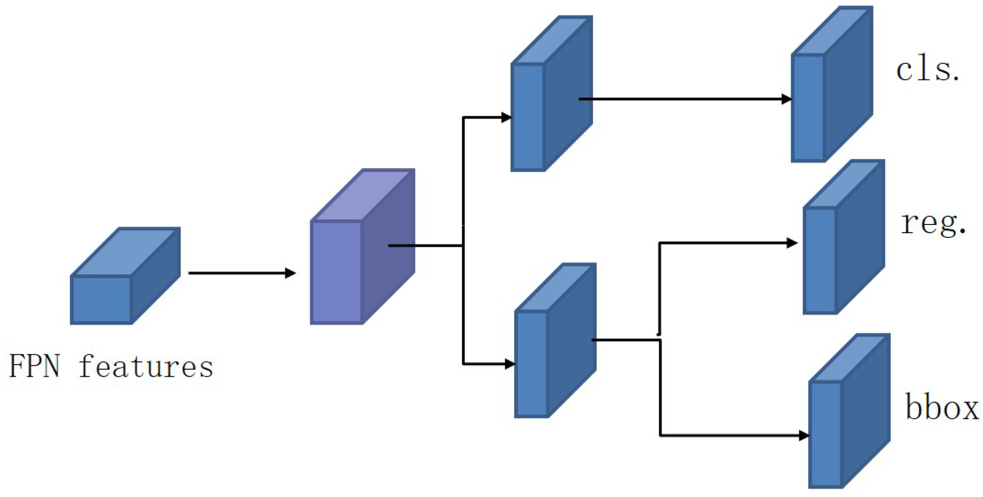
The target obstacle detection network and the train track line detection network share the backbone network which uses structural reparameterization. In the design of the head network used to detect objects, considering that the two tasks of target detection and target classification have different focal points and interesting parts, our network selects the decoupling head which is shown in Figure 4. Considering that the anchor-frame-based method not only increases the complexity of the detection head, but also needs to migrate the prediction frame generated in the detection to the GPU when generating a large number of prediction frames, the application of some edge devices can lead to unsupported device performance and cannot be used in the actual landing scene. The anchor-frame-based target detection algorithm is also easily affected by the preset anchor frame. At the same time, based on the accuracy of small target detection in the detection process and the lightweight requirements of the target detection algorithm when the algorithm is deployed, the target detection network in this paper adopted an anchor-free target detection algorithm to improve the coupling degree of the target detection algorithm to a greater extent and enhance the generalization performance of object detection results on small object data.

In the process of intrusion detection, it is not only necessary to find the location and type of the obstacle, but also to clarify the location of the obstacle. If the obstacle is in the safe area, it is not necessary to issue an alarm frequently to affect the train staff. Furthermore, if the obstacle is in the alarm area, different levels of alarms need to be issued based on the intrusion degree of the obstacle. Therefore, the network needs to establish the encroachment area by detecting the track line and performs the expansion processing as needed based on the coordinates of the detected track line. For the segmentation algorithm, if the size of the lane line image is $H\times W\times C$, then the $H\times W\times (C+1)$ classification problem needs to be dealt with when performing the segmentation. However, the slender structure of the lane line occupies a small proportion of the overall image. Pixel classification will generate a lot of unnecessary burdens and have a great impact on network performance.

Therefore, based on the special structure of the track line, the row anchor method proposed in [19] was adopted. The line classification method is used to judge whether the line has a track line on some preset lines. Line classification is a line direction selection strategy that only needs to deal with the classification problem on a given row. The classification problem on each row is w-dimensional. Therefore, the original classification of the whole image becomes a classification problem based on a given line, and since the positioning on each line can be manually set, the size of h $(h\ll H)$ can be set as needed, which greatly reduces the amount of network computation.

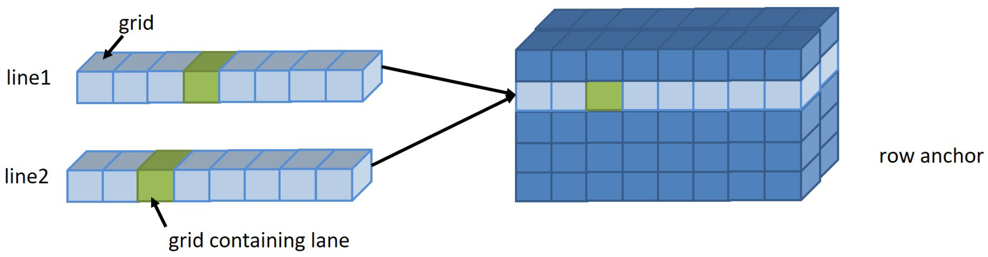
Considering that the track line itself has a certain thickness, a certain track line in a row can be regarded as a whole and can be divided into a grid. The network performs classification algorithm training and infers where this grid is located to determine where the track lines are located. Therefore, the network only needs to select the corresponding row anchor, whose schematic diagram is Figure 5, in the given row anchor, when classifying and dividing the data in each row into corresponding grids, whose number is w $(w\ll W)$. Considering that there may be no track line in the target row anchor, one-dimensional data are added to indicate that the row has no lane lines, and the number of grids is $(w+1)$. So the number of classifications that the network needs to perform is $(h\times (w+1)\times C)$, which can greatly reduce the computational complexity of the network. At the same time, to improve the detection speed, the segmentation method is used to learn the shape, structure, and position distribution of the rail area in the network only during training. The segmentation result is classified based on the row anchor to determine the grid where the rail exists.

3.2. New Formulation for Multitask Learning

The formulation for obstacle detection. The detection loss $L_{det}$ is a weighted sum of classification loss, object loss, and bounding box loss as follows:

$$L_{det}={\alpha }_1{L}_{cls}+{\alpha }_2{L}_{obj}+{\alpha }_3{L}_{box}$$

(1)

where $L_{cls}$ and $L_{obj}$ are utilized to reduce the loss of well-classified examples, thus forcing the network to focus on the hard ones. ${\alpha }_1$, ${\alpha }_2$, and ${\alpha }_3$ are coefficients of these loss functions. $L_{cls}$ is used for penalizing classification and $L_{obj}$ for the confidence of one prediction. All of them use BCEWithLogitsLoss, whose formula expression is:

$$L_n=-y_{n}log(\sigma (x_n))+(1-y_n)log(\sigma (1-x_n))$$

(2)

where n represents the number of labels predicted per batch, and $\sigma (x_n)$ can use formula $\sigma (x)=\frac{1}{1+{exp}^{-1}}$ to map x to the interval (0, 1). $L_{box}$, which is calculated by IoU, represents the intersection loss between the predicted box and the ground-truth box.

The formulation for line detection. For the lane line detection loss, the loss function generally consists of the loss of classification and the loss of segmentation. In order to better allow the network to learn the structural features of the lane lines and make sure that a relatively continuous track line maintaining a linear trend is identified, an additional structural loss was added. The loss function of the lane lines was as follows:

$$L_{line}={\beta }_1{L}_{class}+{\beta }_2{L}_{str}+{\beta }_3{L}_{seg}$$

(3)

where $L_{class}$ represents the loss of classification, $L_{str}$ represents the structural loss used to constrain track line shapes, and $L_{seg}$ represents the loss of segmentation. ${\beta }_1$, ${\beta }_2$, and ${\beta }_3$ are coefficients of these loss functions. In the classification loss, X is used to represent the input image, and $f^{(i,j)}$ is used to represent a classifier that can find the grid position where the ith lane is located from the jth row anchor. As a result, $P_{i,j,:}=f^{(i,j)}(X)$ represents the probability that each grid in the jth row anchor had the ith lane, and there are w grids in total. Moreover, $T_{i,j,:}$ indicates whether there is a lane line in the jth row anchor and the grid position where the lane line is located. Both $P_{i,j,:}$ and $T_{i,j,:}$ are $(w+1)$-dimensional (a grid is used to indicate that the row has no track lines) vectors that satisfies one-hot encoding. We can get the loss function as follows:

$$L_{class}=\sum _{i=1}^C\sum _{j=1}^h{L}_{CE}(P_{i,j,:},T_{i,j,:})$$

(4)

where $L_{CE}$ represents the cross-entropy loss used here. According to this function, the probability distribution of all positions on each row of anchor points can be predicted based on the global features. Therefore, the correct location can be selected based on the probability distribution.

In addition to the classification loss, two loss functions are proposed to model the positional relationship of the lane line points. Because the lane lines are continuous, even if it is a curve, it can be approximated as a straight railway from a distance. Therefore, the lane lines between adjacent row anchors need to be close to each other. Furthermore, the distribution of the classification vector on the adjacent row anchors needs to be constrained to ensure that the predicted probabilities of the two adjacent row anchors are as close as possible, thereby ensuring the smoothness of the overall line. The predicted similarity loss function is as follows:

$$L_{sim}=\sum _{i=1}^C\sum _{j=1}^h{\parallel P_{i,j,:},P_{i,j+1,:}\parallel }_1$$

(5)

where $P_{i,j,:}$ represents the probability that each grid in the jth row anchor has the ith lane. To account for the shape, the position of the lane on each row anchor needs to be calculated. Furthermore, the track line position is obtained from the classification prediction by finding the maximum response peak. Substituting differentiable $softmax$ for $argmax$ can get the second-order difference equation constraint $L_{shp}$, which is obtained to ensure that the overall detected track line structure is relatively smooth and the slope is relatively similar. The formula expression is:

$$L_{shp}=\sum _{i=1}^C\sum _{j=1}^{h-2}{\parallel (LO{C}_{i,j}-LO{C}_{i,j+1})-(LO{C}_{i,j+1}-LO{C}_{i,j+2})\parallel }_1$$

(6)

where $LO{C}_{i,j}={\sum }_{k=1}^{w}k\dot{P}ro{b}_{i,j,k}$ represents the expected value that the jth orbital line in the ith row anchor appears in the kth grid. $Pro{b}_{i,j,:}=softmax{P}_{i,j,k}$ in $LO{C}_{i,j}$ is used as an approximation which chooses the probability of occurrence of lane lines in each grid instead of where the track lines are located.

Based on the rail shape constraints and the rail position similarity constraints, the rail structural loss can be obtained:

$$L_{str}={\gamma }_1{L}_{sim}+{\gamma }_2{L}_{shp}$$

(7)

where ${\gamma }_1$ and ${\gamma }_2$ represents coefficients of different loss functions.

In addition to the $L_{class}$ and $L_{str}$ introduced above, we used the cross-entropy loss as the $L_{seg}$. The loss function of the lane line detection problem can then be obtained.

The formulation for the whole network. In the multitask learning process, the learning speed of different tasks is different. Based on the same input feature representation, some tasks have a low learning difficulty and fast convergence speed, while some tasks have a high learning difficulty and slow convergence speed. When the learning speed of tasks is unbalanced, it is easy to cause tasks with fast learning speed to dominate the learning process of the model, resulting in the phenomenon of self-reinforcing, which leads to the insufficient representation ability of the model and affects the results.

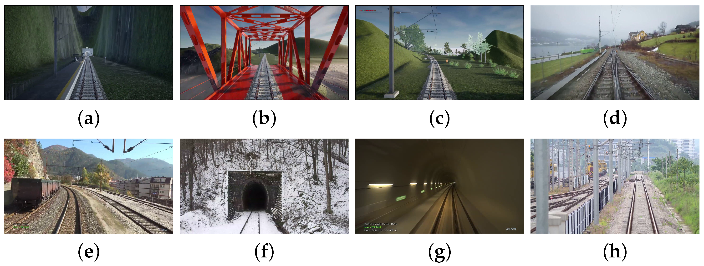
Due to the particularity of railway scenes, there are small target obstacles in both obstacle detection and track line detection tasks. Most of the pixels belong to the background area, and the target obstacles and track lines only occupy a very small part of the pixel area. At the same time, combined with the particularity of railway scenes, we pay more attention to medium- and long-distance obstacles during detection, which are more difficult to classify. These belong to the common features of the different tasks of this work. The labeled data can be seen in Figure 6. Therefore, the target detection task has problems such as unbalanced proportion of obstacle categories and unbalanced sample distribution, since the obstacle detection work needs to be able to detect all possible target obstacles in the area, and the track line detection work only needs to identify and extract the two rail lines of the current train running. Because there are position offsets of the train track lines collected in different videos, the track line detection task also has the problem of unbalanced sample distribution when performing line classification.

Multitask networks need to study how to reasonably use the characteristics of different tasks to adjust the importance of tasks, so that the importance of tasks matches the update degree of the model parameters. Then, it can ensure the learning speed remains relatively balanced, and alleviate the problem of task advantages. Based on this, we propose a new calculation method, which dynamically adjusts the coefficients of the loss function of different tasks according to the number of categories and the difficulty of sample classification for different tasks.

When designing the task, we paid more attention to the samples with low confidence in the task, which are prone to misclassification during the training process and challenge the model. We used $-log(p)$ as a judgment parameter for the difficulty of training samples, in which p references the probability that the network predicts this task objective correctly. Because the confidence range of p is (0,1], the more difficult the sample is to be predicted, the smaller the $log(p)$ is, and the larger the $-log(p)$ is. At the same time, we also considered the impact of negative samples on the results and used $(1-p)$ to represent the proportion of negative samples in the task weight. So the coefficient expression formula was:

$$Cc=-{(1-p)}^{\theta }log(p)$$

(8)

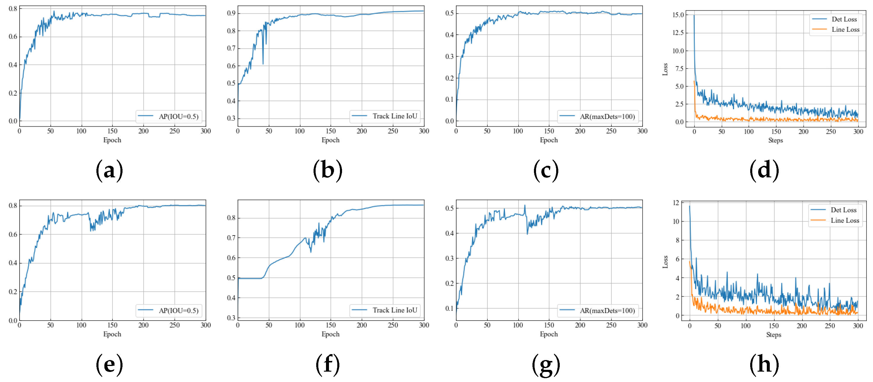
where $\theta$ was set to 2. As shown in Figure 7d, the line detection task is relatively simpler and has a faster convergence speed. In order to be able to balance two different tasks, it is necessary to relatively balance the two different tasks through the task coefficient. Therefore, the task coefficient designed above was substituted into the multitask network adaptive loss function formula $L(t)={\sum }_i{w}_i(t)L_i(t)$. The overall multitask network task formula was:

$$\begin{array}{cc}\hfill L_{total}(t)& =log(-{(1-p_{det}(t))}^{\theta }log(p_{det}(t)))L_{det}\hfill \\ \hfill & +log(-{(1-p_{line}(t))}^{\theta }log(p_{line}(t)))L_{line}\hfill \end{array}$$

(9)

Figure 7h shows the loss function results after the multiobjective coefficient trade-off. The comparison of the training results proves that the algorithm proposed by this network is beneficial to trade-off tasks with multiple objectives. Weighted by this coefficient, different tasks can converge at a relatively balanced rate.

4. Experiments

4.1. Datasets

Different from the automatic driving scene of a car, a train track line is more slender. Due to the faster train speed, it is necessary to detect farther obstacles and face the challenge of smaller target obstacles. There are no publicly available datasets in this scenario.

Since the installation of obstacles during the actual operation of a train would pose a safety threat to the train, the dataset used in this experiment was composed of real train operation data actually collected in a test field scenario, simulated data, and network crawling barrier-free train-operation monitoring data. In the simulation data, in order to make the scene picture more realistic, we used the Unreal Engine with real-time rendering capabilities, a spline mesh component to make rails, a spline component to set the train trajectory, and controlled the train to move along the set trajectory at runtime. We also bound the camera to the appropriate position of the locomotive to capture the scene while the train was running and used Unreal Engine’s terrain system, landscape and vegetation system, and foliage to create terrain and vegetation environments. Finally, we used existing animal models and character models to create rich obstacle types.

The test site data and simulation data aimed to obtain more active obstacle data, such as animals and people. The web crawling data aimed to obtain more real scene data under climatic conditions. In the proving ground scenario, the obstacles that were to appear when the train was running included people, branches, and a suitcase, which was used to replace a stone. The obstacles in the simulated data were persons and animals, including cows and horses. In the data scraped from the web, obstacles included people on a platform, traffic lights, tunnel entrances, and oncoming trains. The time in our dataset included days and nights. The weather conditions in our dataset included sunny, rainy and snowy days. The terrain of the dataset included plains, trees, mountains, stone bridges, steel bridges, etc. Some dataset pictures are shown in Figure 8.

Based on the video, one frame was extracted every 1000 frames, and the data with low imaging quality or too-repetitive scenes were removed. A total of 2400 day and night data were obtained. These data were randomly divided according to the ratio of 8:1:1. The dataset consisted of 1944 training sets, 216 validation sets and 240 test sets.

4.2. Ablation Study

In this section, we verify our method with several ablation studies. Our training settings were mostly consistent from baseline to final model. We trained the model for a total of 300 epochs and 5 epochs of warm-up on our dataset. We used the stochastic gradient descent (SGD) for training. We used a learning rate of lr × BatchSize/32, an initial lr = 0.01, and a cosine lr schedule. The weight decay was 0.0005 and the SGD momentum was 0.9. The input size was evenly drawn with 32 strides. All algorithms were trained on an RTX 3090 and the inference on a Tesla P40. The experiments were all conducted with the same settings. In order to facilitate the comparison, we used the segmentation branch to calculate mIoU when testing the network in this paper, and the rest of the indicators were calculated after canceling the segmentation branch.

Order. Although the network design appears to be designed in parallel, in actual network operation, the network is executed in a serial manner. Therefore, the order in which the two branches are designed in the head area also has a certain impact on the network results. In this part, we executed the lane line detection head and the target detection head, respectively, and compared the network results. The results are shown in

Table 6. Comparison of order with lane line detection head first or target detection head first.

Order	Accuracy (%)	mIoU (%)	Top 1 (%)
Lane-first	69.6	59.6	52.3
Detect-first	66.0	60.53	51.78

. There was no segmentation branch in the actual reasoning, and the lane line recognition effect could only be judged by the classification result. The lane line priority scheme could obtain a better prediction accuracy(+3.6%) and classification accuracy (+0.6%) and had better indicators in the test stage. So in the network design, we chose the lane-first order.

Backbone. In addition to RepVGG, we also tested this experiment on the now commonly used YOLO series backbone networks ResNet50 and DarkNet53. The experimental results are shown in

Table 7. Comparison of networks with ResNet50, DarkNet53, and RepVGG as the backbone.

Backbone	Accuracy (%)	mIoU (%)	Top 1 (%)	FPS (%)
ResNet50	35.8	52.95	50.8	66
DarkNet53	64.0	62.21	51.3	67
RepVGG	69.6	59.6	52.3	52

. The experiments showed that the target detection algorithm using RepVGG had the best performance, and the lane line detection performance obtained by using DarkNet53 was the best. However, as mentioned above, practical reasoning was more focused on detection and classification metrics. The backbone network based on RepVGG had the best detection indicators and classification indicators, so we chose RepVGG as the backbone network of the network.

IoU Loss. In addition to the above two differences, different bounding boxes can be used to predict the loss during detection, and different calculation methods of intersecting the predicted box and the real box can be used. There were different results in the small-target calculation process, as shown in

Table 8. Comparison of $L_{box}$ with different IoU losses.

${\mathit{L}}_{\mathit{box}}$	Accuracy (%)	mIoU (%)	Top 1 (%)
$L_{IoU}$	69.6	59.6	52.3
$L_{DIoU}$	69.5	61.3	51.46
$L_{CIoU}$	67.5	56.42	51.72
$L_{EIoU}$	71.1	60.06	51.07

. $L_{EIoU}$ had the highest detection accuracy, and $L_{IoU}$ had the highest classification accuracy. Comparing the difference between the two, $L_{EIoU}$ was slightly more advantageous than $L_{IoU}$. Taking the above information into consideration, we used $L_{EIoU}$ as $L_{box}$.

Weight. After selecting the type of bounding box, different weights of $L_{box}$ will have different effects on the results. For the given weight setting, we chose 2, 5, 8, and 10 for comparison and experimentally chose the most favorable weights for the results. The results are shown in

Table 9. Comparison of weights of object detection loss.

Weight	Accuracy (%)	mIoU (%)	Top 1 (%)
2	61.8	70.22	89.96
5	71.1	60.06	51.07
8	58.9	63.6	89.04
10	48.3	81.52	89.16

. Through experiments, we can see that when the weight is 5, the best detection effect can be achieved. When the weight is 2, the best lane line recognition effect can be achieved. Comparing the difference between the two, when the weight is 5, it is 9.3% more than when the weight is 2, but it is 10.16% less when performing the segmentation operation and 38.89% less when classifying the lane lines, which is much larger than the difference in classification results. In general, a weight of 2 could achieve better results. The parameters with a weight of 2 were subsequently selected.

Finally, we compared our designed task-adaptive-based multitask loss function with a simple summation loss function, and the results are shown in

Table 10. Comparison of the different methods for multitask loss.

Method	Accuracy (%)	mIoU (%)	Top 1 (%)
Add directly	61.8	70.22	89.96
Ours	68.6	73.69	89.79

. The weight calculation used had a good index improvement in object detection and lane line segmentation. The results prove that our proposed task-based multiobjective adaptive algorithm has a good representation of the dataset of this paper.

In general, the algorithm in this paper prioritized lane line detection during code execution, selectd RepVGG as the network backbone, used $L_{EIoU}$ as $L_{box}$, with a weight of 2, and adopted the dynamic task-adaptive-based multitask loss function proposed in this paper when calculating the multitask loss function.

4.3. Visualization

The visualization of this network on the test set is shown in Figure 9.

4.4. Comparison to Other Methods

In this section, we compare the results of this network and other object detection or lane line networks running on our dataset. In these experiments, we used RepVGG as our backbone, a head-first lane line detection as the head network order and used $L_{EIoU}$ as $L_{box}$. For the obstacle detection, three methods were used for experimental comparison. The results are shown in

Table 11. Comparison with the results of other target detection networks.

Method	Size	GFlops	Params (M)	Accuracy (%)	FPS
ATSS [27]	640	205	32	56.2	12
YOLOX-s [28]	640	27	9	53.7	69
YOLOv7-s [29]	640	104	37	65.7	56
Ours	640	128	85	68.6	52

. Although the method proposed in this paper is not as real-time as YOLOX and YOLOv7, it can also meet the real-time requirements while the frame rate of the video is 25 FPS. Furthermore, the method used in this article achieved the best results in detection accuracy, with a 2.9% improvement compared to YOLOv7, which is the latest work in the YOLO series.

For the lane line detection network, we used the segmentation network for the experimental comparison. In this comparative experiment, FPS was calculated with a segmentation branch. The results are shown in

Table 12. Comparison with the results of other segmentation networks.

Method	Size	GFlops	Params (M)	mIoU (%)	FPS
Deeplabv3 [30]	416	1021	63	33.12	16
PSPNet [31]	416	619	664	57.55	13
CCNet [32]	416	804	427	58.7	9
DANet [33]	416	1110	2339	43.44	10
ISANet [34]	416	386	252	42.38	27
Ours	640	128	85	73.69	40

. Table 12 also proves that the slender structure of the track line is not suitable when applying a pure segmentation algorithm.

From Table 11 and Table 12, it can be seen that although our method is insufficient in FPS compared with other YOLO methods, it has better performance in both accuracy and mIOU. Regarding computational efficiency, because multitask networks need to perform more task runs than single-task networks, the number of model parameters and the model complexity are increased. However, although the number of model parameters is increased, for new tasks with little data, the cold start problem is also solved. The potential reason is that different tasks have different noises. Assuming that the noises of different tasks tend to be in different directions, learning together offsets some of the noise to a certain extent, making the learning effect better and the model more robust. In addition, the multitask method adopts a shared encoder structure and different tasks affect the feature generation part. As a result, the associated multitask learning can achieve a better generalization effect than single-task learning, and reduce the possibility of model overfitting. Through the intersection and union of multiple different task solution spaces, the multitask solution space is supplemented and generalized to obtain a more representative solution space. Therefore, the multitask learning performance is better than the single-task learning one.

In general, the multitask network proposed in this paper can achieve more advantageous experimental results than those of the single-task network. At the same time, the weight of the task-adaptive loss function proposed in this paper can also improve each individual task.

5. Conclusions

In this paper, we proposed a multitask learning network that was used for railway obstacle intrusion detection. The network could detect obstacles appearing in front of the train in real time and could identify the rail track line. It could perform obstacle recognition and multilevel warning functions even if the track line was blocked, so that railway operations’ risks were reduced. By using the track line detection algorithm based on line classification, our work made up for the shortcomings of using a segmentation method for track line detection, and the segmentation results were greatly improved. We also designed a multitask loss function coefficient for balancing different tasks’ complexity, which helped the network better perform different detection tasks.

The current network had better processing capabilities for straights and gentle curves. Future work may focus on strengthening the processing of curves and improving the robustness of the network under different rail conditions.