A Unified FPGA Realization for Fractional-Order Integrator and Differentiator

Abstract

This paper proposes a generic FPGA realization of an IP core for fractional-order integration and differentiation based on the Grünwald–Letnikov approximation. All fractional-order dependent terms are approximated to simpler relations using curve fitting to enable an efficient hardware realization. Compared to previous works, the proposed design introduces enhancements in the fractional-order range covering both integration and differentiation. An error analysis between software and hardware results is presented for sine, triangle and sawtooth signals. The proposed generic design is realized on XC7A100T FPGA achieving frequency of 9.328 MHz and validated experimentally for a sine input signal on the oscilloscope. The proposed unified generic design is suitable for biomedical signal processing applications. In addition, it can be employed as a laboratory tool for fractional calculus education.

1. Introduction

Fractional calculus describes the noninteger-order differentiator and integrator, where the order can be real, complex, or rational [1]. Fractional calculus has become more popular and is widely used because of its flexibility, tunability, memory dependency and, hence, ability to model systems [2,3]. Engineering applications of fractional calculus include: bioengineering [4], control [5], filters [6], oscillators [7], energy [8], encryption [9], and chaos [10]. The most common fractional operators are the Grünwald–Letnikov (GL), Caputo, and Riemann–Liouville (RL) [11]. The GL definition, which is an extension of the Euler method, is the primary focus of this work.

The GL definition is given by [3]:

$${}_a^{GL}{D}_t^{q}x\left(t\right)=\underset{h\to 0}{lim}\frac{1}{h^q}\sum _{j=0}^{\lfloor (t-a)/h\rfloor }{w}_j^{\left(q\right)}x(t-jh),$$

(1a)

$$w_0^{\left(q\right)}=1,w_j^{\left(q\right)}=\left(1-\frac{q+1}{j}\right)w_{j-1}^{\left(q\right)},j=1,2,3,\cdots$$

(1b)

where $w_j^{\left(q\right)}$ are the binomial coefficients, h is the step size, and q is the fractional order. The binomial coefficients act as damping factors that result in the stability and accuracy of the GL method [12]. The summation in the definition lends itself to adaptation for use in a computer numerical solver [13] and digital hardware realization. The concept of the short memory principle was proposed as follows [3]:

$${}_a^{GL}{D}_t^{q}f\left(t\right)\approx {}_{t-L}^{GL}{D}_t^{q}f\left(t\right),t>a+L$$

(2a)

$${}_{t-L}^{GL}{D}_t^{q}x\left(t\right)=\frac{1}{h^q}\sum _{j=0}^L{w}_j^{\left(q\right)}x(t-jh),$$

(2b)

where L is the window size, which limits the memory dependency to a finite window, including a fewer number of the previous iterations [3,14], resulting in another form for the GL operator (2b), which can be implemented on hardware based on the window size L.

The error calculation depends on the difference between the general form of GL (1a) and the approximated equation with window L. The upper bound of the error, which is a result of the approximation (2b), is given as follows [15]:

$$\Delta \left(t\right)=\left|{}_a^{GL}{D}_t^{q}x\left(t\right)-{}_{t-L}^{GL}{D}_t^{q}x\left(t\right)\right|\le \frac{M{L}^{-q}}{\left|\mathsf{\Gamma }\right(1-q\left)\right|},$$

(3)

where $a+L<t<b$ with window L, $\left|x\right(t\left)\right|<M$, when $a<t<b$ for the infinite definition in (1a), where a is the start point and b is the end point of the interval under investigation, and t lies in it. Different applications require several values of fractional orders to perform integration and differentiation. This needs more flexibility in changing the order in hardware, without redesigning the whole architecture of calculating the response of a fractional-order system.

FPGAs have an important role in digital communications and complicated systems because of their characteristics such as flexibility due to the predesigned configurable logic blocks (CLB) and a high speed, up to hundreds of megahertz (MHz) [16]. Unlike application specific integrated circuits (ASIC), the design-implement-test-debug cycle may take only hours on an FPGA while on ASIC it can take months. Therefore, the modification in the design is easier [17]. Furthermore, FPGAs have intrinsic advantages such as a large capacity, real-time computation, cheap cost and low power consumption. Therefore, FPGAs can be used in high-speed industrial applications that meet the intended criteria and match the parallel structure.

The implementation of the GL definition on FPGA has been attempted many times in the literature. The advantages of the GL over the Caputo definitions in digital realization include a smaller area, better performance, and avoiding the complexity of implementing sinc or Gaussian functions, unlike Caputo’s implementation [18]. Additional advantages for the GL over the Caputo and RL definitions in digital applications are the GL’s discretized form and the short memory principle [18]. These digital realizations still lacked generality of the hardware design and had limited ranges for the fractional order q. Most of these works relied on software to calculate $h^q$ and binomial coefficients $w_j^{\left(q\right)}$ and stored them in lookup tables (LUT). Furthermore, some practical applications need only differential operations, such as chaotic systems [19]. Other applications use integral operations [20] such as the damped oscillator system and other control systems. Some applications use both diff/int operations, such as fractional-order proportional integral derivative (FOPID) controllers [21], where reliable architectures and generic designs are needed. In [22], the fractional-order operator was implemented on hardware and employed in different applications such as the generation of chaotic systems. A comparison between different approaches for integrator and differentiator operators of the GL definition was proposed in [23]. The LabVIEW software tools were used to produce the RTL code implementing the fractional-order integrator and differentiator using GL as proposed in [24]. In [25,26], a generic GL definition with a fixed-window approach employed in a chaotic system was proposed. In [27], a generic hardware realization for the GL-based differentiator was proposed. This paper proposes a generic hardware design of a GL-based differentiator and integrator, which involves an improvement in the range of order q and a decrease in the reliance on software for the calculation of different parameters of GL. The proposed design is independent of changes in the value of q within the covered range and does not require fixed-step increments of q. The proposed design demonstrates its approximation efficiency through an error analysis between software and hardware results achieving a maximum error of $0.05$ at $q=0.9$. The proposed design achieves good hardware utilization with a frequency of $9.328$ MHz.

The rest of this paper is organized as follows: Section 2 compares different works which implemented the GL operator on FPGA. Section 3 shows the hardware architecture of the proposed generic fractional-order differentiator and integrator design. Section 4 provides the FPGA results and experimental validation. Finally, the concluding remarks are summarized in Section 5.

2. Literature Review of GL-Based Fractional Operators Implementations

The fractional-order operators were implemented on FPGA by several works with different approaches including: fixed-window [22], fixed-linear approach, piecewise quadratic (PWQ) and piecewise linear (PWL) [23]. The fixed-window approach was designed to calculate a fixed number of binomial coefficients and obtain the output of the GL definition only for a differentiator, based on the length of this window as in [22]. Different chaotic systems were implemented based on the proposed GL hardware design in [22]. Another hardware design for Caputo and GL definitions realizing different derivative orders was proposed in [18]. Moreover, a new implementation of the GL operator based on the linear approximation technique was proposed in [28]. Additionally, FPGA implementations of a fractional-order differentiator and integrator based on a GL operator were introduced in [23]. Two approaches were developed based on quadratic and piecewise linear approximations. The transfer functions of different fractional-order applications were implemented. The applications included a Heaviside’s inductor-terminated lossy line system, damped oscillator and fractional-order controller.

In [29], fixed-window and linear approximation approaches were introduced to implement differential and integral operators to reduce the memory dependency of the fractional-order operators. The two approaches were used as building blocks to implement a fractional-order proportional integral derivative (FOPID) controller on an FPGA. The GL-based FPGA implementation of different families of fractional-order chaotic oscillators was introduced in [30]. The proposed architecture used a stored value of coefficients in a read-only memory to be employed later in the calculations.

In [25], a generic GL hardware implementation was proposed with a modified fixed-window approach and employed to implement a chaotic system. The design calculated the binomial coefficients and the $h^q$ on the hardware platform, for the range q∈$[0:1.5]$. The range of order q was quite wide. However, it was limited for differentiator operations, and $h^q$ was limited to powers of 2. Another generic hardware implementation for the GL operator with different derivative fractional orders was proposed in [26]. A multiscroll fractional-order NEW-SPROTT-41 system was implemented using the proposed GL architecture. In [27], a generic design for the GL based differentiator was proposed, realizing a reconfigurable fractional-order chaotic system. The design achieved the generality of differentiator order in the range of q∈$[0.7:1]$. However, it had a limited range of order q, and the integration operation was not mentioned.

In [31], a hardware implementation of fractional primary operators, integrator, and differentiator, on an FPGA integrated with a digital oscilloscope on the same board was proposed. The design included a module for a digital storage oscilloscope, a module for fractional operation and a PCIe module used to establish communication lines between parts of the entire system. The goal of that integration was to decrease the operating time while improving the measurement range and accuracy.

Table 1. Summary of different works on fractional-order integrator and differentiator.

Ref	Diff./Integ.		Application	Generality				Approaches	q Range	Window Size
	Diff.	Int.		${\mathit{h}}^{\mathit{q}}$		${\mathit{w}}_{\mathit{j}}^{\mathbf{\left(}\mathit{q}\mathbf{\right)}}$
				MATLAB	Hardware	MATLAB	Hardware
[22]	✓	—	chaotic systems	✓	—	✓	—	fixed window	0 ≤ $q$	20,40,30
[23]	✓	✓	fractional order systems	✓	—	✓	—	fixed-linear, fixed-quadratic and pwl	$-0.5$ < $q$ ≤ $0.5$	64,512,20
[30]	✓	—	oscillators	✓	—	✓	—	fixed window	$0.5$ < $q$ ≤ 1	256
[29]	✓	✓	FOPID controller	✓	—	✓	—	fixed window-linear	—	32,512,1024
[18]	✓	✓	—	✓	—	✓	—	fixed window-linear	—	32
[25]	✓	—	chaotic systems	—	✓	—	✓	fixed window-linear	0 < $q$ ≤ $1.5$	32
[26]	—	—	chaotic systems	—	✓	—	✓	fixed window	$0.5$ < $q$ ≤ 1	28,56
[27]	—	—	chaotic systems	—	✓	—	✓	fixed window	$0.7$ < $q$ ≤ 1	16,32
[31]	✓	✓	—	—	—	—	—	—	—	—

summarizes different previous contributions and implementations of the fractional-order GL operator on a hardware platform. Some works used software to calculate $h^q$ and $w_j^{\left(q\right)}$, changing the whole design every time q changed. Therefore, hardware is not applicable for variable orders. Other works improved the calculations of $h^q$ and $w_j^{\left(q\right)}$ on the hardware platform for specific ranges of q.

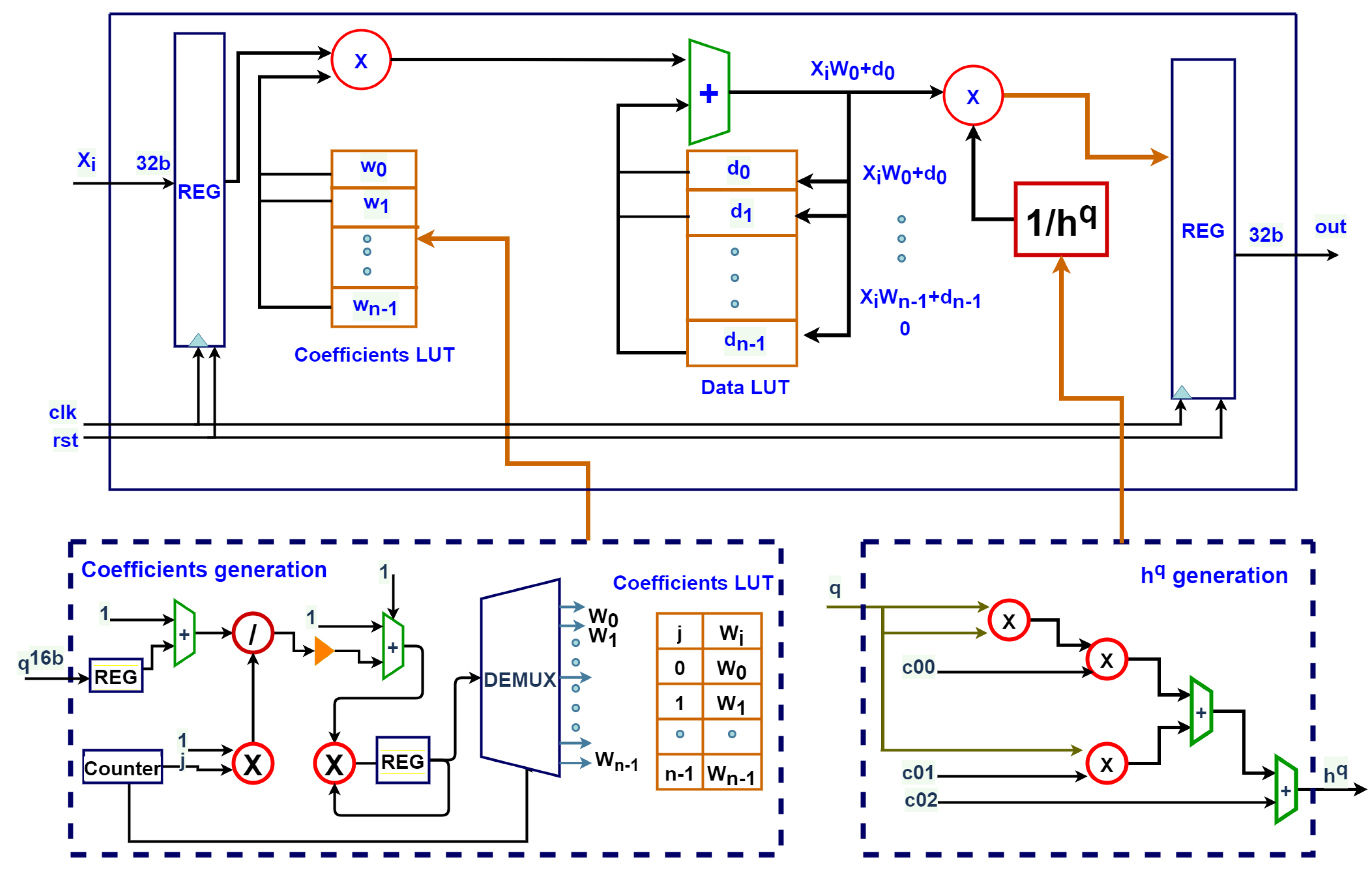
3. Proposed Generic Hardware Realization of Fractional-Order GL-Based Integrator and Differentiator

This section introduces the proposed generic implementation of integrator and differentiator of the GL operator. The proposed design generalizes the fixed-window approach introduced in [22], to include both differentiator and integrator operations.

Figure 1 shows the binomial coefficients, described by (1b), with different orders $q$ providing both differentiator and integrator for 0.4, 0.9, −0.4, and −0.9. For the differentiator case, $w_j^{\left(q\right)}$ tends to zero after a small range of iterations. Therefore, the fixed-window approach is applicable for systems that need differentiator applications. On the other hand, for the integrator case, the fixed window has a more significant error leading to an increase in the number of iterations (window size), which is a trade-off with hardware resources. Figure 2 shows the proposed hardware architecture, described in detail as follows:

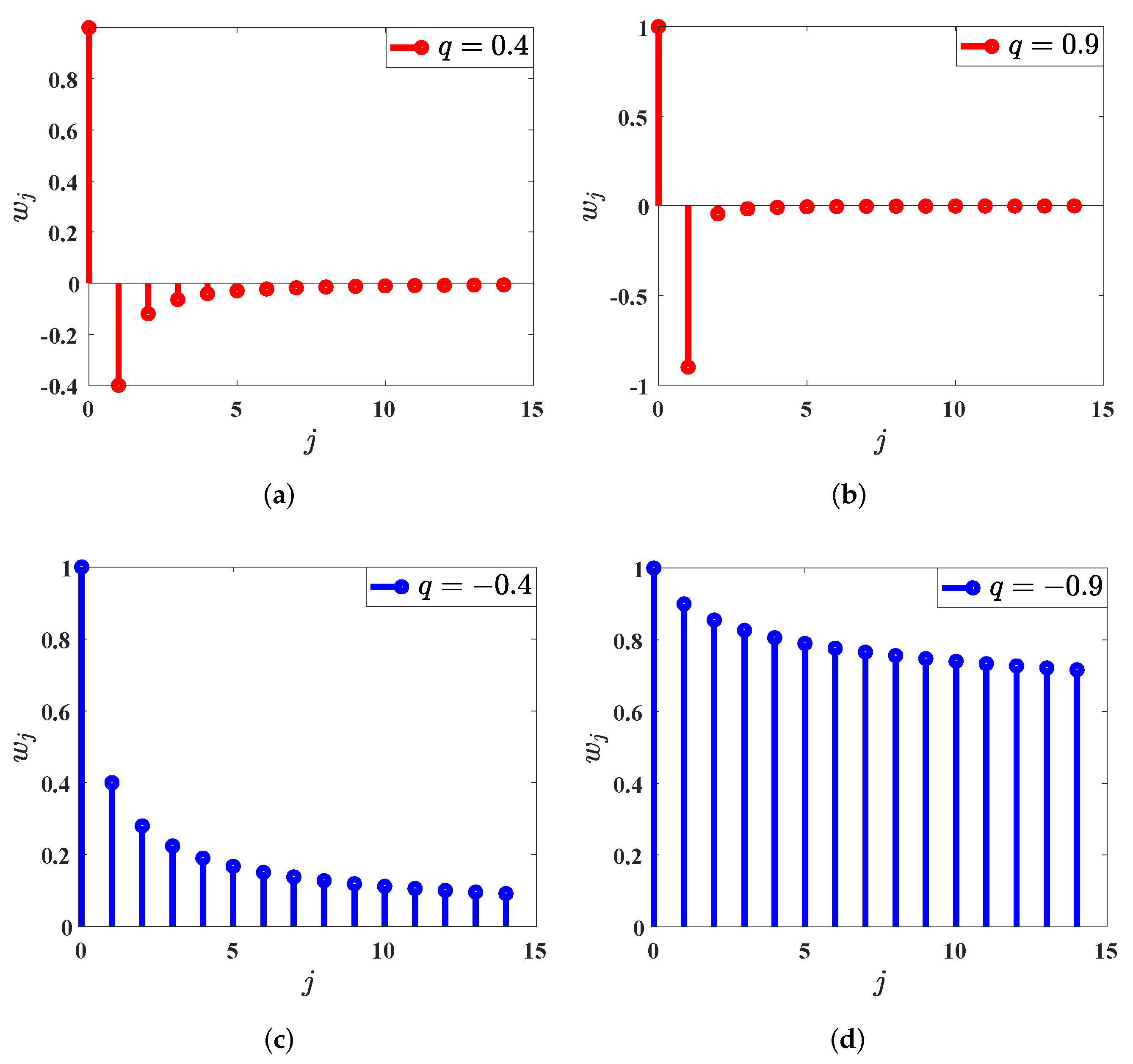
3.1. Binomial Coefficients Generation

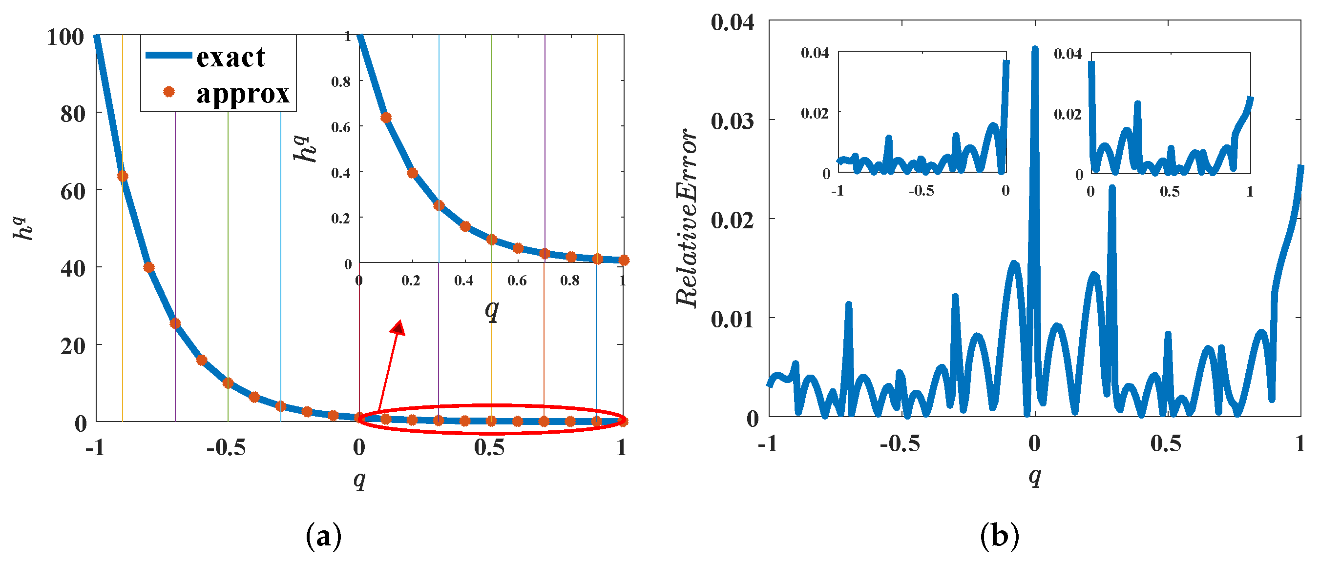
Based on (1b), the generation of binomial coefficients depends on the value of order $q$. Order $q$ is received as an input represented with a fixed-point representation as 4 bits for the integer part and 12 bits for the fractional part. Afterwards, the $q$ value is stored into a register to be used when calculating the binomial coefficient for the first iteration based on (1b), storing every coefficient in a LUT. Finally, that operation is repeated for the target window size, where the coefficients can be generated for a target window size $L$ up to 1024.

3.2.  $h^q$ Generation

The proposed design was based on a curve fitting approximation with MATLAB, to approximate the curve of $h^q$ against order $q$, in the range ∈$[-1:1]$, as shown in Figure 3a. For the negative values of $q$, the magnitude of $h^q$ reached high values. Moreover, if $q$ increased, $h^q$ got smaller with a nonuniform rate of change. On the other hand, positive values of $q$ had a regular rate of change, making the fitting process more manageable. The summed square of residual (SSE), given by (4), calculated the overall deviation of the fitting values [32,33]. The SSE was used to determine the order of the polynomial fitting for each range of the $h^q$ curve. The negative range had the highest division ratio because of the irregular change in the values of $h^q$.

$$SSE=\sum _{i=1}^{n_t}{\left(y_{exp}\left(i\right)-y_{mod}\left(i\right)\right)}^2,$$

(4)

where $y_{exp}$ is the observed data value, $y_{mod}$ is the model predicted value, and $n_t$ is the number of data points.

The proposed approach depended on dividing the range of $h^q$ into subranges as in Figure 3a. The curve of $h^q$ was divided into subcurves, each curve describing a specific range of $q$ values as illustrated using the vertical lines in Figure 3a, which was fitted with polynomial least squares [34]. According to [27], a rational curve fitting has the highest accuracy. However, it consumes the highest resources; and vice versa for a linear curve fitting. On the other hand, a quadratic fitting is the best approximation for both resources and accuracy. Inspired from [23], the curve of $h^q$ was divided into 8 intervals of different ranges of $q$. Then, the polynomial curve fitting was employed for each subrange.

Applying the fitting process on hardware imposes a limited accuracy compared to the software results. Therefore, this approach was appropriate to generate $h^q$ for a wide range of values with an accuracy of more than 96% as shown in Figure 3b. Applying the previous approach to hardware involved checking the input $q$ to determine the appropriate fitting equation. Based on the range of $q$, the coefficients of the polynomial equation of each range were determined to calculate the value of $h^q$. After the calculations of $h^q$ and binomial coefficients $w_j^{\left(q\right)}$, the calculation of (1a) was quite easier and more optimized.

3.3. Fixed-Window Hardware Implementation:

Finally, using $h^q$ and the binomial coefficients $w_j^{\left(q\right)}$ values we applied the summation of (1a) for the same window size used in generating the coefficients. The input signal or system was received as digital values represented in a fixed-point representation as 32 bits with a precision of 24 bits for the fraction part and 8 bits for the integer part. This signal was stored in a LUT. The output was represented in 32 bits to get a higher precision.

Based on the values of the rate of change for the $h^q$ curve, in each value of order $q$, the ranges of $q$ were implemented as in Figure 3a, which shows the values of $h^q$ generated by the hardware platform in the range of $q$∈$[-1:1]$ at $h=0.01$. The quadratic approximation equation is described in (5) and its hardware implementation is in Figure 2, where the ranges of order $q$ have different values of coefficients $c_{00}$, $c_{01}$, and $c_{02}$. Each range of $q$ has a specific interval in the curve of $h^q$ calculated using the second-order polynomial approximation.

$$h^q=c_{00}{q}^2+c_{01}q+c_{02}.$$

(5)

The relative error was calculated between the MATLAB values and the results generated in the approximated hardware approach for different values of $q$, as presented in Figure 3b.

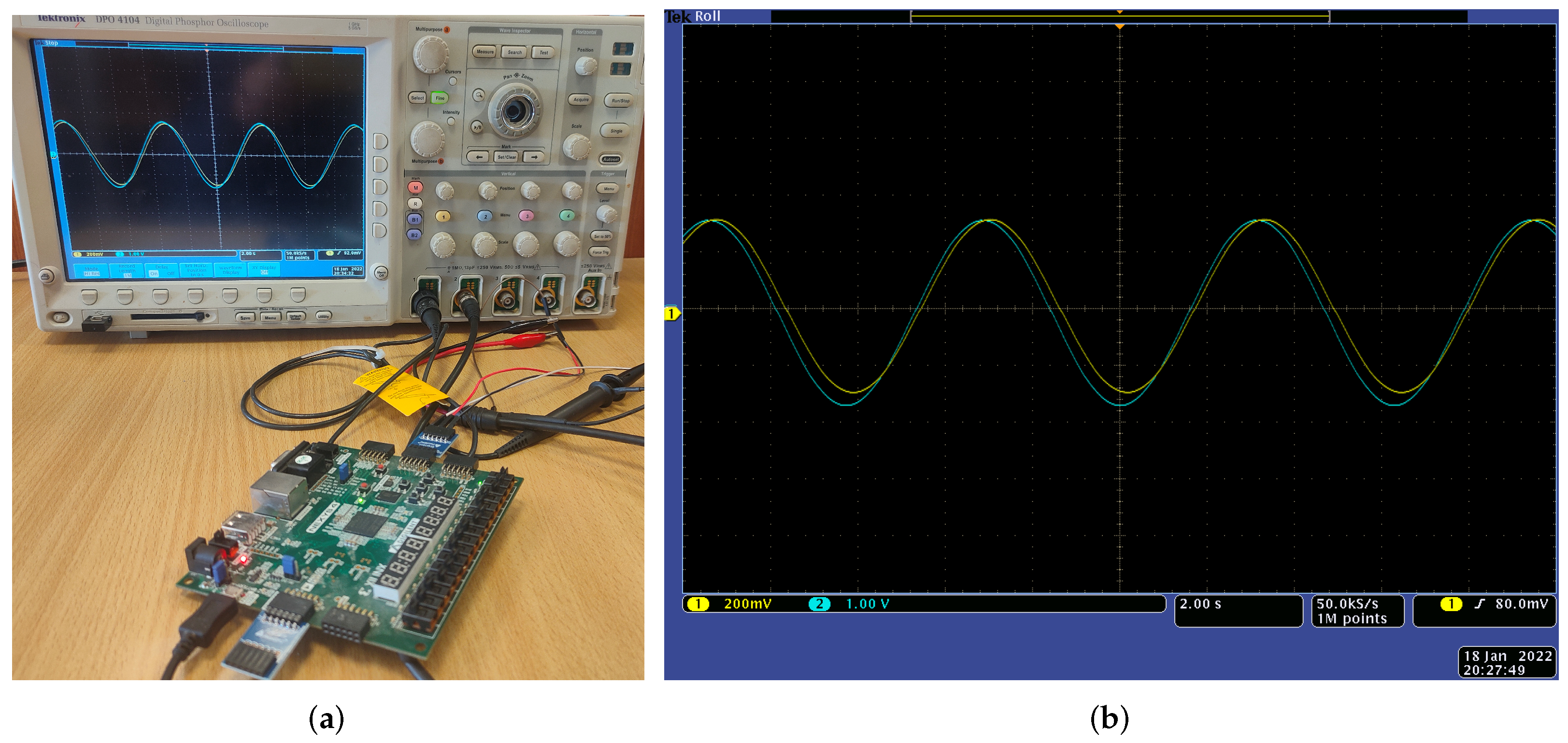
4. Results and Discussion

The testing process was done with different values of $q$ and at different window sizes, for three different input signals. The differentiator operations were tested with orders $q=0.3$, $q=0.6$, and $q=0.9$ and the integration was tested for orders $q=-0.3$, $q=-0.6$, and $q=-0.9$ with window sizes of $L=32$, $L=512$, and $L=1024$.

Table 2. The error of the proposed design results (differentiator and integrator) for a sine signal input with respect to MATLAB results.

	L = 32	L = 512	L = 1024
Derivative
Integral

shows the error of the proposed generic fixed-window approach with a sine signal as an input. The error when order $q$ is negative is larger than the error when order $q$ is positive.

Table 3. The error of the proposed design results (differentiator and integrator) for a sawtooth signal input with respect to MATLAB results.

	L = 32	L = 512	L = 1024
Derivative
Integral

and

Table 4. The error of the proposed design results (differentiator and integrator) for a triangle signal input with respect to MATLAB results.

	L = 32	L = 512	L = 1024
Derivative
Integral

show the error of the GL fractional-order differentiator and integrator of the proposed design for a sawtooth signal and a triangle signal, respectively, with different orders of $q$ and window sizes $L$.

Table 5. Comparison between the maximum errors of the proposed implementation and [29] for sine signal.

	$\mathit{L}\mathbf{=}\mathbf{32}$		$\mathit{L}\mathbf{=}\mathbf{1024}$
	$\mathit{q}\mathbf{=}\mathbf{0.9}$	$\mathit{q}\mathbf{=}\mathbf{-}\mathbf{0.9}$	$\mathit{q}\mathbf{=}\mathbf{0.9}$	$\mathit{q}\mathbf{=}\mathbf{-}\mathbf{0.9}$
The proposed Design	0.22	1.7	0.05	1.4
[29]	0.22	1.8	0.01	1.5

summarizes the values of the maximum errors for the proposed design and [29] with different $L$ and $q$ with a sine signal as an input.

The GL-defined differentiator and integrator of the proposed design hardware architecture were implemented on a Nexys-4 XC7A100T FPGA of Artix-7. Xilinx ISE 14.7 was utilized for the simulation. MATLAB software simulation was used to validate the GL design. Then, it was compared with the FPGA output. A LUT was used to store the input signal of the FPGA for the test.

Table 6. FPGA hardware resources summary on XC7A100T.

Logic Utilization	No. of Slice LUTs	No. of Slice Registers	Maximum Frequency (MHz)	DSP Multipliers
Proposed Design (L = 20)	22,968 (36%)	1072 (1%)	9.328	64 (26%)

presents the FPGA hardware resources of the proposed approach for a window size $L=20$. The proposed implementation achieves a slice utilization percentage of $36\%$, slice registers percentage of $1\%$, a number of DSPs of 64 with the utilization of $26\%$, and a frequency of 9.328 MHz. To convert the FPGA output to analog streaming to be showed on an oscilloscope device, a Pmod DA2 module was used and driven with two bits generated by the FPGA. Figure 4 shows the experimental setup and FPGA results for the generic GL design on the oscilloscope. The setup shows the output signal at a window size of 20 and the input sine signal after applying a GL integrator with order $q=-0.9$. The accuracy improves with the increase of $L$. However, the hardware resources increase at large values of $L$.

The design can be tested for any $L$ up to 1024 and is applicable for any $q$ in the proposed range. Therefore, the proposed approach can be implemented to perform integration with the accuracy presented. The proposed design provides the generality of the hardware architecture and achieves flexibility with a wide range of $q$∈$[-1:1]$ for both integrator and differentiator. The proposed implementation can be used in many applications such as encryption and biomedical signal processing applications.

5. Conclusions

A generic IP core for fractional-order int/diff of the GL operator was designed with the Verilog hardware description language. The proposed approach decreased the dependency on software and made the proposed architecture more tunable. It provided more generality in the implementation compared with previous works. Moreover, the proposed implementation proved its curve fitting approximation efficiency through an error analysis between software and hardware results. An Artix-7 FPGA board was used to test the proposed IP design at $L=20$, and the experimental results were shown on an oscilloscope. The proposed generic hardware implementation achieved a slice utilization percentage of $36\%$, a slice registers percentage of $1\%$, a DSPs percentage of $26\%$, and a frequency of 9.328 MHz. The proposed generic implementation can be employed in many applications such as dynamic encryption applications, dynamic switching and synchronization, variable-order chaotic systems, and fractional-order controller systems.

References

1. Machado, J.T.; Kiryakova, V. Recent history of the fractional calculus: Data and statistics. Handb. Fract. Calc. Appl. 2019, 1, 1–21. [Google Scholar]
2. Petráš, I.; Terpák, J. Fractional calculus as a simple tool for modeling and analysis of long memory process in industry. Mathematics 2019, 7, 511. [Google Scholar] [CrossRef] [Green Version]
3. Podlubny, I. Fractional Differential Equations: An Introduction to Fractional Derivatives, Fractional Differential Equations, to Methods of Their Solution and Some of Their Applications; Elsevier: Amsterdam, The Netherlands, 1998. [Google Scholar]
4. Kaskouta, E.; Kapoulea, S.; Psychalinos, C.; Elwakil, A.S. Implementation of a fractional-order electronically reconfigurable lung impedance emulator of the human respiratory tree. J. Low Power Electron. Appl. 2020, 10, 18. [Google Scholar] [CrossRef]
5. Xu, Y.; Li, Q.; Li, W. Periodically intermittent discrete observation control for synchronization of fractional-order coupled systems. Commun. Nonlinear Sci. Numer. Simul. 2019, 74, 219–235. [Google Scholar] [CrossRef]
6. Qiu, X.; Feng, H.; Hu, B. Fractional order graph filters: Design and implementation. Electronics 2021, 10, 437. [Google Scholar] [CrossRef]
7. Ouannas, A.; Khennaoui, A.A.; Momani, S.; Grassi, G.; Pham, V.T.; El-Khazali, R.; Vo Hoang, D. A quadratic fractional map without equilibria: Bifurcation, 0–1 test, complexity, entropy, and control. Electronics 2020, 9, 748. [Google Scholar] [CrossRef]
8. Alam, M.S.; Alotaibi, M.A.; Alam, M.A.; Hossain, M.A.; Shafiullah, M.; Al-Ismail, F.S.; Rashid, M.M.U.; Abido, M.A. High-level renewable energy integrated system frequency control with SMES-based optimized fractional order controller. Electronics 2021, 10, 511. [Google Scholar] [CrossRef]
9. Gao, X.; Yu, J.; Banerjee, S.; Yan, H.; Mou, J. A new image encryption scheme based on fractional-order hyperchaotic system and multiple image fusion. Sci. Rep. 2021, 11, 15737. [Google Scholar] [CrossRef]
10. Rahman, Z.A.S.; Jasim, B.H.; Al-Yasir, Y.I.; Abd-Alhameed, R.A. High-Security Image Encryption Based on a Novel Simple Fractional-Order Memristive Chaotic System with a Single Unstable Equilibrium Point. Electronics 2021, 10, 3130. [Google Scholar] [CrossRef]
11. Teodoro, G.S.; Machado, J.T.; De Oliveira, E.C. A review of definitions of fractional derivatives and other operators. J. Comput. Phys. 2019, 388, 195–208. [Google Scholar] [CrossRef]
12. Scherer, R.; Kalla, S.L.; Tang, Y.; Huang, J. The Grünwald–Letnikov method for fractional differential equations. Comput. Math. Appl. 2011, 62, 902–917. [Google Scholar] [CrossRef] [Green Version]
13. Loverro, A. Fractional Calculus: History, Definitions and Applications for the Engineer; Rapport Technique; Univeristy of Notre Dame, Department of Aerospace and Mechanical Engineering: Notre Dame, IN, USA, 2004; pp. 1–28. Available online: https://www.academia.edu/9364104/Fractional_Calculus_History_Definitions_and_Applications_for_the_Engineer?from=cover_page (accessed on 24 May 2022).
14. Maamri, N.; Trigeassou, J.C. A comparative analysis of two algorithms for the simulation of fractional differential equations. Int. J. Dyn. Control 2020, 8, 302–311. [Google Scholar] [CrossRef]
15. Podlubny, I. Fractional Differential Equations, Mathematics in Science and Engineering; Academic Press: New York, NY, USA, 1999; Volume 198, pp. 41–119. Available online: https://cir.nii.ac.jp/crid/1573387449640571136 (accessed on 24 May 2022).
16. Nuñez-Perez, J.C.; Adeyemi, V.A.; Sandoval-Ibarra, Y.; Pérez-Pinal, F.J.; Tlelo-Cuautle, E. FPGA realization of spherical chaotic system with application in image transmission. Math. Probl. Eng. 2021, 2021, 5532106. [Google Scholar] [CrossRef]
17. MacLean, W.J. An evaluation of the suitability of FPGAs for embedded vision systems. In Proceedings of the 2005 IEEE Computer Society Conference on Computer Vision and Pattern Recognition (CVPR’05)-Workshops, San Diego, CA, USA, 21–23 September 2005; p. 131. [Google Scholar]
18. Tolba, M.F.; AbdelAty, A.M.; Said, L.A.; Elwakil, A.S.; Azar, A.T.; Madian, A.H.; Ounnas, A.; Radwan, A.G. FPGA realization of Caputo and Grünwald-Letnikov operators. In Proceedings of the 2017 6th International Conference on Modern Circuits and Systems Technologies (MOCAST), Thessaloniki, Greece, 4–6 May 2017; pp. 1–4. [Google Scholar]
19. Li, C.; Chen, G. Chaos in the fractional order Chen system and its control. Chaos Solitons Fractals 2004, 22, 549–554. [Google Scholar] [CrossRef]
20. Gutierrez, R.E.; Rosario, J.M.; Tenreiro Machado, J. Fractional order calculus: Basic concepts and engineering applications. Math. Probl. Eng. 2010, 2010, 375858. [Google Scholar] [CrossRef]
21. Dimeas, I.; Petras, I.; Psychalinos, C. New analog implementation technique for fractional-order controller: A DC motor control. AEU-Int. J. Electron. Commun. 2017, 78, 192–200. [Google Scholar] [CrossRef]
22. Tolba, M.F.; AbdelAty, A.M.; Soliman, N.S.; Said, L.A.; Madian, A.H.; Azar, A.T.; Radwan, A.G. FPGA implementation of two fractional order chaotic systems. AEU-Int. J. Electron. Commun. 2017, 78, 162–172. [Google Scholar] [CrossRef]
23. Tolba, M.F.; Said, L.A.; Madian, A.H.; Radwan, A.G. FPGA implementation of the fractional order integrator/differentiator: Two approaches and applications. IEEE Trans. Circuits Syst. I Regul. Pap. 2018, 66, 1484–1495. [Google Scholar] [CrossRef]
24. Ricci, F.; Le-Huy, H. Modeling and simulation of FPGA-based variable-speed drives using Simulink. Math. Comput. Simul. 2003, 63, 183–195. [Google Scholar] [CrossRef]
25. Tolba, M.F.; Saleh, H.; Mohammad, B.; Al-Qutayri, M.; Elwakil, A.S.; Radwan, A.G. Enhanced FPGA realization of the fractional-order derivative and application to a variable-order chaotic system. Nonlinear Dyn. 2020, 99, 3143–3154. [Google Scholar] [CrossRef]
26. Peng, D.; Peng, L.; Zhang, X. A Generic FPGA Implementation of the Fractional-Order Derivative and Its Application; Research Square: Durham, NC, USA, 2021. [Google Scholar]
27. Mohamed, S.M.; Sayed, W.S.; Said, L.A.; Radwan, A.G. Reconfigurable fpga realization of fractional-order chaotic systems. IEEE Access 2021, 9, 89376–89389. [Google Scholar] [CrossRef]
28. Tolba, M.F.; Said, L.A.; Madian, A.H.; Radwan, A.G. FPGA implementation of fractional-order integrator and differentiator based on Grünwald Letnikov’s definition. In Proceedings of the 2017 29th International Conference on Microelectronics (ICM), Beirut, Lebanon, 10–13 December 2017; pp. 1–4. [Google Scholar]
29. Tolba, M.F.; AboAlNaga, B.M.; Said, L.A.; Madian, A.H.; Radwan, A.G. Fractional order integrator/differentiator: FPGA implementation and FOPID controller application. AEU-Int. J. Electron. Commun. 2019, 98, 220–229. [Google Scholar] [CrossRef]
30. Pano-Azucena, A.D.; Tlelo-Cuautle, E.; Muñoz-Pacheco, J.M.; de la Fraga, L.G. FPGA-based implementation of different families of fractional-order chaotic oscillators applying Grünwald–Letnikov method. Commun. Nonlinear Sci. Numer. Simul. 2019, 72, 516–527. [Google Scholar] [CrossRef]
31. Xu, B.; Chen, K.; Wang, Y.; Geng, H.; Zou, S.; Yu, B. A Method For Implementing Fractional Order Differentiator and Integrator Based on Digital Oscilloscope. In Proceedings of the 2021 IEEE International Instrumentation and Measurement Technology Conference (I2MTC), Glasgow, UK, 17–20 May 2021; pp. 1–6. [Google Scholar]
32. Arlinghaus, S. Practical Handbook of Curve Fitting; CRC Press: Boca Raton, FL, USA, 1994. [Google Scholar]
33. MathWorks, Inc. MathWorks, Curve Fitting Toolbox 1: User’s Guide; MathWorks: Natick, MA, USA, 2006. [Google Scholar]
34. Weisstein, E.W. Least Squares Fitting. 2002. Available online: https://mathworld.wolfram.com/ (accessed on 30 January 2022).
Figure 1. Binomial coefficients against fixed-window iterations at (a) q = 0.4 , (b) q = 0.9 , (c) q = 0.4 , and (d) q = 0.9 .
Electronics 11 02052 g001
Figure 2. The hardware architecture of the proposed approach for the integrator and differentiator GL operator.
Electronics 11 02052 g002
Figure 3. h q generation plots against different values of q within range [ 1 : 1 ] . (a) Values of h q and (b) relative Error.
Electronics 11 02052 g003
Figure 4. Oscilloscope FPGA results of integration process at q = 0.9 and L = 20 for a sine signal as input; (a) FPGA testing environment, (b) proposed approach response.
Electronics 11 02052 g004