A Novel Method for the Classification of Butterfly Species Using Pre-Trained CNN Models

Abstract

In comparison to the competitors, engineers must provide quick, low-cost, and dependable solutions. The advancement of intelligence generated by machines and its application in almost every field has created a need to reduce the human role in image processing while also making time and labor profit. Lepidopterology is the discipline of entomology dedicated to the scientific analysis of caterpillars and the three butterfly superfamilies. Students studying lepidopterology must generally capture butterflies with nets and dissect them to discover the insect’s family types and shape. This research work aims to assist science students in correctly recognizing butterflies without harming the insects during their analysis. This paper discusses transfer-learning-based neural network models to identify butterfly species. The datasets are collected from the Kaggle website, which contains 10,035 images of 75 different species of butterflies. From the available dataset, 15 unusual species were selected, including various butterfly orientations, photography angles, butterfly lengths, occlusion, and backdrop complexity. When we analyzed the dataset, we found an imbalanced class distribution among the 15 identified classes, leading to overfitting. The proposed system performs data augmentation to prevent data scarcity and reduce overfitting. The augmented dataset is also used to improve the accuracy of the data models. This research work utilizes transfer learning based on various convolutional neural network architectures such as VGG16, VGG19, MobileNet, Xception, ResNet50, and InceptionV3 to classify the butterfly species into various categories. All the proposed models are evaluated using precision, recall, F-Measure, and accuracy. The investigation findings reveal that the InceptionV3 architecture provides an accuracy of 94.66%, superior to all other architectures.

1. Introduction

The study of butterflies is among the most fundamental in ecology, and it is carried out all around the world. The variety of butterfly species in the ecosystem ranges from 15,000 to 21,000 [1]. Butterfly identification and classification is difficult due to the great similarities of different species and the inability to distinguish between them. Furthermore, the number of biologists and technical staff has decreased dramatically. Moths and butterflies are members of the Animalia order [2]. The Animalia order has existed since the Jurassic period and exists today. The scales are one of the fascinating aspects of the Lepidoptera [3,4]. The entire body is covered, including the bodies, wings, and beaks. The Lepidoptera family contains many species with various wing shapes and colors, making identification of such a big number of species difficult. An automatic butterfly species identification system must be developed to decrease the burden of manual butterfly species classification [5].

In the traditional butterfly identification approach, the desired butterfly species must be personally trapped using a trap [6,7]. This method wastes effort and time and damages the insect because it must be kept in tight spaces for a long time to distinguish between the belly and the wings [8]. At the same time, the butterfly’s traits must be recognized using an encyclopedia, which is enormous and cumbersome to transport on a field trip. Nur Nabila Kamaron Arzar et al. [9] have concentrated upon GoogLeNet, a pre-trained CNN architectural model. The Black Veined Tiger, Chocolate Grass Yellow, Grey Pansy, and Plain Lacewing are several varieties of insects that are often encountered throughout Asia. They employed a variety of transfer-learning techniques to identify different butterfly species. One hundred and twenty photos of four different varieties of butterflies were only tested and achieved 90.5% overall identification accuracy. However, in this approach, they utilized a small dataset for training the model. Ayadalmryad et al. in [10] proposed an automated butterfly genus reorganization model using deep-learning-based neural architecture. They gathered 44,569 pictures of 104 distinct butterfly genus in various butterfly poses. Butterfly species were identified using a convolutional neural network. Experiments on ten common butterfly species revealed that the procedure successfully identified different types of butterflies.

Juanying al [11] have presented the latest partitioning and augmentation strategy for the biological morpho database, which is severely unbalanced. They discovered the Retina Net is the better deep-learning-based neural network model for identifying morpho varieties depending upon genus photos taken in vivid settings. The best result they could obtain was 79.7% in terms of MAP. Zhao et al. [12] utilized a recurrent convolutional neural network to create automated morpho-classification and discrimination in various ecological situations, with an average classification accuracy of 70.4%. Mehre et al. [13] analyzed the structural information of several insect photos. It is possible to ensure the capacity to classify species of butterflies. Using two surface characteristics called bidirectional patterning (LBP) and a grey-level co-occurrence matrix, they examined 19 different species of the pyridine butterfly family, totaling 190 butterfly photographs (GCLM). The accuracy of LBP and GLCM was 90.45 % and 91.25%, respectively.

Sedaemeltekkara et al. [14] focused on a convolutional neural network applied to 7148 photos of six butterfly species used in the study, with 80% of the dataset being assigned for training purposes and 20% for testing purposes, and the model run with the appropriate parameters. They were able to achieve an accuracy of 89.73%. Miao et al. [15] classified butterfly photos acquired from camera traps, and researchers are using transfer-learning approaches. They train the picture datasets using CNN with VGC16 and ResNet-50 algorithms. In their model, they used a total of 111,467 images from 20 different species. On average, the model’s accuracy is 87.5%. Alimboyong C et al. [16] mentioned how the butterfly species are classified using deep-neural-learning architecture. They used 4234 photos from 12 different species. Five convolutional neural layers and two fully linked layers make up the model. The training, validation, and testing percentages are roughly 70%, 20%, and 10%, respectively. The estimation’s overall accuracy is 90.15%. They also talk about how to use various architectures such as VGG16, GoogleLeNet, ResNet, or transfer learning to build the same, different, or a larger number of datasets in the future. The proposed work considers these models for classifying the butterfly species.

Lim et al. [17] developed a model for automatic butterfly identification. On 30 species, they utilized the Inception V3 model. They have an 84% accuracy rate on average in their work. Following that, the author discussed the applicability and classification of butterfly species. Liong et al. [18] employed the YOLO method for automatic butterfly labeling in this study. According to the author, their developed architecture is a good mix for the mess of small sampling along with high accuracy in automatic butterfly species detection and recognition. With 5695 pictures, they looked at 14 species from 11 genera. Both specimens and ecological photography are depicted in this image. Finally, they were able to reach an accuracy of 89.35%. Mayo et al. [19] demonstrated that data-mining steps could be used to recognize species. They used WEKA, a data-mining software that includes, among other classifiers, naive Bayes, instantiation learning, random forests, decision trees, and support vector machines. Using SVM, WEKA was able to accurately categorize live moths by species with an accuracy of 85%.

From the above findings, it is understood that the detection and characterization of butterflies are not obvious due to the variety of taxonomy, higher parallels, and attributes, and the classification of butterflies has low accuracy and slow recognition. In addition, the number of taxonomists and skilled technologists has collapsed [20]. Butterfly diagnosis, notably at the advanced level, is required for critical themes such as species conservation research, reducing insect damage to agricultural plants, and biodiversity protection. An efficient and performing model which can define species even in small datasets may reduce the need for experts on the subject or reduce the time spent for identification [21]. Distinguishing among species of butterflies requires experience and time, which are both not always attainable. Still, the need for specialists will be reduced after developing software that detects butterfly species by extracting data from photos. There seem to be two major issues with the current computer perception of butterflies based on image processing research [22,23]. Firstly, gathering the butterfly dataset is tough, recognizing caterpillars is time-consuming labor for biologists, and the insect dataset’s quantity of caterpillars is not thorough. Second, the butterfly images utilized in learning are pattern images with evident morphological characters rather than ecological images of butterflies in the wild [24]. Additionally, the evident disparities between two images make it difficult to combine research and manufacturing, and the accuracy rate is low [25]. Many optimization algorithms are also used to solve the various optimization problems [26,27,28,29,30,31,32,33,34,35,36,37,38].

The above literature survey motivates us to develop a system to detect butterfly species type automatically without any human intervention. At the same time, it has to reduce the burden of science students who are analyzing the butterfly insects for their study purpose. In order to do this, the proposed research work applies transfer-learning algorithms to classify butterfly species automatically. Initially, machine-learning algorithms are utilized for classification, which require human effort to construct features from the dataset. Automatic feature extraction is performed with domain knowledge when we utilize transfer-learning algorithms. The transfer-learning algorithms contain multiple layers to extract low-level and high-level features from the dataset. A convolutional neural network is a famous transfer-learning network that detects the most significant features from the dataset without any human intervention.

The proposed system utilizes 15 rare species collected from Kaggle, consisting of 1761 butterfly species images split into training, testing, and validation dataset images. If the data provided to the transfer-learning model is large, then the model predicts the results more accurately. For this small dataset with a large number of classes, data augmentation is helpful to improve the performance by creating new images to train the model. Data augmentation is a regularization technique used to manage the overfitting of data. Data augmentation activities such as padding, random rotating, re-scaling, vertical and horizontal flipping, translation, cropping, and zooming are applied to the image dataset. Initially, several CNN-based transfer-learning algorithms such as VGG16, VGG19, MobileNet, Xception, ResNet50, and InceptionV3 are applied with this dataset, and accuracy is evaluated. To improve the accuracy of these models, data augmentation is applied to the same dataset, and once again, all the models are evaluated with the augmented dataset.

The main contribution of this research work is:

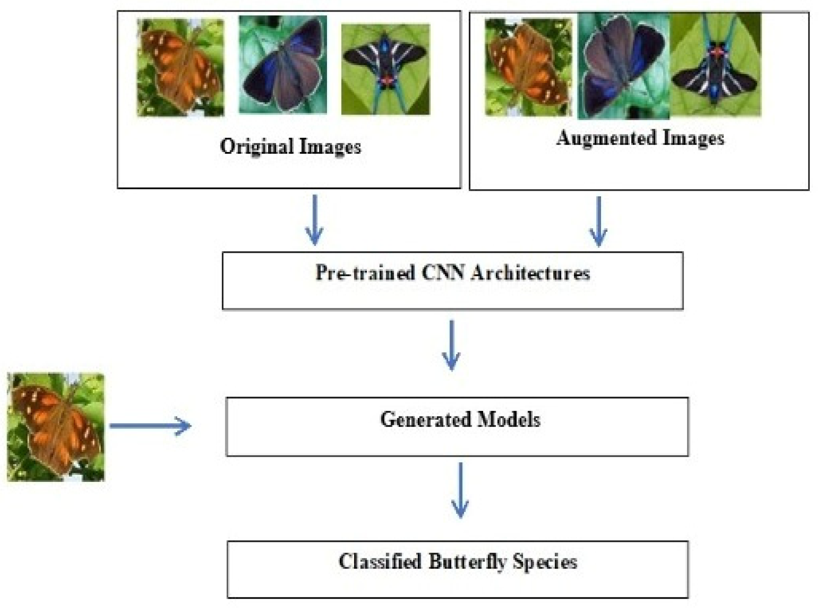
• Apply the data augmentation technique in order to obtain various combinations of original butterfly species.
• Apply the transfer learning technique to detect the type of the butterfly species without harming them physically. These augmented, i.e., transformed, data that are applied to various pre-trained CNN models help to improve the accuracy.

The rest of the paper is organized as follows: The literature overview of recent studies on butterfly species identification is discussed in Section 2. The data sets utilized, data augmentation techniques, and different state-of-the-art CNN-based transfer-learning models for butterfly species classification are discussed in Section 3. The performance evaluation of various classifiers is discussed in Section 4. The conclusion, as well as the future scope, is presented in Section 5.

2. Related Works

Zhu et al. [39] classified lepidopteran insect images, an integrative region matched, and the dual-complex discrete wavelet approach was presented. They tested their method on a collection of 100+ lepidopterous insects from 18 genera, and the recognition accuracy was found to be 84.47%. Silva et al. [40] wanted to see which feature selection strategies and classifiers were best for identifying honeybee subspecies among the seven feature pickers and classification methods available. In their experiments, they discovered that the best combination was the naive Bayes classifier and the mutual information extraction of features.

Wen et al. [41] incorporated local and global information for insect classification; researchers developed a model that incorporates K nearest neighbor classification (KNNC), regular densities predicated sequential classification model (NDLC), minimal level fewest linear classification algorithm (MLSLC), the nearest mean classifier (NMC), and decision tree (DT). Their experimental results showed an 86.6% classification rate when assessed on images taken during actual field trapping for training.

Kaya et al. [42] proposed two different local binary patterns (LPB) descriptors for detecting special textures in images. The first is based on the distance between the sequential neighbors of a center pixel. In contrast, the second is based on the central pixel parameter determining the neighbors in the same orientation. They used laboratory-based photos of 140 morphos obtained in Van, Turkey to evaluate their descriptors for identifying butterfly species. The artificial neural network has the greatest accuracy of 90.71% in classifying butterflies.

Faithpraise et al. [43] extracted structural information and used ANN to construct an automatic detection algorithm for copepod species. They assessed an overall accuracy of 93.13 % using seven copepod traits from 240 reference photos. Xie et al. [44] used advanced multiple-task sparse representation and multiple-kernel learning approaches; additional efforts were towards a classification method to categorize butterfly imagery. They applied the conceptual approach to the trial on 24 prevalent farming systems species and contrasted it to some newer approaches.

Feng et al. [45], relying on flap features of butterfly photos, improved an insect species recognition and retrieving method. Their recovery method is built upon the CBIR framework, which also does not require a formal confirmation but provides users with a range of matches. Abeysinghe et al. [46] used multilayer Siamese networks to build a completely computerized system for identifying snake species. Even though the original snake dataset is limited, they could attain consistent results. Alsing et al. [47] created genuine CNN infrastructure based on domain adaptation to detect post-it locations and then converted these algorithms to be used on smartphones and tablets. The fastest RCNN ResNet50 structure had the highest MAP (mean average precision) of 99.33%, but it took 20,018 milliseconds to infer.

Hernandez et al. [48] used a computational approach to categorize 740 species and 11,198 samples in a dataset. They were 91.65% accurate with fish, 92.87% with flora, and 91.25 % for butterflies. Iamsaata et al. [49] used the extreme learning machines (ELM) to categorize the butterflies and compare these results to the SVM algorithm. The ELM approach has a 90.37% accuracy, which is somewhat higher than the support vector machine (SVM).

Kang et al. [50] produced a unique neural network to classify butterflies based on the shape of their wings, with an accuracy of 80.3%. Bouzalmat et al. [51] used PCA and SVM to analyze two feature collections, the ATT and IFD datasets, which achieved 90.24 % and 66.8% accuracy. The literature survey identified that all models applied to butterfly species classification obtained 91.25%.

The above literature survey helps to understand that various machine-learning and deep-learning models are used to identify the butterfly species type. At present, pre-trained CNN models are very much used in classification and produce better accuracy also. The goal of this research work is to apply these pre-trained CNN models for the classification of butterfly species to improve the accuracy of machine-learning and deep-learning models. In addition to that, the proposed work adopts the data augmentation technique to produce a large dataset which will be helpful to predict the butterfly species correctly. A detailed description of data augmentation is discussed in Section 3.

3. Proposed System Methodology

Transfer-learning models, particularly convolutional neural networks, have performed well on image classification tasks. However, these models rely on a large dataset to produce accurate results and to avoid overfitting. The proposed work classifies butterfly species images into various classes using pre-trained transfer-learning models.

3.1. Dataset Description

To carry out this research work, the data set consists of 15 species of butterfly images, 1761 training images, 75 testing images of each fifteen classes, and 75 validation images of each fifteen classes chosen from Kaggle. All images were reduced to 350 × 350 pixels because they were of various resolutions. The input images include various features, such as occlusion and backdrop complexity, because they were captured with wide field-of-view cameras.

Table 1. Dataset Description.

Genus	Training Dataset	Testing Dataset	Validation Dataset
Africangaint Swallowtail	107	75	75
American Snoot	119	75	75
Atala	143	75	75
Banded Peacock	116	75	75
Becker’s White	105	75	75
Bkue Morphs	138	75	75
Crescent	108	75	75
Eastern Coma	133	75	75
Large Marble	112	75	75
Metamark	116	75	75
Painted Lady	116	75	75
Purple Hairstreak	107	75	75
Silver Spot Skipper	113	75	75
Tropical Leawing	119	75	75
Yellow Swallow Tail	118	75	75
Total	1761	1125	1125

lists the name and number of shots in the dataset for each butterfly genus.

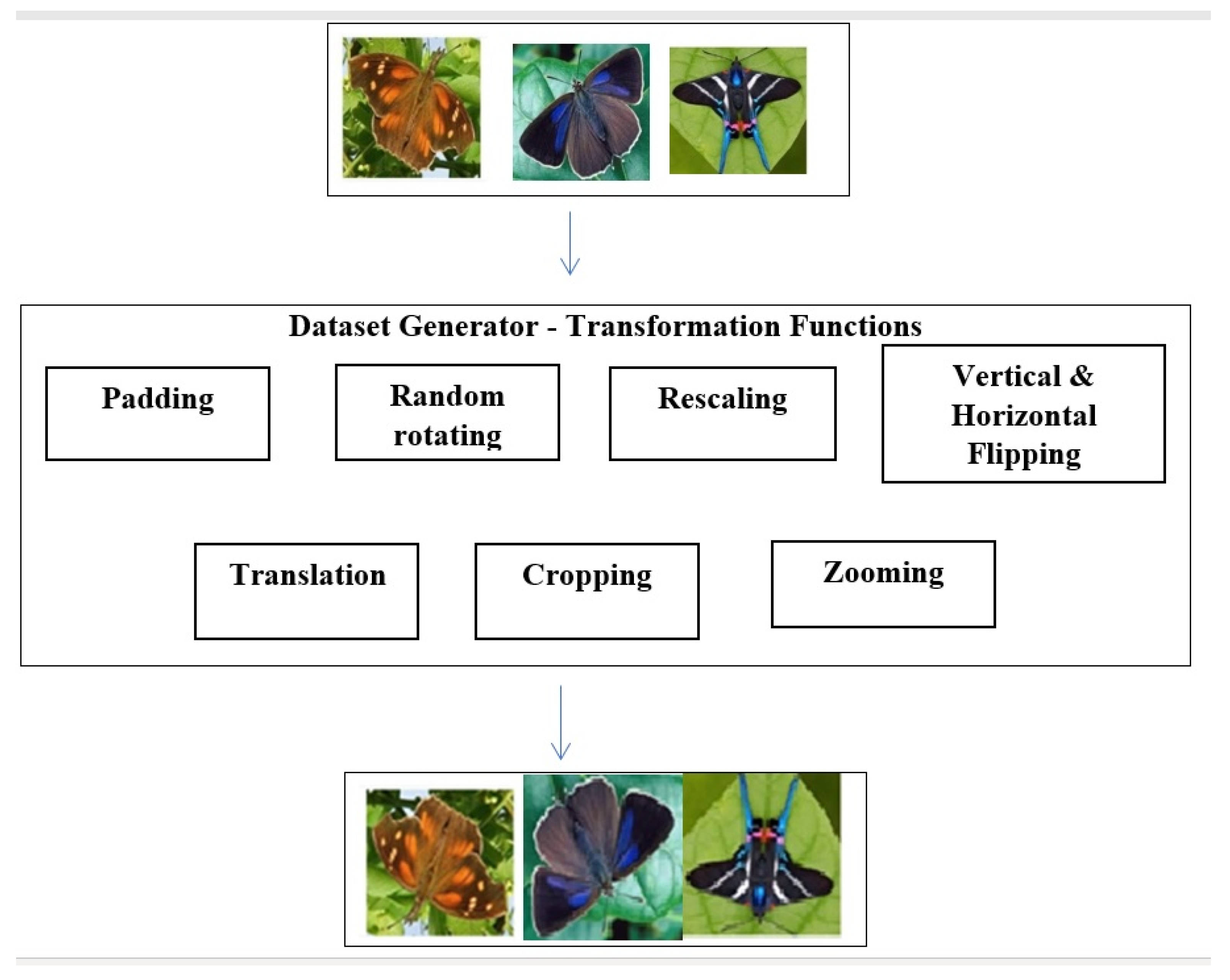
3.2. Data Augmentation

Data augmentation enhances the size and quality of training datasets. In the proposed model, all the original images are transformed by applying various transformation functions in each epoch using the Image Data Generator from the Keras framework. The newly generated images have different variations of the same image and are applied to transfer-learning models. Figure 1 represents the data augmentation process applied to the butterfly species dataset. The butterfly species image dataset containing the original batch of images is fed into the Image Data Generator image augmentation object, which produces a randomly transformed batch of images.

3.2.1. Cropping

Cropping is the process of positioning and squaring the entire image at a random location. A parameter determines the diagonal relative position just on image pixels. The square will be the same size as the picture if the value is 0, with no cropping. If the crop square is 50%, it will crop half of the source images in horizontal and vertical directions.

3.2.2. Rescaling

A layer that rescales input data to a new range as part of the pre-processing process. This layer rescales every input value (typically an image) by multiplying by the scale and adding an offset. The size of it varies based on the range. The squares will be the same dimension as the input if the scale is reduced to 0. The square will be in a randomized region around half the dimension and height and width of the object if the percentage is set to 50%.

3.2.3. Horizontal Flips

The horizontal flip argument specifies a Boolean value that flips the images horizontally. True causes them to be horizontally flipped. The vertical flip argument specifies a Boolean value that flips the images vertically.

3.2.4. Fill Mode

When you rotate an image, some pixels will move outside of the image, leaving an empty region that needs to be filled in. The default value for the fill mode option is “nearest,” which simply replaces the empty region with the closest pixel values.

3.2.5. Shear Range

Shear range = 0.2 says that the image will be sheared by 20%. Zoom range denotes a 20 % zoom-in and zoom-out range. Horizontal flip = True is set for mirror reflection. Fill mode is the most significant argument of Image Data Generator. There is some room left behind after the image shifts by 20%.

3.2.6. Width Shift

The width shift range is a floating-point value between 0.0 and 1.0 that determines the absolute limit of the fraction of the overall breadth. The image will be relocated to the left or right at irregular intervals.

3.2.7. Height Shift

It works the same as width_shift_range but shifts vertically (up or down).

3.2.8. Rotation Range

By passing an integer number in the rotation range argument to the Image Data Generator class, you can rotate images arbitrarily between 0 and 360 degrees. Some pixels will migrate outside the image as it is rotated, leaving an empty region that must be filled in.

3.3. Transfer-Learning Models

Transfer learning has risen to prominence as a crucial study area for artificial intelligence applications in recent years. Every day, the usage rate rises due to significant accomplishments in corresponding fields of speech recognition, computational linguistics, and human–computer interaction. Transfer-learning algorithms are based upon convolutional neural networks, influenced by the simplicity of synapses in a human mind. They have come to the forefront due to their effectiveness in learning. Transfer-learning methods can address the issue of feature extraction techniques by dynamically eliminating distinctive traits from the provided input data. Transfer learning requires a lot more labeled data than traditional neural networks. Transfer learning has become increasingly significant in problem solving because of the tremendous rise in available data. Many scientists in data analytics have noticed these remarks; CNNs are an upwards inter-feed-forward neural net regarding animal vision. A convolutional neural network is a deep-learning neural architecture used to classify images, discover similarities, and recognize objects. CNN, primarily employed for image classification, is now being used in practically every field where categorization is required. The basic convolutional neural architecture contains many numbers of numerous convolutions layers and maxpooling layers in succession, one to many fully linked parts, and finally, a classification output layer. Pre-trained transfer-learning neural prediction approaches such as VGG16, VGG19, MobileNet, Xception, ResNet50, and InceptionV3 are employed to classify the image. The proposed system workflow is represented in Figure 2.

3.3.1. VGG16

VGG16 is a CNN model developed by VGG at Oxford University. Alex Net, the channel’s replacement, emerged in 2012. VGG16 has eight levels, three fully associated layers, seven max-pooling layers upon layer, and one SoftMax layer. As part of the ImageNet contest, the architecture has been designed. The convolution blocks’ width is set to a tiny number. The width parameter is extended by two after each max-pooling operation until it reaches 512. The VGG16 has an image size of 224 × 224 pixels. Spatial cushioning was used to maintain the picture’s pixel density. The VGG16 network, which has been declared accessible, can be used to do similar functionality. The modeling can be leveraged for transfer learning in certain systems, such as Keras. These supply pre-trained weights can generate custom models with modest adjustments and produce higher accuracy.

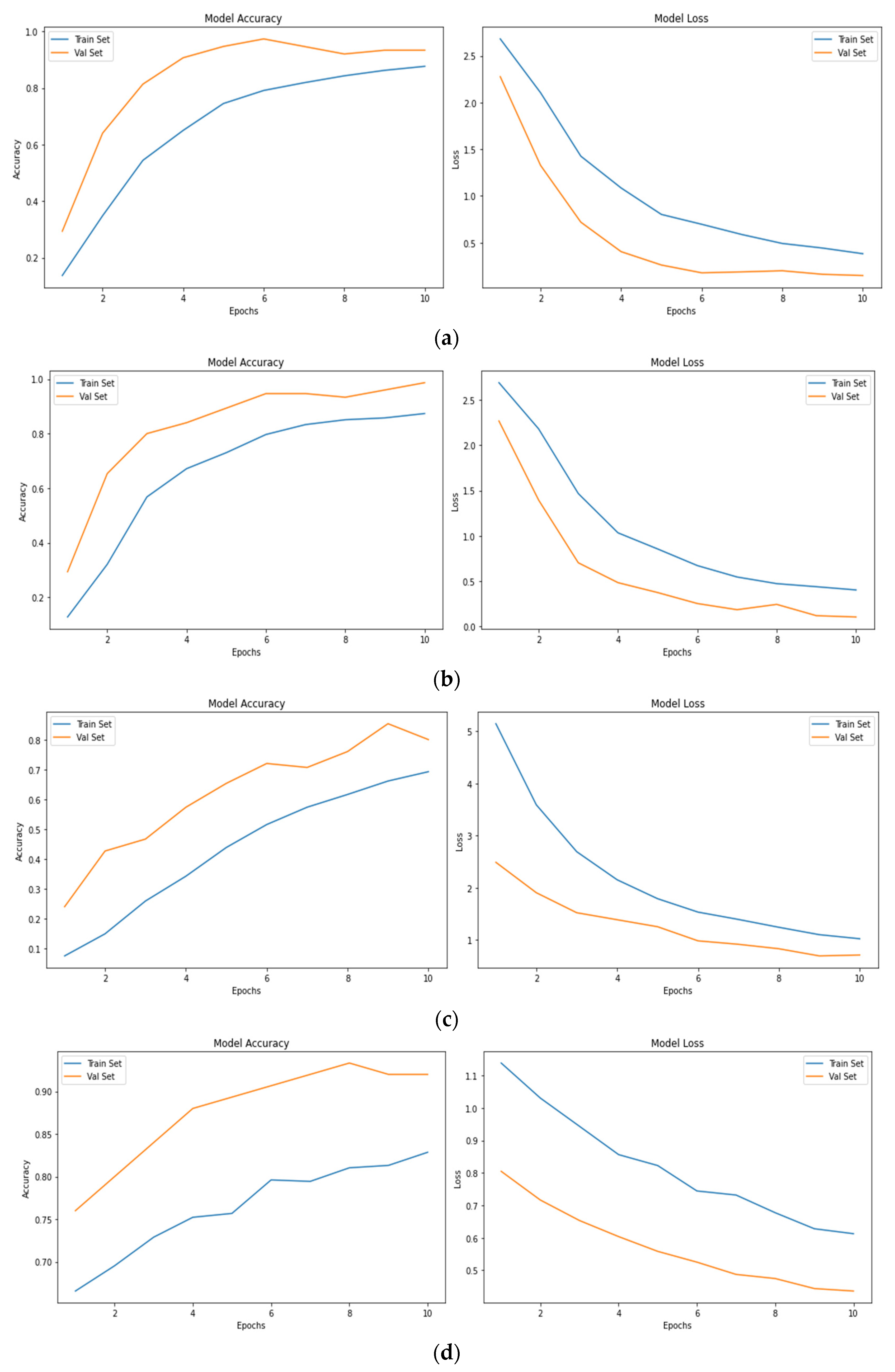
VGG16 without Data Augmentation

The input shape of the image is 350 × 350 pixels. The trainable layer in the base model is set as false, the model is sequential, and the activation function is sigmoid. The optimizer used in SGD has a learning rate of 0.0001 and the loss is categorical cross entropy. It has been validated for ten epochs. For input layer_2, the output shape is (None, 350, 350, 3) and the parameter is 0. For inblock1_conv1 layer, the output shape is (None, 350, 350, 64). The parameter 1792 is connected to the block2_conv2 where the output shape is (None, 350, 350, 64) and the parameter 36,928 is connected to the max-pooling layer where the output shape is (None, 350, 250, 64) and the parameter is 0. The same follows until block5 layer and the global_max_pooling layer where the output shape is (None, 10, 10, 512) and the parameter is 0. The flatten layer has output shape of (None, 51,200) and the parameter is 0. For the dense layer, the output shape is (None, 1024) and the parameter is 52,429,824 which is connected to the dropout layer where the output shape is (None, 1024) and the parameter is 0, which is connected to the dense layer which has the output shape of (None, 15) and the parameter of 15,375. The total number of parameters is 67,159,887 and the trainable parameters is 67,159,887 and the total non-trainable parameters is 0. The model has been trained for 10 epochs. In epoch 1, the loss value is 2.8380 and the value accuracy is 0.1411; in epoch2, the loss value is 2.1099 and the value accuracy is 0.3195, followed by an increase in the value accuracy and decrease in the value loss. In the 10th epoch, the loss is 0.0334 and the value accuracy is 0.9903. Thus, the model VGG16 without data augmentation has achieved the accuracy of 85.33%.

VGG16 with Data Augmentation

ImageDataGenerator is used for image pre-processing. The values for the parameters are rescale = 1.0/255.0, horizontal flip = True, fill mode = ‘nearest’, zoom range = 0.2, shear range = 0.2, width_shift_range = 0.2, height_shift_range = 0.2, and the rotation angle is 0.2. The batch size is 5, and the class mode is categorical. The input shape of the image is 350 × 350 pixels, and the pooling layer is the max-pooling layer. The model is the sequential model, and the activation function is sigmoid, the optimizer used in SGD with the learning rate of 0.0001, and the loss is categorical cross entropy. It has been validated for ten epochs. In epoch one the loss value is 2.6083, and the value accuracy is 0.1367. In epoch2, the loss value is 2.1047, and the value accuracy is 0.3749 followed by increase in the value accuracy and decrease in the value loss. In the 10th epoch, the loss is 0.3815, and the value accuracy is 0.8764. Thus, the model VGG16 with data augmentation has achieved an accuracy of 86.99%, and the loss value is 0.5347.

3.3.2. VGG19

VGG19 is a neural network trained on over a billion images in ImageNet. A laptop, keyboard, pencils, and a range of creatures are among the 1000 object classes the 19-layer network can classify photos into. As a result, the system has amassed a library of rich feature descriptions for a wide series of frames. VGGNet is architecture that stacks convolutional layers with tiny 33 receptive fields in blocks before adding a max-pooling layer. They use 11 convolutions in one network configuration to boost the nonlinearity of the decision function without modifying the convolutional layers’ receptive fields. We use the VGG19 design, which includes 19 weight layers, in this study.

VGG19 without Data Augmentation

The input shape of the image is 350 × 350 pixels. The num_class is 15, and the dropout layer is 0.25; it uses sigmoid as an activation function. The optimizer used is Adam, with a learning rate of 0.0001. The loss is categorical cross entropy, where the trainable layer is set as false the input layer_2, where the output shape is (None, 350, 350, 3) and the parameter is 0. In block1_ conv1 layer, the output shape is (None, 350, 350, 64). The parameter 1792 is connected to the block2_conv2 where the output shape is (None, 350, 350, 64) and the parameter is 36,928, connected to the max-pooling layer where the output shape is (None, 350, 250, 64) and the parameter is 0. The same follows until block5 layer and the global_max_pooling layer where the output shape is (None,10, 10, 512) and the parameter is 0. The flatten layer has output shape of (None, 51, 200) and the parameter is 0. In the dense layer, the output shape is (None, 1024) and the parameter is 52,429,824 which is connected to the dropout layer the output shape is (None, 1024) and the parameter is 0 which is connected to the dense layer which has the output shape of (None, 15) and the parameter of 15,375. The total number of parameters is 72,469,583. It has been validated for 10 epochs. In epoch 1, the loss value is 2.5518 and the value accuracy is 0.2323; in epoch2, the loss value is 1.0219 and the value accuracy is 0.6720 followed by increase in the value accuracy and decrease in the value loss. In the 10th epoch, the loss is 0.0088 and the value accuracy is 0.9994. Thus, the model VGG19 without data augmentation has achieved the accuracy of 90.66%.

VGG19 with Data Augmentation

ImageDataGenerator is used for image pre-processing. The values for the parameters are rescale = 1.0/255.0, horizontal_flip = True, fill_mode = ‘nearest’, zoom_range = 0.2, shear_range = 0.2, width_shift_range = 0.2, height_shift_range = 0.2, and the rotation angle is 0.2. The batch size is 5 and the class mode is categorical. The input shape of the image is 350 × 350 pixels, it used relu as activation function, and the dropout is 0.2. The final sigmoid layer with 4 nodes for classification output uses sigmoid as activation function. The optimizer used is RMSprop with the learning rate of 0.0001 and the loss is categorical cross entropy. It has been validated for 10 epochs. In epoch 1, the loss value is 2.6922 and the value accuracy is 0.1276; in epoch2 the loss value is 2.1818 and the value accuracy is 0.3206, followed by increase in the value accuracy and decrease in the value loss. In the 10th epoch, the loss is 0.4017 and the value accuracy is 0.8736. Thus, the model VGG19 with data augmentation has achieved the accuracy of 92.00% and the loss value is 0.3694.

3.3.3. MOBILENET

MobileNet employs depth-wise differentiated convolution layer. The set of parameters is significantly reduced when compared to a system using normal convolution layers of same depth in the networks. Light weighted deep-learning neural networks are constructed as a result. MobileNets are built using depth-wise separable convolution layers. Every insight-detachable convolutional layer is composed of a depth-wise convolution as well as a pointwise fully connected layer. A standard MobileNet’s number of parameters can be reduced to 4.2 million by adjusting the width multiplier hyperparameter. The size of the input image is 350 × 350 pixels.

MobileNet without Data Augmentation

The input shape of the image is 350 × 350 pixels. The trainable layer in base model is set as false, the model is sequential and the activation function is sigmoid. SGD is employed as the optimizer, with a detection rate of 0.0001 and a loss of categorical crossing entropy. In input layer_2, the output shape is (None, 350, 350, 3) and the parameter is 0. In conv1 layer, the output shape is (None, 175, 175, 32) and the parameter is 864, which connected to the batch normalization layer where the output shape is (None, 175, 175, 32) and the parameter is 128, which is connected to the relu layer where the output shape is (None, 175, 175, 32) and the parameter is 0. In depth-wise layer, the output shape is (None, 175, 175, 32) and the parameter is 288, which is connected to the batch normalization layer. It is followed as same for 13 relu functions. The flatten layer has output shape of (None, 165888) and the parameter is 0 which is connected to the mixed_10; in the dense, the output shape is (None, 1024) and the parameter shape is 1,049,600, which is connected to the flatten layer; in the dropout layer, the output shape is (None, 1024) and the parameter is 0 which is connected to the dense layer, which has the output shape (None, 15) and the parameter is 15,375, which is connected to the dropout layer. The total number of parameters is 4,293,839 and the trainable parameters are 4271.951 and the total non-trainable parameters are 21,888. It has been validated for 10 epochs. In epoch 1, the loss value is 5.1287 and the value accuracy is 0.0860; in epoch2, the loss value is 3.5716 and the value accuracy is 0.1350, followed by increase in the value accuracy and decrease in the value loss. In the 10th epoch, the loss is 1.3671 and the value accuracy is 0.5774. Thus, the model MobileNet with data augmentation has achieved the accuracy of 75.99% and the loss value of 0.7950.

MobileNet with Data Augmentation

Image Data Generator is used for image pre-processing. The values for the parameters are rescale = 1.0/255.0, horizontal_flip = True, fill_mode = ‘nearest’, zoom_range = 0.2, shear_range = 0.2, width_shift_range = 0.2, height_shift_range = 0.2, and the rotation angle is 0.2. The batch size is 5 and the class mode is categorical. The input shape of the image is 350 × 350 pixels. The trainable layer in base model is set as false, the model is sequential and the activation function is sigmoid. The optimizer used is SGD with the learning rate of 0.0001 and the loss is categorical cross entropy. It has been validated for 10 epochs. In epoch 1, the loss value is 5.1428 and the value accuracy is 0.0742; in epoch2, the loss value is 3.5890 and the value accuracy is 0.1492, followed by increase in the value accuracy and decrease in the value loss. In the 10th epoch, the loss is 1.0231 and the value accuracy is 0.6925. Thus, the model MobileNet with data augmentation has achieved an accuracy of 81.33% and the loss value is 0.8082.

3.3.4. XCEPTION

The Inception network has been phased out in favor of the Xception network. Xception is a term used to describe extreme inception. The Xception architecture employs larger values with separate convolutional parts rather than traditional fully connected layers. Xception accesses various spatial and bridge correlations, which in CNN-extracted features can be entirely disconnected. Inception’s basic architecture has been preserved a little longer than Xception, about 36, whereas convolution in the Xception architecture could be broken into 14 possible paths. After the initial and last levels are removed, every level has a persistent remnant link surrounding it. The incoming image is converted to identify the likelihood in each output of acquiring cross-channel similarities. The depth-wise 11 convolution approach is then applied. Rather than 3D mappings, the interconnections can be represented as a 2D + 1D mapping. Inception commences with a 2D area connection, which 1D space correlations would precede.

Xception without Data Augmentation

The input shape of the image is 350 × 350 pixels. The trainable layer in base model is set as false, the model is sequential and the activation function is sigmoid. The optimizer used is SGD with the learning rate of 0.0001 and the loss is categorical cross entropy. It has been validated for 10 epochs. In the input layer_1, the output shape is (None, 350, 350, 3) and the parameter is 0. In the conv1 layer, the output shape is (None, 175, 175, 32), and the parameter is 864 is connected to the input_layer1 where the output shape is (None, 175, 175, 32) and the parameter is 128, which is connected to the activation layer where the output shape is (None, 175, 175, 32) and the parameter is 0. In the depth-wise layer, the output shape is (None, 175, 175, 32), and the parameter is 0, which is connected to the batch normalization layer. The same follows until block14 layer and the global_max_pooling layer where the output shape is (None, 2048) and the parameter is 0, which is connected to the block14. The flatten layer has an output shape of (None, 2048), and the parameter is 0, which is connected to the global max-pooling layer; in the dense layer, the output shape is (None, 1024) and the parameter shape is 2,098,176 which is connected to the flatten layer; in the dropout layer, the output shape is (None, 1024) and the parameter is 0 which is connected to the dense layer; finally, in the dense layer, the output shape is (None, 15) and the parameter is 15,375 which is connected to the dropout layer. The total number of parameters is 22,975,031, the trainable parameters is 22,920,503, and the total non-trainable parameters is 54,528. In epoch 1, the loss value is 1.1388 and the value accuracy is 0.6657; in epoch2, the loss value is 1.0308 and the value accuracy is 0.6953 followed by increase in the value accuracy and decrease in the value loss. In the 10th epoch, the loss is 0.6127, and the value accuracy is 0.8286. Thus, the model Xception without data augmentation has achieved an accuracy of 87.99%.

Xception with Data Augmentation

ImageDataGenerator is used for image pre-processing. The values for the parameters are rescale = 1.0/255.0, horizontal_flip = True, fill_mode = ‘nearest’, zoom_range = 0.2, shear_range = 0.2, width_shift_range = 0.2, height_shift_range = 0.2, and the rotation angle is 0.2. The batch size is 5 and the class mode is categorical. The input shape of the image is 350 × 350 pixels; the pooling layer is max-pooling layer. The model is sequential models and the activation function is sigmoid; the optimizer used is SGD with the learning rate of 0.0001 and the loss is categorical cross entropy. It has been validated for 10 epochs. In epoch 1, the loss value is 1.1388 and the value accuracy is 0.9957; in epoch2, the loss value is 1.0308 and the value accuracy is 0.6953 followed by increase in the value accuracy and decrease in the value loss. In the 10th epoch, the loss is 0.6127 and the value accuracy is 0. 8286. Thus, the model Xception with data augmentation has achieved an accuracy of 87.99%.

3.3.5. RESNET50

ResNet differs from other standard subsequent communication networks, including VGGNet and Alex Net, because it has segments and sub-module structures different from other architectures. It may be preferable to shift to the lower layer and ignore the level transitions. ResNet’s architecture addresses this situation, and the network’s success rate improves by reducing the challenge of recalling the system. ResNet is a 177-layer neural network. There is information on how multi-interconnections will be established in conjunction with the large-scale project. This model has been trained on photos with a size of 224 × 224 × 3.

Resnet50 without Data Augmentation

The input shape of the image is 350 × 350 pixels. It uses a sigmoid as an activation function. The optimizer used is SGD with the learning rate of 0.0001 and the loss is categorical cross entropy, where the trainable layer is set as false. In input layer_2, the output shape is (None, 350, 350, 3) and the parameter is 0. In conv1_pad layer, the output shape is (None, 350, 350, 3) and the parameter is 0 which is connected to the input1 layer, where the output shape is (None, 350, 350, 64) and the parameter is 9427, which is connected to the batch normalization layer where the output shape is (None, 175, 175, 64) and the parameter 256, which is connected to the conv1 layer. The same follows until block5 layer and the global_max_pooling where layer the output shape is (None, 2048) and the parameter is 0. The flatten layer has output shape of (None, 2048) and the parameter is 0. In the dense layer, the output shape is (None, 1024) and the parameter is 209,8176, which is connected to the dropout layer where the output shape is (None, 1024) and the parameter is 0, which is connected to the flatten layer which has the output shape of (None, 1024) and the parameter is 15,375. The total number of parameters is 25,701,263, the non-trainable parameter is 2,113,551 and the non-trainable parameters is 23,587,712. It has been validated for 10 epochs. In epoch 1, the loss value is 3.7351 and the value accuracy is 0.0746; in epoch2, the loss value is 3.2707 and the value accuracy is 0.0866 followed by increase in the value accuracy and decrease in the value loss. In the 10th epoch, the loss is 2.2222 and the value accuracy is 0.2882. Thus, the model ResNet50 with data augmentation has achieved an accuracy of 38.66%.

Resnet50 with Data Augmentation

ImageDataGenerator is used for image pre-processing. The values for the parameters are rescale = 1.0/255.0, horizontal_flip = True, fill_mode = ‘nearest’, zoom_range = 0.2, shear_range = 0.2, width_shift_range = 0.2, height_shift_range = 0.2, and the rotation angle is 0.2. The batch size is 5 and the class mode is categorical. The input shape of the image is 350 × 350 pixels. The trainable layer in base model is set as false, the model is sequential and the activation function is sigmoid. The optimizer used is SGD with the learning rate of 0.0001 and the loss is categorical cross entropy. It has been validated for 10 epochs. In epoch 1, the loss value is 3.4661 and the value accuracy is 0.1071; in epoch2, the loss value is 2.6349 and the value accuracy is 0.1726, followed by increase in the value accuracy and decrease in the value loss. In the 10th epoch, the loss is 2.1626 and the value accuracy is 0.3013. Thus, the model Xception with data augmentation has achieved an accuracy of 43.99%.

3.3.6. INCEPTIONV3

Inception is an add-on to the Xception architecture that uses a complexity-separated convolution layer instead of the standard convolution layers. The Inception model is a neural network that helps classify objects in images. Another term for Inception is Google Net. During the training phase, the ImageNet dataset is utilized. The photographs for Inception must have a resolution of 299 × 299 × 3. By lowering dimensions with a layered 11 convolution layer, Inception convolutional neural networks can deliver more effective computing and deep connections. The components were developed to address issues such as computation complexity and generalization, among many others.

InceptionV3 without Data Augmentation

The input shape of the image is 350 × 350 pixels; it used relu as an activation function and the dropout is 0.2. The final sigmoid layer with 4 nodes for classification output uses sigmoid as an activation function. The optimizer used is RMSprop with the learning rate of 0.0001 and the loss is categorical cross entropy. In input layer1, output shape is (None, 350, 350, 3) and the parameter is 0. In conv2d layer, the output shape is (None, 174, 174, 32, 864) and the parameter is 0, which is connected to the input1. In the batch normalization layer, the output shape is (None, 174, 174, 32, 96) and the parameter is 96 which is connected to the output layer of conv2d. In activation layer, the output shape is (None, 174, 174, 32, 0) and the parameter is 0, which is connected to the batch normalization layer, and in conv2d_1 layer the output shape is (None, 172,172, 32, 9216) and the parameter is 96; this is connected to the output layer of batch normalization layer 1. This is followed by the activation function of 93 where the output shape is (None, 9, 9, 192) and the parameter is 0 which is connected to the (activation_85, mixed9_1, concatenate_1 and activation_93); the flatten layer has output shape of (None, 165888). The parameter is 0 which is connected to the mixed_10; in the dense layer, the output shape is (None, 1024) and the parameter shape is 169,870,336 which is connected to the flatten layer; in the dropout layer, the output shape is (None, 1024) and the parameter is 0, which is connected to the dense layer which has the output shape of (None, 15). The parameter 15,375 is connected to the dropout layer. The total number of parameters is 191,688,495, trainable parameters is 169,885,711 and the total non-trainable parameters is 21,802,784. It has been validated for 10 epochs. In epoch 1, the loss value is 117.8563 and the value accuracy is 0.2437; in epoch2, the loss value is 4.8096 and the value accuracy is 0.2688 followed by increase in the value accuracy and decrease in the value loss. In the 10th epoch, the loss is 2.2486 and the value accuracy is 0.4243. Thus, the model inception without data augmentation has achieved the accuracy of 42.66%.

InceptionV3 with Data Augmentation

ImageDataGenerator is used for image pre-processing. The values for the parameters are rescale = 1.0/255.0, horizontal_flip = True, fill_mode = ‘nearest’, zoom_range = 0.2, shear_range = 0.2, width_shift_range = 0.2, height_shift_range = 0.2, and the rotation angle is 0.2. The batch size is 5 and the class mode is categorical. The input shape of the image is 350 × 350 pixels, it used relu as an activation function and the dropout is 0.2. The final sigmoid layer with 4 nodes for classification output uses sigmoid as an activation function. The optimizer used is RMSprop with the learning rate of 0.0001 and the loss is categorical cross entropy. It has been validated for 10 epochs. In epoch 1, the loss value is 3.0758 and the value accuracy is 0.5011; in epoch2, the loss value is 1.1765 and the value accuracy is 0.7187 followed by increase in the value accuracy and decrease in the value loss. In the 10th epoch, the loss is 0.4305 and the value accuracy is 0.9060. Thus, the model Inception with data augmentation has achieved an accuracy of 94.66%, and the loss is 0.8228.

4. Performance Evaluation

Each and every model has a model parameter that is internal to the specific model and its value is estimated from the given data. To improve the performance of the models, we can tune the parameters such as epochs, learning rate, etc., of each pre-trained model, and the detailed explanation about parameter tuning is mentioned in Section 3.3.1, Section 3.3.2, Section 3.3.3, Section 3.3.4, Section 3.3.5 and Section 3.3.6. Certain activation functions are employed to lessen the nonlinearity in a neuron’s output. The output’s gradient-activating function determines the kind of forecasts the system can generate. For all of the models in the present scheme, the Softmax layer is used as the activation function. The network output, SoftMax, is utilized in the deep network to forecast a multinomial probability distribution. The “loss” is the network’s prediction error, while the “loss function” is the process for computing it. The loss function also calculates the gradients. The weights of the neural network are updated using gradients. Categorical cross entropy were used to multi-task the classification tasks. It can be any possible category, and the model should decide the best among the ones. Image augmentation increases the amount of data used to train the network. The datasets are broken into three sections: training, validation, and testing datasets. Training is the collection of dataset samples used to learn how to adjust the input data to obtain the desired output. Validation is a set of dataset samples used to fine-tune the input dataset’s sample of a classifier. After training and validating the data for ten epochs, the class species of the images is calculated. The outcomes were determined by assessing performance indicators, loss, and value accuracy. The parameters such as batch size, image dimension, optimizer, activation function, and loss function used for the state-of-the-art CNN-based pre-trained transfer-learning models are represented in

Table 2. Parameters of CNN based pre-trained transfer-learning Models.

Performance Measures	VGG16	VGG19	MobileNet	Xception	ResNet50	Inception V3
Batch Size	5	5	5	5	5	5
Image Dimension	350 × 350	350 × 350	350 × 350	350 × 350	350 × 350	350 × 350
Optimizer	SGD	Adam	SGD	SGD	SGD	RMSprop
Activation Function	Sigmoid	Sigmoid	Sigmoid	Sigmoid	Sigmoid	Sigmoid
Loss Function	Categorical Cross entropy	Categorical Cross entropy	Categorical Cross entropy	Categorical Cross entropy	Categorical Cross entropy	Categorical Cross entropy

.

4.1. Accuracy and Loss Values of Pre-Trained Transfer Learning Models

Pre-trained CNN models such as VGG16, VGG19, MobileNet, Xception, and ResNet50 have far more hyperparameters in reality than InceptionV3. The Inception V3 model concentrates on the convolution operation of 3 × 3 filters in phase one and padding together with max-pooling layers of 2 × 2 filters in stride two, rather than having a bunch of hyperparameters. As a result, Inception V3′s classification performance is better at detecting the butterfly’s genus representations. All of the models’ accuracy and loss values are plotted against epochs from Figure 3a,f.

The accuracy value represents the performance of the model. In general, the loss value represents the sum of errors in the model. A good model should exhibit lower loss and higher accuracy. From Figure 3a,f, it is understood that the lowest loss and highest error are achieved in the Inception V3 model. This best accuracy is obtained due to label smoothing, 7 × 7 convolutions, and auxiliary classifier features of the Inception V3 model.

4.2. Accuracy of Pre-Trained Transfer Learning Models

Table 3. Accuracy of pre-trained CNN based transfer-learning Models.

Models	Without Data Augmentation	With Data Augmentation
InceptionV3	42.66	94.66
VGG19	90.66	92.00
Xception	81.33	87.99
VGG16	85.33	86.66
MobileNet	75.99	81.33
ResNet50	38.66	43.99

compares the performance of models that use data augmentation vs. models that do not use data augmentation. The results suggest that pre-trained transfer-learning CNN models perform better when identifying species of butterflies in imagery.

The InceptionV3 method uses a normal dense architecture to mimic a sparse CNN. Because only a few hidden neurons are required, the spacing of convolutional filters in a particular kernel size is reduced to a minimum. Convolution layers of varying sizes are also used to collect features from different scales. As a result, the InceptionV3 model is the best for attaining greater accuracy.

4.3. Precision, Recall, F1-Score of Inception V3 Model

The precision, recall, and F1-score of the Inception V3 model are shown in

Table 4. Precision, Recall, F1-Score of Inception V3 model with data augmentation.

Species Classes	Precision	Recall	F1-Score	Support
African Giant Swallowtail	1.00	1.00	1.00	5
American Snoot	0.83	1.00	0.91	5
Atala	1.00	1.00	1.00	5
Banded Peacock	0.83	1.00	0.91	5
Becker’s White	1.00	1.00	1.00	5
Blue Morpho	0.83	1.00	0.91	5
Crescent	1.00	0.80	0.89	5
Eastern Coma	1.00	1.00	1.00	5
Large Marble	1.00	1.00	1.00	5
Metalmark	1.00	1.00	1.00	5
Painted Lady	0.83	1.00	0.91	5
Purple Hairstreak	1.00	0.60	0.75	5
Silver Spot Skipper	1.00	1.00	1.00	5
Tropical Leafwing	1.00	0.80	0.89	5
Yellow Swallow Tail	1.00	1.00	1.00	5

. The result shows that the highest precision of 1 is obtained for 11 classes out of 15 classes, indicating that these 11 classes of butterfly species are predicted accurately. Similarly, 11 classes obtained the recall value of 1, meaning that most of the relevant images were retrieved. F1-score is the weighted average of precision and recall.

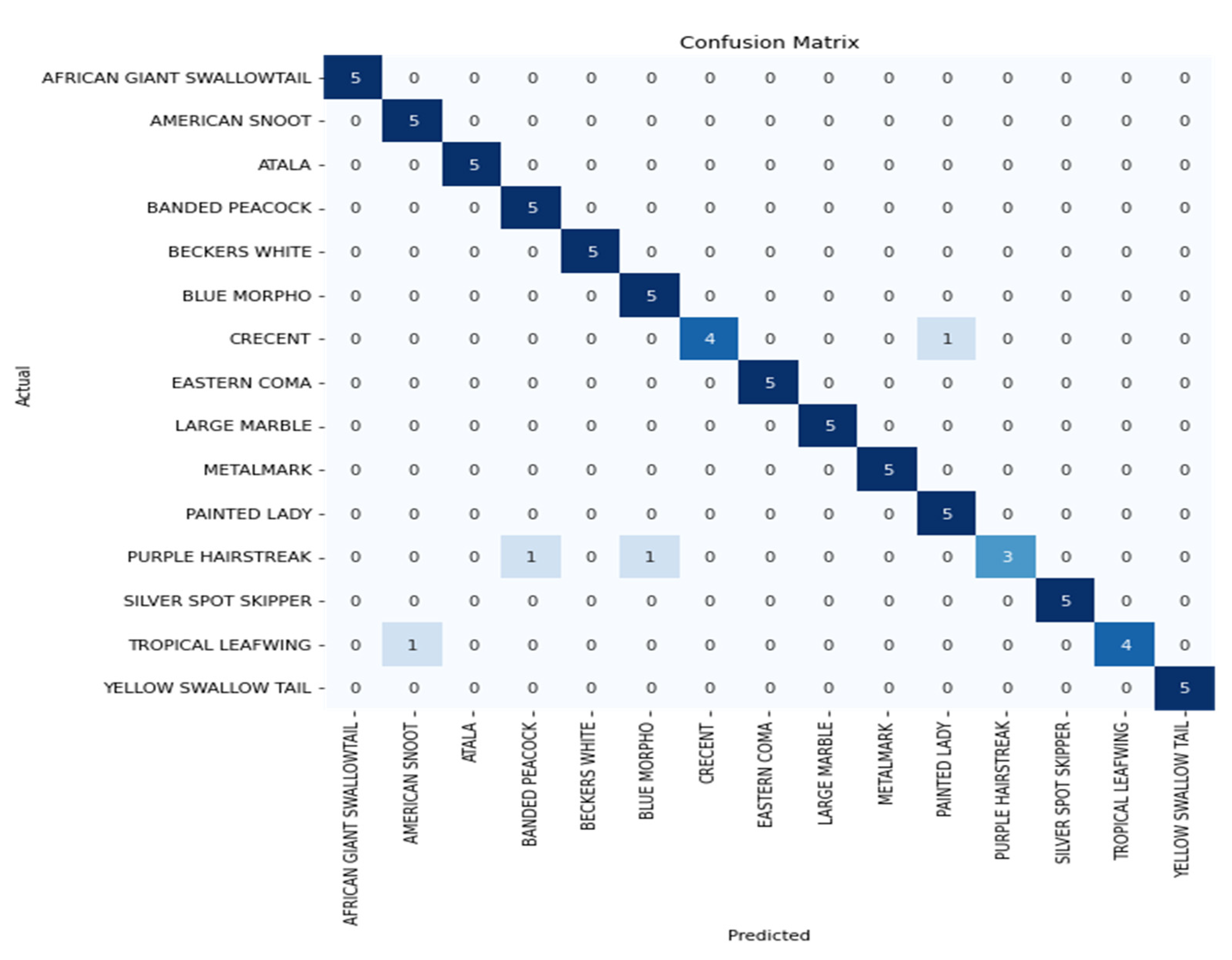
4.4. Confusion Matrix

The confusion matrix obtained by the Inception V3 model with data augmentation is shown in Figure 4. The result shows that out of 15 classes, 12 classes were correctly classified, whereas images in 3 classes such as a crescent, purple hairstreak, and tropical leafwing were wrongly classified by the Inception V3 model.

5. Conclusions and Future Scope

The proposed research work aimed to help science students to analyze butterfly species type without harming them by applying pre-trained CNN models. In order to achieve better accuracy, these pre-trained models require a large dataset which is prepared by applying data transformation techniques. The proposed system compares ubiquitous and effective pre-trained transfer-learning models for identifying the specific species of butterflies by analyzing butterfly species visuals. Data augmentation is used to gain more pictures because the species images collected by Kaggle are restricted. Transfer-learning algorithms are recommended to provide efficient results by identifying butterfly species. Pre-trained transfer-learning neural network models such as VGG16, VGG19, MobileNet, Xception, ResNet50, and Inception V3 are employed in this proposed work. The models categorize fifteen different species of butterflies, and their performance is validated using a test dataset, yielding anticipated efficiency for all of them. Performance indicators, including accuracy, precision, recall, and F1-score, assess the model’s performance. Out of all models, InceptionV3 with data augmentation has the highest accuracy of 94.64% among all the transfer learning models. The confusion matrix presented in Section 4.4 depicts that this model was able to predict 12 classes correctly out of 15 classes. This research work mainly concentrates on obtaining the best model to classify butterflies among all the pre-trained CNN models. However, the limitation lies in the fact that the data used for classification are purely images. This work can be further extended to obtain multiple input images from real-time videos taken which contain multimodal data, i.e., both images and sounds of species and then apply this multimodal data into pre-trained models. In future work, we are planning to increase the test sets to improve the accuracy of the evaluation results.

References

1. Fauzi, F.; Permanasari, A.E.; Setiawan, N.A. Butterfly Image Classification Using Convolutional Neural Net-work (CNN). In Proceedings of the 2021 3rd International Conference on Electronics Representation and Algorithm (ICERA), Yogyakarta, Indonesia, 29–30 July 2021; pp. 66–70. [Google Scholar]
2. Fan, L.; Zhou, W. An Improved Contour Feature Extraction Method for the Image Butterfly Specimen. In 3D Imaging Technologies—Multidimensional Signal Processing and Deep Learning; Springer: Singapore, 2021; pp. 17–26. [Google Scholar]
3. Ali, M.A.S.; Balasubramanian, K.; Krishnamoorthy, G.D.; Muthusamy, S.; Pandiyan, S.; Panchal, H.; Mann, S.; Thangaraj, K.; El-Attar, N.E.; Abualigah, L.; et al. Classification of Glaucoma Based on Elephant-Herding Optimization Algorithm and Deep Belief Network. Electronics 2022, 11, 1763. [Google Scholar] [CrossRef]
4. Chen, X.; Wang, B.; Gao, Y. Gaussian Convolution Angles: Invariant Vein and Texture Descriptors for Butterfly Species Identification. In Proceedings of the 2020 25th International Conference on Pattern Recognition (ICPR), Milan, Italy, 10–15 January 2021; pp. 5798–5803. [Google Scholar]
5. Min, F.; Xiong, W. Butterfly Image Generation and Recognition Based on Improved Generative Adversarial Networks. In Proceedings of the 2021 4th International Conference on Robotics, Control and Automation Engineering (RCAE), Wuhan, China, 4–6 November 2021; pp. 40–44. [Google Scholar] [CrossRef]
6. Xi, T.; Wang, J.; Han, Y.; Lin, C.; Ji, L. Multiple butterfly recognition based on deep residual learning and image analysis. Èntomol. Res. 2022, 52, 44–53. [Google Scholar] [CrossRef]
7. Houssein, E.H.; Abdelminaam, D.S.; Hassan, H.N.; Al-Sayed, M.M.; Nabil, E. A hybrid barnacles mating optimizer algorithm with support vector machines for gene selection of microarray cancer classification. IEEE Access 2021, 9, 64895–64905. [Google Scholar] [CrossRef]
8. Marta, S.; Luccioni, A.; Rolnick, D. Spatiotemporal Features Improve Fine-Grained Butterfly Image Classification. In Proceedings of the Conference on Neural Information Processing Systems; 2020. Available online: https://s3.us-east-1.amazonaws.com/climate-change-ai/papers/neurips2020/63/paper.pdf (accessed on 14 May 2022).
9. Houssein, E.H.; Hassaballah, M.; Ibrahim, I.E.; AbdElminaam, D.S.; Wazery, Y.M. An automatic arrhythmia classification model based on improved marine predators algorithm and convolutions neural networks. Expert Syst. Appl. 2022, 187, 115936. [Google Scholar] [CrossRef]
10. Almryad, A.; Kutucu, H. Automatic Detection of Butterflies by convolutional neural networks. Eng. Sci. Technol. Int. J. 2020, 23, 189–195. [Google Scholar]
11. Houssein, E.H.; Abdelminaam, D.S.; Ibrahim, I.E.; Hassaballah, M.; Wazery, Y.M. A hybrid heartbeats classification approach based on marine predators algorithm and convolution neural networks. IEEE Access 2021, 9, 86194–86206. [Google Scholar] [CrossRef]
12. Zhao, R.; Li, C.; Ye, S.; Fang, X. Deep-red fluorescence from isolated dimers: A highly bright excimer and imaging in vivo. Chem. Sci. 2001, 291, 213–225. [Google Scholar]
13. Nijhout, H.F. Elements of butterfly wing patterns. J. Exp. Zool. 2001, 291, 213–225. [Google Scholar] [CrossRef]
14. Pinzari, M.; Santonico, M.; Pennazza, G.; Martinelli, E.; Capuano, R.; Paolesse, R.; Di Rao, M.; D’Amico, A.; Cesaroni, D.; Sbordoni, V.; et al. Chemically mediated species recognition in two sympatric Grayling butterflies. PLoS ONE 2018, 13, e0199997. [Google Scholar] [CrossRef]
15. Austin, G.T.; Riley, T.J. Portable bait traps for the study of butterflies. Trop. Lepid. Res. 1995, 6, 5–9. [Google Scholar]
16. Ries, L.; Debinski, D.M.; Wieland, M.L. Conservation value of roadside prairie restoration to butterfly community. Conserv. Biol. 2001, 15, 401–411. [Google Scholar] [CrossRef]
17. Fina, F.; Birch, P.; Young, R.; Obu, J.; Faithpraise, B.; Chatwin, C. Automatic plant pest detection and recognition using k-means clustering algorithm and correspondence filters. Int. J. Adv. Biotechnol. Res. 2013, 4, 189–199. [Google Scholar]
18. Leow, L.K.; Chew Li Chong, V.C.; Dhillon, S.K. Automated identification of copepods using digital image processing and artificial neural network. BMC Bioinf. 2015, 16, S4. [Google Scholar] [CrossRef] [PubMed] [Green Version]
19. Mayo, M.; Watson, A.T. Automatic species identification of live moths. Knowl. Based Syst. 2007, 20, 195–202. [Google Scholar] [CrossRef] [Green Version]
20. Tan, A.; Zhou, G.; He, M. Rapid Fine-Grained Classification of Butterflies Based on FCM-KM and Mask R-CNN Fusion. IEEE Access 2020, 8, 124722–124733. [Google Scholar] [CrossRef]
21. Salama AbdELminaam, D.; Almansori, A.M.; Taha, M.; Badr, E. A deep facial recognition system using computational intelligent algorithms. PLoS ONE 2020, 15, e0242269. [Google Scholar] [CrossRef]
22. Kartika, D.S.Y.; Herumurti, D.; Rahmat, B.; Yuniarti, A.; Maulana, H.; Anggraeny, F.T. Combining of Extraction Butterfly Image using Color, Texture and Form Features. In Proceedings of the 6th Information Technology International Seminar (ITIS), Surabaya, Indonesia, 14–16 October 2020; pp. 98–102. [Google Scholar]
23. Rodrigues, R.; Manjesh, R.; Sindhura, P.; Hegde, S.N.; Sheethal, A. Butterfly species identification using convolutional neural network. Int. J. Res. Eng. Sci. Manag. 2020, 3, 245–246. [Google Scholar]
24. Theivaprakasham, H. Identification of Indian butterflies using Deep Convolutional Neural Network. J. Asia-Pacific Èntomol. 2021, 24, 329–340. [Google Scholar] [CrossRef]
25. Lin, Z.; Jia, J.; Gao, W.; Huang, F. Fine-grained visual categorization of butterfly specimens at sub-species level via a convolutional neural network with skip-connections. Neurocomputing 2020, 384, 295–313. [Google Scholar] [CrossRef]
26. Zhu, L.-Q.; Zhang, Z. Insect recognition based on integrated region matching and dual tree complex wavelet transform. J. Zhejiang Univ. Sci. C 2011, 12, 44–53. [Google Scholar] [CrossRef]
27. da Silva, F.L.; Sella, M.L.G.; Francoy, T.M.; Costa, A.H.R. Evaluating classification and feature selection techniques for honeybee subspecies identification using wing images. Comput. Electron. Agric. 2015, 114, 68–77. [Google Scholar] [CrossRef]
28. Wen, C.; Guyer, D. Image-based orchard insect automated identification and classification method. Comput. Electron. Agric. 2012, 89, 110–115. [Google Scholar] [CrossRef]
29. Kaya, Y.; Kaycı, L. Application of artificial neural network for automatic detection of butterfly species using color and texture features. Visual Comput. 2014, 30, 71–79. [Google Scholar] [CrossRef]
30. Xie, C.; Zhang, J.; Li, R.; Li, J.; Hong, P.; Xia, J.; Chen, P. Automatic classification for field crop insects via multiple-task sparse representation and multiple-kernel learning. Comput. Electron. Agric. 2015, 119, 123–132. [Google Scholar] [CrossRef]
31. Feng, L.; Bhanu, B.; Heraty, J. A software system for automated identification and retrieval of moth images based on wing attributes. Pattern Recognit. 2016, 51, 225–241. [Google Scholar] [CrossRef]
32. Abeysinghe, C.; Welivita, A.; Perera, I. Snake image classification using Siamese networks. In Proceedings of the 2019 3rd In-ternational Conference on Graphics and Signal Processing, Hong Kong, China, 1–3 June 2019; pp. 8–12. [Google Scholar] [CrossRef]
33. Alsing, O. Mobile Object Detection Using Tensorflow Lite and Transfer Learning. Master’s Thesis, KTH School of Electrical Engineering and Computer Science (EECS), Stockholm, Sweden, 2018. [Google Scholar]
34. Hernandez-Serna, A.; Jim’enez-Segura, L.F. Automatic identification of species with neural networks. PeerJ 2014, 2, e563. [Google Scholar] [CrossRef] [Green Version]
35. Iamsaata, S.; Horataa, P.; Sunata, K.; Thipayanga, N. Improving butterfly family classification using past separating features extraction in extreme learning machine. In Proceedings of the 2nd International Conference on Intelligent Systems and Image Processing; The Institute of Industrial Applications Engineers: Kitakyushu, Fukuoka, Japan, 2014. [Google Scholar]
36. Kang, S.-H.; Cho, J.-H.; Lee, S.-H. Identification of butterfly based on their shapes when viewed from different angles using an artificial neural network. J. Asia-Pacific Entomol. 2014, 17, 143–149. [Google Scholar] [CrossRef]
37. Bouzalmat, A.; Kharroubi, J.; Zarghili, A. Comparative Study of PCA, ICA, LDA using SVM Classifier. J. Emerg. Technol. Web Intell. 2014, 6, 64–68. [Google Scholar] [CrossRef] [Green Version]
38. Xin, D.; Chen, Y.-W.; Li, J. Fine-Grained Butterfly Classification in Ecological Images Using Squeeze-And-Excitation and Spatial Attention Modules. Appl. Sci. 2020, 10, 1681. [Google Scholar] [CrossRef] [Green Version]
39. Zhu, L.; Spachos, P. Towards Image Classification with Machine Learning Methodologies for Smartphones. Mach. Learn. Knowl. Extr. 2019, 1, 1039–1057. [Google Scholar] [CrossRef] [Green Version]
40. Rashid, M.; Khan, M.A.; Alhaisoni, M.; Wang, S.-H.; Naqvi, S.R.; Rehman, A.; Saba, T. A Sustainable Deep Learning Framework for Object Recognition Using Multi-Layers Deep Features Fusion and Selection. Sustainability 2020, 12, 5037. [Google Scholar] [CrossRef]
41. Alzubaidi, L.; Fadhel, M.; Al-Shamma, O.; Zhang, J.; Santamaría, J.; Duan, Y.; Oleiwi, S. Towards a Better Understanding of Transfer Learning for Medical Imaging: A Case Study. Appl. Sci. 2020, 10, 4523. [Google Scholar] [CrossRef]
42. Barbedo, J.G.A. Detecting and Classifying Pests in Crops Using Proximal Images and Machine Learning: A Review. AI 2020, 1, 312–328. [Google Scholar] [CrossRef]
43. Fang, X.; Jie, W.; Feng, T. An Industrial Micro-Defect Diagnosis System via Intelligent Segmentation Region. Sensors 2019, 19, 2636. [Google Scholar] [CrossRef] [Green Version]
44. Elminaam, D.S.A.; Neggaz, N.; Ahmed, I.A.; Abouelyazed, A.E.S. Swarming Behavior of Harris Hawks Optimizer for Arabic Opinion Mining. Comput. Mater. Contin. 2021, 69, 4129–4149. [Google Scholar] [CrossRef]
45. AbdElminaam, D.S.; Neggaz, N.; Gomaa, I.A.E.; Ismail, F.H.; Elsawy, A. AOM-MPA: Arabic Opinion Mining using Marine Predators Algorithm-based Feature Selection. In Proceedings of the 2021 International Mobile, Intelligent, and Ubiquitous Computing Conference (MIUCC), Cairo, Egypt, 26–27 May 2021; IEEE: Piscataway, NJ, USA, 2021; pp. 395–402. [Google Scholar]
46. Shaban, H.; Houssein, E.H.; Pérez-Cisneros, M.; Oliva, D.; Hassan, A.Y.; Ismaeel, A.A.; Said, M. Identification of Parameters in Photovoltaic Models through a Runge Kutta Optimizer. Mathematics 2021, 9, 2313. [Google Scholar] [CrossRef]
47. Deb, S.; Houssein, E.H.; Said, M.; Abdelminaam, D.S. Performance of Turbulent Flow of Water Optimization on Economic Load Dispatch Problem. IEEE Access 2021, 9, 77882–77893. [Google Scholar] [CrossRef]
48. Abdul-Minaam, D.S.; Al-Mutairi, W.M.E.S.; Awad, M.A.; El-Ashmawi, W.H. An adaptive fit-ness-dependent optimizer for the one-dimensional bin packing problem. IEEE Access 2020, 8, 97959–97974. [Google Scholar] [CrossRef]
49. El-Ashmawi, W.H.; Elminaam, D.S.A.; Nabil, A.M.; Eldesouky, E. A chaotic owl search algorithm based bilateral negotiation model. Ain Shams Eng. J. 2020, 11, 1163–1178. [Google Scholar] [CrossRef]
50. Espejo-Garcia, B.; Malounas, I.; Vali, E.; Fountas, S. Testing the Suitability of Automated Machine Learning for Weeds Identification. AI 2021, 2, 34–47. [Google Scholar] [CrossRef]
51. Valade, S.; Ley, A.; Massimetti, F.; D’Hondt, O.; Laiolo, M.; Coppola, D.; Walter, T.R. Towards global volcano monitoring using multisensor sentinel missions and artificial intelligence: The MOUNTS monitoring system. Remote Sens. 2019, 11, 1528. [Google Scholar] [CrossRef] [Green Version]
Figure 1. Data Augmentation Process.
Electronics 11 02016 g001
Figure 2. The proposed system’s workflow.
Electronics 11 02016 g002
Figure 3. (a) Accuracy and Loss values of VGG16 Model. (b) Accuracy and Loss values of VGG19 Model. (c) Accuracy and Loss values of MobileNet Model. (d) Accuracy and Loss values of Xception Model. (e) Accuracy and Loss values of ResNet50 Model. (f) Accuracy and Loss values of Inception V3 Model.
Electronics 11 02016 g003aElectronics 11 02016 g003b
Figure 4. Confusion Matrix for InceptionV3.
Electronics 11 02016 g004