Depth Estimation Method for Monocular Camera Defocus Images in Microscopic Scenes

Abstract

When using a monocular camera for detection or observation, one only obtain two-dimensional information, which is far from adequate for surgical robot manipulation and workpiece detection. Therefore, at this scale, obtaining three-dimensional information of the observed object, especially the depth information estimation of the surface points of each object, has become a key issue. This paper proposes two methods to solve the problem of depth estimation of defiant images in microscopic scenes. These are the depth estimation method of the defocused image based on a Markov random field, and the method based on geometric constraints. According to the real aperture imaging principle, the geometric constraints on the relative defocus parameters of the point spread function are derived, which improves the traditional iterative method and improves the algorithm’s efficiency.

1. Introduction

The depth information of an image is gradually being applied in intelligent robots, intelligent medical treatments, unmanned driving, target detection and tracking, face recognition, 3D video production, and other fields. It has significant social and economic value [1,2,3,4].

There are three kinds of depth estimation algorithms: depth estimation algorithms based on multi-view images [5,6,7,8,9,10,11], depth estimation algorithms based on binocular images [12,13], and depth estimation algorithms based on monocular images [14,15,16,17]. Depth estimation based on multi-view images to shoot the same scene from multiple angles through a camera array and calculate the depth information using the redundant information between multi-view images. This kind of technology can usually obtain more accurate depth information. However, because requires a camera array, it is rarely used in most practical applications. Depth estimation based on a binocular image is a method that imitates the human perception of depth information by binocular parallax [12]. Two cameras with the same relative position of human eyes are used to image the same scene. The depth information is mainly calculated by stereo matching technology [18]. The depth estimation of the monocular image only uses the image of one viewpoint for depth estimation [19]. Compared with the former two, the case of a single viewpoint is closest to the actual application requirements. It is also the research hotspot in the field of depth estimation. However, due to the lack of viewpoint information, this method is also the most difficult of the three kinds of depth estimation algorithms [20,21]. Suppose the depth information of a scene can be recovered from the single view image. In that case, it will significantly promote the development of various applications in the computer vision field [22,23].

In the current surgical robots and industrial detection field, micro-vision is essential for equipment to obtain the target object’s structural information [24]. Especially in some micro=scenes that require real-time operation, a real-time vision system can improve its accuracy [25]. Usually, only two-dimensional information can be obtained using a monocular camera for detection or observation, which is far from adequate for surgical robot operation and workpiece detection [26]. Therefore, obtaining the observed object’s three-dimensional information, especially the depth information estimation of each surface point, becomes a critical problem. On a larger scale, such as street scene 3D reconstruction, an indoor structure’s 3D reconstruction uses a depth camera to obtain 3D information. Registration, fusion, and 3D reconstruction of point clouds with different precision are carried out through a single image or multiple images [27]. The depth sensor directly obtains the depth information.

At the cell scale, biochemical research generally uses a fluorescent agent to dye an object and then uses an electron microscope to carry out laser scanning of the measured object, obtaining different depth cross-section scanning maps and then fitting the three-dimensional information. However, the millimeter scale has the characteristics of a microscopic scene, which does not have the physical basis of cross-sectional scanning of cells for fluorescence staining [28]. Moreover, it does not have the ranging conditions of a depth sensor. Therefore, the depth information of an object estimated in this paper needs to be recovered from the perspective of stereo vision. In general, depth information is recovered from two-dimensional images in stereo vision. Therefore, it is mainly solved by binocular vision algorithms and the monocular multi-perspective method. The second method is to extract depth information by calculating the frequency domain characteristics of defocus images. The third method is to evaluate the defocus degree and then estimate the depth using the defocusing image information’s defocusing characteristics [29]. However, to maintain the portability, easy implementation, and fast feedback characteristics of an electron video microscope micro-scene, one is limited to the three-dimensional reconstruction of a monocular single-view. Therefore, the third method is suitable for this scene, obtaining depth information by depth from defocus (DFD) [30].

The electron video microscope microscopic scene in this study is limited to the 3D reconstruction of monocular and single viewing angles in order to maintain the characteristics of portability, easy realization, and fast feedback of observation. It is the third type of method that is suitable for this scenario, where depth information is obtained through DFD. Therefore, in this study, two methods are used to estimate the depth of defocused images in microscopic scenes. The method based on geometric constraints uses the real aperture imaging principle to derive the optimization model through the point spread function. Furthermore, through the imaging plane’s blur parameter inequality and the focus plane under different conditions, constraint conditions are derived. Finally, the optimization model is obtained based on geometric constraints. The depth estimation method of the defocused image is only aimed at the relative parallax estimation of two images in order to make it a relatively accurate depth information estimation that applies to multiple images. Moreover, the value of the improved parameter and its evaluation index is obtained through experimental analysis. The depth estimation method of a defocused image based on a Markov random field is studied, and a simulation is carried out.

2. Materials and Methods

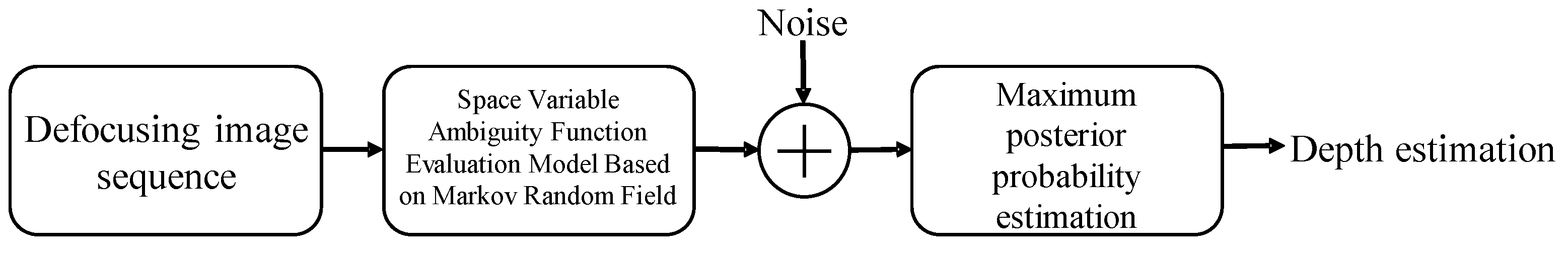
2.1. Depth Estimation Method Based on Markov Random Field

2.1.1. Markov Random Field Theory

In most image processing problems, the value of the desired pixel usually does not depend on pixels outside its immediate neighborhood, so the image signal can be regarded as a Markov random field [31,32].

Specifically, for the image $X$ we collected, the pixel point is set as $s$. The random variable $x_s$ is the implementation of $X_s$, $N_s$ is the neighborhood of $s$, and the pixel point is set as $S=\left\{s=\left(i,j\right):1\le i\le Q_1,1\le j\le Q_2\right\}$. If image $X$ satisfies:

$$P\left(X_s=x_s\right)>0$$

$$P(X_s=x_s|X_r=x_r,r\in S,r\ne s)=P(X_s=x_s|X_r=x_r,r\in N_S)$$

(1)

In this case, $x$ is the Markov random field of $N_s$.

2.1.2. Markov Random Field Defocusing Feature Model

We established the maximum posterior probability depth estimation model of a Markov random field (MRF) [33]. As shown in Figure 1, it is assumed that the MRF can express the defocused image and its blur parameters. Then, the blur parameters and the focused image are smoothed to improve the depth estimation quality. Thus, given two defocused images, the depth estimation and focus image restoration constitute the maximum a posteriori probability estimation problem.

$$g_k\left(i,j\right)={{\displaystyle \sum }}_m{{\displaystyle \sum }}_{n}f\left(m,n\right)h_k\left(i,j;m,n\right)+w_k\left(i,j\right),k=1,2$$

(2)

$g_1(\cdot )$ and $g_2(\cdot )$ represents two defocused images, the original focus image $f(\cdot )$ is unknown, and the ambiguity functions $h_1(\cdot )$ and $h_2(\cdot )$ are gaussian model ambiguity functions composed of blur parameters [34].

$k=1, 2$, ${\sigma }_{m,n_2}=\alpha {\sigma }_{m,n_1}+\beta$ and $\alpha , \beta$ are given parameters.

The parameter $S$ is regarded as the random field of blur parameter ${\sigma }_{m,n_1}$, while $F$ represents sliding windows (number: L) of a random field, corresponding to $N\times N$ focused image. Suppose $S$ could have $P$ possible levels and $F$ could have $M$ possible levels. $S$ and $F$ are continuous in the image scene, and their intensity can usually be quantified to 256 gray levels.

Quantization of blur parameters is necessary to reduce the configuration of the minimal posterior probability model. The mean and variance ${\sigma }_w^2$ of Gaussian white noise field $W1$ and $W2$ are set as zero. Similarly, assume that $S$ and $F$ are statistically independent of each other and are independent of $W1$ and $W2$. Let $G1$ and $G2$ represent the random field of the observed image.

Then, in Equation (2), $g_k$ can be expressed as in Equation (3):

$$g_k=H_{k}f+w_k,k=1,2$$

(3)

where the vectors $g_k$, $f$, and $w_k$ represent the matrices of $g_k\left(i,j\right)$, $f\left(i,j\right),$ and $w_k\left(i,j\right)$, respectively. The blur parameter matrix $H_k$ is composed of linear variable ambiguity functions $h_k\left(i,j;m,n\right)$. In Formula (3), the Gaussian blur window is set to have a limited space range ($\pm 3\sigma$ pixels).

The model also includes a linear field to maintain discontinuity in the blurring process and the image focus of the scene. The horizontal and vertical fields corresponding to the fuzzy process are respectively denoted by ${l^{\prime }}_{i,j}^s$ and ${v^{\prime }}_{i,j}^s$, while the linear fields corresponding to the intensity process are denoted by ${l^{\prime }}_{i,j}^f$, ${v^{\prime }}_{i,j}^f.$ Since both $S$ and $F$ are Markov random fields, that is MRF [33], there are Equations (4) and (5):

$$P[S=s,{L^{\prime }}^s={l^{\prime }}^s,{V^{\prime }}^s={v^{\prime }}^s]=\frac{1}{Z^s}{e}^{-U^s(s,{l^{\prime }}^s,{v^{\prime }}^s)}$$

(4)

$$P[F=f,{L^{\prime }}^f={l^{\prime }}^f,{V^{\prime }}^f={v^{\prime }}^f]=\frac{1}{Z^f}{e}^{-U^f(f,{l^{\prime }}^f,{v^{\prime }}^f)}$$

(5)

where $Z^s$,$Z^f$,$U^s(s,{l^{\prime }}^s,{v^{\prime }}^s)$, and $U^f(f,{l^{\prime }}^f,{v^{\prime }}^f)$ are:

$$Z^s={\displaystyle \sum }_{all(s,{l^{\prime }}^s,{v^{\prime }}^s)}{e}^{-U^s(s,{l^{\prime }}^s,{v^{\prime }}^s)}$$

$$Z^f={\displaystyle \sum }_{all(f,{l^{\prime }}^f,{v^{\prime }}^f)}{e}^{-U^f(f,{l^{\prime }}^f,{v^{\prime }}^f)}$$

$$U^s(s,{l^{\prime }}^s,{v^{\prime }}^s)={\displaystyle \sum }_{c\in C_s}{V}_c^s(s,{l^{\prime }}^s,{v^{\prime }}^s)$$

$$U^f(f,{l^{\prime }}^f,{v^{\prime }}^f)={\displaystyle \sum }_{c\in C_f}{V}_c^f(f,{l^{\prime }}^f,{v^{\prime }}^f)$$

$V_c^s(s,{l^{\prime }}^s,{v^{\prime }}^s)$ and $V_c^f(f,{l^{\prime }}^f,{v^{\prime }}^f)$ are the possible set functions related to $S$ and $F$, while $C_s$ and $C_f$ respectively represent the sequence set corresponding to $S$ and $F$.

2.1.3. Algorithm Implementation

To simplify the model representation method in the previous section, the blur parameter $\delta$ of the observed defocused image is regarded as a Markov random field, which is recorded as h. The probability $P\left(X\right)$ is shown in Equation (6):

$$P\left(X\right)=\frac{1}{z}{e}^{-{{\displaystyle \sum }}_{c\in C}{V}_c\left(x\right)}$$

(6)

where the Gibbs distribution is used to describe $P\left(X\right)$, and $y_1$, $y_2$, $P\left(Y_1=y_1,Y_2=y_2\right)$ is a constant.

The blur image $y$ is regarded as the convolution of the clear image $f$ and the point spread function $h$, as in Equation (7):

$$y_k\left(i,j\right)=h_k\left(i,j\right)\ast f\left(i,j\right) k=1,2$$

(7)

The point diffusion function $h_k\left(i,j\right)$ is a Gaussian function with blur parameters $\delta$, which reflects the radius of the dispersion circle.

Assume the MRF of the image of $y_i$ follows Equation (8):

$$y_i=f\left(x_i\right)+w_i$$

(8)

Here, $f\left(x_i\right)$ can be expressed as ${\mu }_x$, obtaining Equation (9):

$$P\left(Y_1=y_1,Y_2=y_2|X\right)=e^{-{{\displaystyle \sum }}_s\frac{1}{2{\delta }^2}{\left(y_1-{\mu }_1\right)}^2-{{\displaystyle \sum }}_s\frac{1}{2{\delta }^2}{\left(y_1-{\mu }_1\right)}^2}$$

(9)

Then, we can convert Equation (9) into (10):

$$P\left(X|Y_1=y_1,Y_2=y_2\right)=\frac{1}{z}{e}^{\left[{{\displaystyle \sum }}_{c\in C}{V}_c\left(x\right)-{{\displaystyle \sum }}_s\frac{1}{2{\delta }^2}{\left(y_1-{\mu }_1\right)}^2-{{\displaystyle \sum }}_s\frac{1}{2{\delta }^2}{\left(y_1-{\mu }_1\right)}^2\right]}$$

(10)

The posterior probability $P\left(X|Y_1,Y_2\right)$ of the original image will be transformed into the following optimization problem, as in Equation (11):

$$\mathit{min}\left[{\displaystyle \sum }_{c\in C}{V}_c\left(x\right)-{\displaystyle \sum }_s\frac{1}{2{\delta }^2}{\left(y_1-{\mu }_1\right)}^2-{\displaystyle \sum }_s\frac{1}{2{\delta }^2}{\left(y_2-{\mu }_2\right)}^2\right]$$

(11)

2.2. Modeling Depth Estimation Method Based on Geometric Constraints

According to the analysis in the previous section, we classified the problem as a DFD problem. The blur parameter difference model and its spatial constraint are deduced according to the difference between the focus plane and imaging position. This model can establish the relationship between depth information and blur information, and iteratively estimate the complete spatial information of the target object [35].

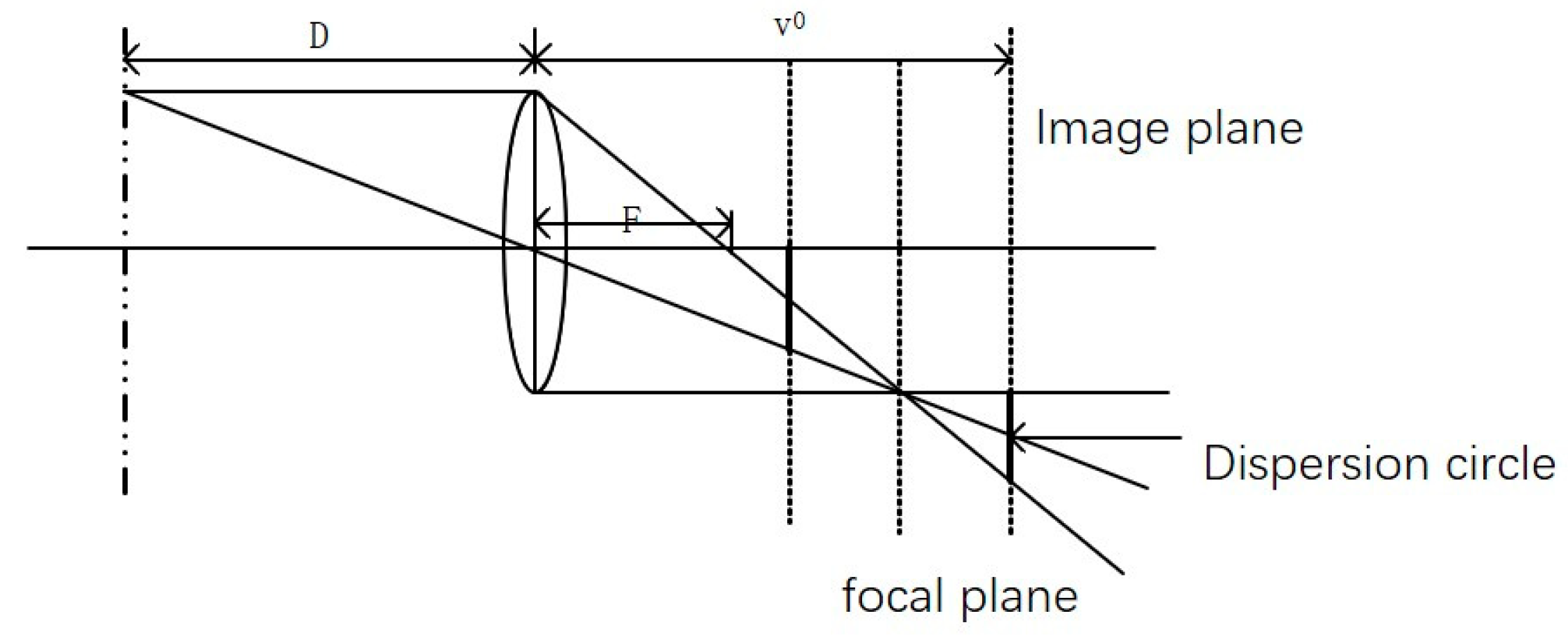
2.2.1. Geometric Derivation of the Depth Estimation Model

The geometric principle of real aperture imaging is shown in Figure 2. There are three position relations between the focal plane and the imaging plane: the image is on the focal plane ${\mathrm{v}}_0=\mathrm{v}$; the image is in front of the focal plane ${\mathrm{v}}^0<\mathrm{v}$; and the image is behind the focal plane ${\mathrm{v}}^0>\mathrm{v}$ [30].

The parameter $F$ stands for focal length, $D$ stands for object distance, and ${\mathrm{v}}^0$ stands for image distance when ${\mathrm{v}}^0=\mathrm{v}$, $\frac{1}{D}+\frac{1}{\mathrm{v}}=\frac{1}{F}.$

When ${\mathrm{v}}^0<\mathrm{v}$, $\frac{1}{F}<\frac{1}{D}+\frac{1}{{\mathrm{v}}^0}$, set $r_0$ as the radius of the lens; the radius of the dispersion circle is shown in Equation (12):

$$r=r_0 {\mathrm{v}}^0\left(\frac{1}{{\mathrm{v}}^0}+\frac{1}{D}-\frac{1}{F}\right)$$

(12)

when ${\mathrm{v}}^0<\mathrm{v},\frac{1}{F}>\frac{1}{D}+\frac{1}{{\mathrm{v}}^0}$. The radius of the dispersion circle is shown in Equation (13):

$$r=r_0 {\mathrm{v}}^0\left(\frac{1}{F}-\frac{1}{{\mathrm{v}}^0}-\frac{1}{D}\right)$$

(13)

From Equations (12) and (13), the radius of the dispersion circle, namely the blur degree evaluation parameter, can be expressed as in Equation (14):

$$r=r_0 {\mathrm{v}}^0\left|\frac{1}{F}-\frac{1}{{\mathrm{v}}^0}-\frac{1}{D}\right|$$

(14)

Since the radius of the dispersion circle has a certain relationship with the camera, in consideration of this point, let $r\rho =\sigma$. The blur parameter $\sigma$ is as in Equation (15):

$$\sigma =\rho r_0 {\mathrm{v}}^0\left|\frac{1}{F}-\frac{1}{{\mathrm{v}}^0}-\frac{1}{D}\right|$$

(15)

The parameter $\sigma$ is also a diffusion parameter that measures the point spread function (PSF) of the dispersion circle. Take the Gaussian diffusion function as an example. It can be expressed as in Equation (16):

$$h_{\sigma }{}^u\left(y,x\right)=\frac{1}{2\pi {\sigma }^2}{e}^{-\frac{\Vert y-x{\Vert }^2}{2{\sigma }^2}}$$

(16)

where the relevant parameters of the camera are set as $u$ and the function is denoted by $h_{\sigma }^u\left(y,x\right)$.

Firstly, the two defocused images were studied and the generated defocused images ${\tilde{I}}_1$ and ${\tilde{I}}_2;$ their expressions were as follows:

Here, we study the situation of two defocused images. Images $I_1$ and $I_2$ are collected and the generated defocused images ${\tilde{I}}_1$ and ${\tilde{I}}_2$ are expressed as in Equations (17) and (18):

$${\tilde{I}}_1\left(y\right)={{\displaystyle \int }}_{\Omega }{h}_{{\sigma }_1}^{u_1}\left(y,x\right)f\left(x\right)dx$$

(17)

$${\tilde{I}}_2\left(y\right)={{\displaystyle \int }}_{\Omega }{h}_{{\sigma }_2}^{u_2}\left(y,x\right)f\left(x\right)dx$$

(18)

where $u_1$ and $u_2$ represent the parameters of the camera while shooting the image $I_1$ and $I_2$; ${\sigma }_1$ and ${\sigma }_2$ represent the diffusion parameters of the ambiguity function.

Use the difference function to simulate the difference in the degree of blur of the two images at different positions, as shown in Equation (19):

$$\tilde{f},\tilde{\sigma }=argmin \Phi \left(f,\sigma \right)$$

(19)

The approximation method adopts the least square method, as shown in Equation (20):

$$\Phi \left(f,\sigma \right)={{\displaystyle \int }}_{\Omega }\Vert I\left(y\right){\tilde{I}}_{\sigma }^u\left(y\right)\Vert dy={{\displaystyle \int }}_{\Omega }\Vert I\left(y\right)-{{\displaystyle \int }}_{\Omega }{h}_{{\sigma }_2}^{u_2}\left(y,x\right)f\left(x\right)dx{\Vert }_2^{2}dy$$

(20)

Least squares filtering requires the variance and mean of noise, and these parameters can be calculated from a given degraded image, which is an important advantage of constrained least squares filtering.

Set two $PSF$ functions as $h_{{\sigma }_1}\left(x,y\right)=\frac{1}{2\pi {\sigma }_1^2}{e}^{-\frac{x^2+y^2}{2{\delta }_1^2}} \mathrm{and} h_{{\sigma }_2}\left(x,y\right)=\frac{1}{2\pi {\sigma }_2^2}{e}^{-\frac{x^2+y^2}{2{\delta }_2^2}}$; then, we obtain Equation (21):

$$h_{{\sigma }_3}\left(x,y\right)=h_{{\sigma }_1}\left(x,y\right)\times h_{{\sigma }_2}\left(x,y\right)=\frac{1}{2\pi \left({\sigma }_1^2+{\sigma }_2^2\right)}{e}^{-\frac{x^2+y^2}{2\left({\delta }_1^2+{\delta }_2^2\right)}}$$

(21)

The parameters ${\sigma }_1$, ${\sigma }_2$, and ${\sigma }_3$ of the PSF functions $h_{{\sigma }_1}\left(x,y\right)$, $h_{{\sigma }_2}\left(x,y\right)$, $h_{{\sigma }_3}\left(x,y\right)$ satisfy ${\sigma }_1^2<{\sigma }_3^2$. Among them, $h_{{\sigma }_1}\left(x,y\right)$ and $h_{{\sigma }_2}\left(x,y\right)$ are convolved to obtain $h_{{\sigma }_3}\left(x,y\right)$, and ${\sigma }_2=\sqrt{{\sigma }_3^2-{\sigma }_1^2}$ is the parameter of $h_{{\sigma }_2}\left(x,y\right)$.

According to the different heights of the object being observed, the blur degree of each area of the two images can be expressed as $\Sigma =\left\{y:{\sigma }_1^2>{\sigma }_2^2\right\}$ and ${\Sigma }^c=\left\{y:{\sigma }_1^2<{\sigma }_2^2\right\}$.

In $y\in \Sigma =\left\{y:{\sigma }_1^2>{\sigma }_2^2\right\}$, the collected scatter image $I_1$’s blur process can be simulated as in Equation (22):

$${\stackrel{◠}{I}}_1\left(y\right)={\displaystyle \int } h_{{\sigma }_1}\left(y,x\right)f\left(x\right)dx\cong {\displaystyle \int } h_{\Delta \sigma }\left(y,\overline{y}\right)I_2\left(y\right)dy$$

(22)

where $\Delta \sigma =\sqrt{{\sigma }_1^2-{\sigma }_2^2}$.

In $y\in \Sigma =\left\{y:{\sigma }_1^2<{\sigma }_2^2\right\}$, the collected scatter image $I_2$’s blur process can be simulated as in Equation (23):

$${\stackrel{◠}{I}}_2\left(y\right)={\displaystyle \int } h_{{\sigma }_2}\left(y,x\right)f\left(x\right)dx\cong {\displaystyle \int } h_{\Delta \sigma }\left(y,\overline{y}\right)I_1\left(y\right)dy$$

(23)

where $\Delta \sigma =-\sqrt{{\sigma }_2^2-{\sigma }_1^2}$.

Construct the functional extremum function as shown in Equation (24):

$$\Delta \stackrel{◠}{\sigma }=\underset{\Delta \sigma }{argmin}\Phi \left(\Delta \sigma \right)$$

(24)

Similarly, the least square method is also used to simulate, as shown in Equation (25):

$$\begin{array}{l}\Phi \left(\Delta \sigma \right)={{\displaystyle \int }}_{\Sigma }\Vert {\stackrel{◠}{I}}_1\left(y\right)-I_1\left(y\right){\Vert }_2^{2}dy+{{\displaystyle \int }}_{{\Sigma }^c}\Vert {\stackrel{◠}{I}}_2\left(y\right)+I_2\left(y\right){\Vert }_2^{2}dy\\ ={\displaystyle \int } H\left(\Delta \left(y\right)\right)\Vert {\stackrel{◠}{I}}_1\left(y\right)-I_1\left(y\right){\Vert }_2^{2}dy+{\displaystyle \int } \left(1-H\left(\Delta \left(y\right)\right)\right)\Vert {\stackrel{◠}{I}}_2\left(y\right)+I_2\left(y\right){\Vert }_2^{2}dy\end{array}$$

(25)

Establish the relationship between $\Delta \sigma$ and $D$:

$$\{\begin{array}{c}{\sigma }_1^2={\rho }^2{r}_0^0{v}_1^2{\left(\frac{1}{F}-\frac{1}{v_1}-\frac{1}{D}\right)}^2\\ {\sigma }_2^2={\rho }^2{r}_0^0{v}_2^2{\left(\frac{1}{F}-\frac{1}{v_2}-\frac{1}{D}\right)}^2\end{array}$$

(26)

After the operation, we can obtain Equation (27):

$$\frac{1}{\left(v_1-v_2\right)\left(v_1+v_2\right)}\frac{\Delta \sigma \left|\Delta \sigma \right|}{{\rho }^2{r}_0^2}={\left(\frac{1}{F}-\frac{1}{D}\right)}^2-\frac{2}{v_1+v_2}\left(\frac{1}{F}-\frac{1}{D}\right)$$

(27)

By solving Equation (27), we obtain Equation (28):

$$\frac{1}{F}-\frac{1}{D}=\frac{1}{v_1+v_2}\pm \frac{1}{v_1+v_2}\sqrt{1+\frac{\Delta \sigma \left|\Delta \sigma \right|}{{\rho }^2{r}_0^2}\cdot \frac{v_1+v_2}{v_1-v_2}}$$

(28)

Finally, the mapping between $\Delta \sigma$ and $D$ is established, as shown in Equation (29):

$$D\left(y\right)={\left(\frac{1}{F}-\frac{1}{v_1+v_2}-\frac{1}{v_1+v_2}\sqrt{1+\frac{\Delta \sigma \left(y\right)\left|\Delta \sigma \left(y\right)\right|}{{\rho }^2{r}_0^2}\cdot \frac{v_1-v_2}{v_1-v_2}}\right)}^{-1}$$

(29)

According to the positional relationship between the focal plane and the imaging plane of the image taken by the camera, four position situations can be obtained:

(1)

When $F<v<v_1$, we can obtain Equations (30) and (31):

$$F<\frac{1}{F}-\frac{1}{D}<v_1$$

(30)

$$F<\frac{1}{v_1+v_2}+\frac{1}{v_1+v_2}\sqrt{1+\frac{\Delta \sigma \left|\Delta \sigma \right|}{{\rho }^2{r}_0^2}\cdot \frac{v_1+v_2}{v_1-v_2}}<v_1$$

(31)

The inequality relationship of $\Delta \sigma \left|\Delta \sigma \right|$ is shown in Equation (32):

$${\rho }^2{r}_0^2\frac{v_1-v_2}{v_1+v_2}\left[{\left(\frac{v_1+v_2}{F}\right)}^2-\frac{2\left(v_1-v_2\right)}{F}\right]<\Delta \sigma \left|\Delta \sigma \right|<{\rho }^2{r}_0^2\frac{v_1-v_2}{v_1+v_2}\left(\frac{v_2^2}{v_1^2}-1\right)$$

(32)

(2)

When $v_2<v<2F$. The inequality relationship of $\Delta \sigma \left|\Delta \sigma \right|$ is shown in Equation (33):

$${\rho }^2{r}_0^2\frac{v_1-v_2}{v_1+v_2}\left(\frac{v_2^2}{v_1^2}-1\right)<\Delta \sigma \left|\Delta \sigma \right|<{\rho }^2{r}_0^2\frac{v_1-v_2}{v_1+v_2}\left[{\left(\frac{v_1+v_2}{2F}\right)}^2-\frac{\left(v_1+v_2\right)}{F}\right]$$

(33)

(3)

When $v_1<v<\frac{v_1+v_2}{2}$. The inequality relationship of $\Delta \sigma \left|\Delta \sigma \right|$ is shown in Equation (34):

$${\rho }^2{r}_0^2\frac{v_1-v_2}{v_1+v_2}\left(\frac{v_2^2}{v_1^2}-1\right)<\Delta \sigma \left|\Delta \sigma \right|<0$$

(34)

(4)

When $\frac{v_1+v_2}{2}<v<v_2$. The inequality relationship of $\Delta \sigma \left|\Delta \sigma \right|$ is shown in Equation (35):

$$0<\Delta \sigma \left|\Delta \sigma \right|<{\rho }^2{r}_0^2\frac{v_1-v_2}{v_1+v_2}\left(\frac{v_2^2}{v_1^2}-1\right)$$

(35)

As can be seen from the above, $\Delta \sigma$ is taken negatively in (1) and (3); $y\in {\Sigma }^c=\left\{y:{\sigma }_1^2<{\sigma }_2^2\right\}$ and then execute $y\in \Sigma =\left\{y:{\sigma }_1^2>{\sigma }_2^2\right\}$.

As can be seen from Figure 2, all observed defocused images satisfy $F<v<2F$. Then, the inequality relationship of $\Delta \sigma \left|\Delta \sigma \right|$ is shown in Equation (36):

$$\begin{gathered} {\rho }^2{r}_0^2\frac{v_1-v_2}{v_1+v_2}\left[\left(\frac{v_1+v_2}{F}\right)-\frac{2\left(v_1+v_2\right)}{F}\right]<\Delta \sigma \left|\Delta \sigma \right| \\ \hspace{1em}\hspace{1em}\hspace{1em}\hspace{1em}\hspace{1em}\hspace{1em}\hspace{1em}\hspace{1em}<{\rho }^2{r}_0^2\frac{v_1-v_2}{v_1+v_2}\left[{\left(\frac{v_1+v_2}{2F}\right)}^2-\frac{\left(v_1+v_2\right)}{F}\right] \end{gathered}$$

(36)

From Equations (12) and (28), we obtain the objective function and the constraints of the optimization problem, respectively.

The depth estimation model is as in Equation (37):

$$\begin{array}{l}\underset{\Delta \sigma }{min}{\displaystyle \int } H\left(\Delta \sigma \left(y\right)\right)\Vert {\stackrel{◠}{I}}_1\left(y\right)-I_1\left(y\right){\Vert }_2^{2}dy+{\displaystyle \int } \left(1-H\left(\Delta \sigma \left(y\right)\right)\right)\Vert {\stackrel{◠}{I}}_2\left(y\right)-I_2\left(y\right){\Vert }_2^{2}dy\\ s.t. {\rho }^2{r}_0^2\frac{v_1-v_2}{v_1+v_2}\left[\left(\frac{v_1+v_2}{F}\right)-\frac{2\left(v_1+v_2\right)}{F}\right]<\Delta \sigma \left|\Delta \sigma \right|\\ \hspace{1em}\hspace{1em}\hspace{1em}\hspace{1em}\hspace{1em}\hspace{0.17em}<{\rho }^2{r}_0^2\frac{v_1-v_2}{v_1+v_2}\left[{\left(\frac{v_1+v_2}{2F}\right)}^2-\frac{\left(v_1+v_2\right)}{F}\right]\end{array}$$

(37)

2.2.2. An Improved Depth Estimation Algorithm for Defocused Images

Since the objective function of Equation (36) is monotonic, the exhaustive method is used to check the minimum value in the process of depth estimation. The basic steps of the multi-scale minimum exhaustion method are as follows:

(1)

According to the four types of imaging geometric relationships described in the previous section (Equations (30)–(35)), for the two acquired defocused images that determine the camera parameters, determine the $\Delta \sigma$ preliminary interval $\left[\alpha ,\beta \right]$;

(2)

The interval $\left[\alpha ,\beta \right]$ for determining camera parameters is discretized according to $N$ points, as shown in Equation (38):

$$\alpha =\Delta {\sigma }_0<\Delta {\sigma }_1<\dots <\Delta {\sigma }_n=\beta$$

(38)

(3)

For the $\underset{k\in \left\{0,1,\dots ,n\right\}}{\Delta {\sigma }_{\ast }=argmin\left(\Phi \left(\Delta {\sigma }_k\right)\right)}$ in Equation (25), obtain the $\Delta {\sigma }_{*}$ make $\Phi \left(\Delta {\sigma }_k\right), \mathrm{and}$ obtain the smallest value;

(4)

For the two points on the left and right of $\Delta {\sigma }_{*}$, let $\alpha =\Delta {\sigma }_{*-1}$ and $\beta =\Delta {\sigma }_{*+1},$ respectively; according to the set threshold $\epsilon$, judge $\left|\alpha -\beta \right|\ge \epsilon$. If its value is true, then cycle (2)–(4) steps; if it is false, take it as the minimum value of Equation (25).

(5)

The depth information is estimated according to Equation (37).

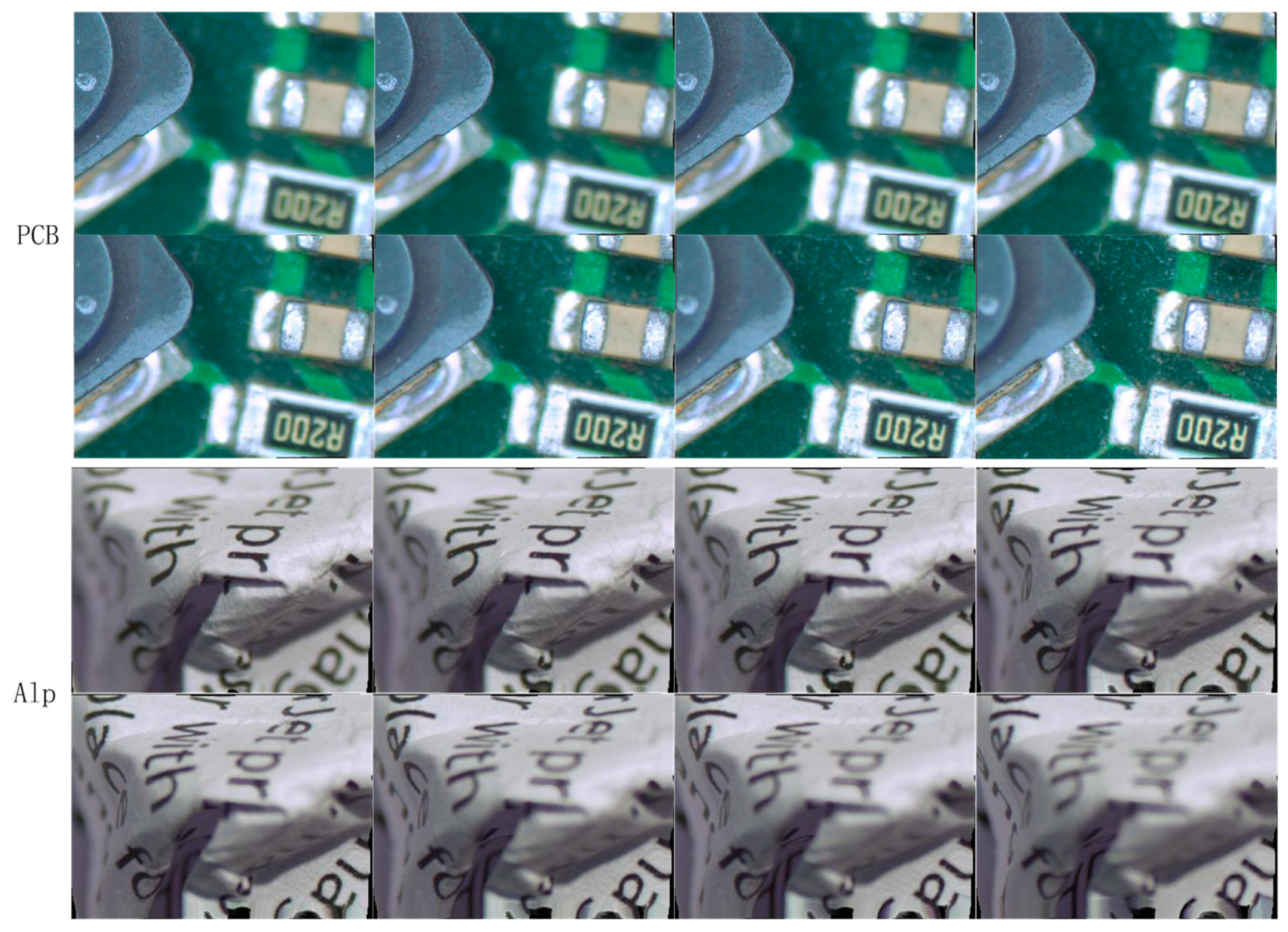
3. Results

The experimental environment of this research is introduced as follows:

• One PC with: CPU: i7-9700K, GPU: RTX2060S, RAM: 16G, ROM: 516GSSD;
• One ByslorPylon industrial camera, model: acA640-120 uc;
• A monocular microscope with a magnification of 0.5 × (0.7~4.5), a lens radius of 35 mm, and an F number of 4.

All experiments in this article were completed under the Windows 10 operating system, using Bysler’s PylonViewer to collect images under the microscope, and to simulate through Matlab2016a. A small part of the preprocessing steps used Microsoft Visual Studio 2013 and OpenCV.

The purpose of this study is to determine a relatively accurate 3D model of the target object by using depth estimation of multiple defocused images shot by an electronic video microscope [36]. Therefore, an estimation model is designed to estimate depth information using the multi-frame defocus image model in this experiment. The steps are as follows:

(1)

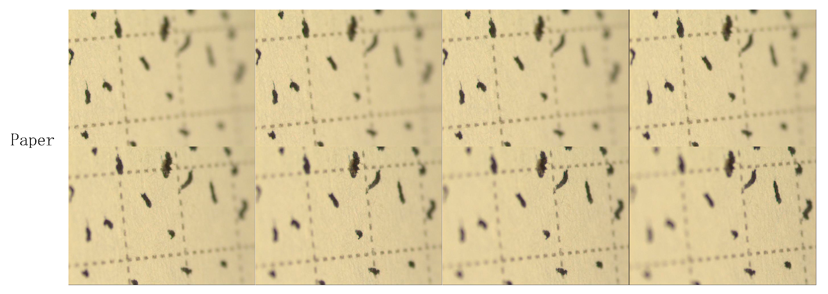
The sequence of collected images are numbered as $I_1$, $I_2$, $I_3$, …, $I_N.$ Set a value K so that the collected image sequence, according to $\left(I_1,I_K\right)$, $\left(I_2,I_{K+1}\right)$, ……, $\left(I_K,I_{N-K}\right),$ respectively. Estimate depth information according to the algorithm in the previous section;

(2)

For the estimated results $D_1$, $D_2$, ……, $D_{N-K}$, the depth value of each pixel in n-k matrices is used as the histogram. Then, the greatest depth value (or the most concentrated value) is selected as the point’s depth. Thus, the new fusion depth information is finally obtained.

We first use a microscope and a Basler industrial camera acA640 to take two sets of defocused images, PCB and Alp, as shown in Figure 3.

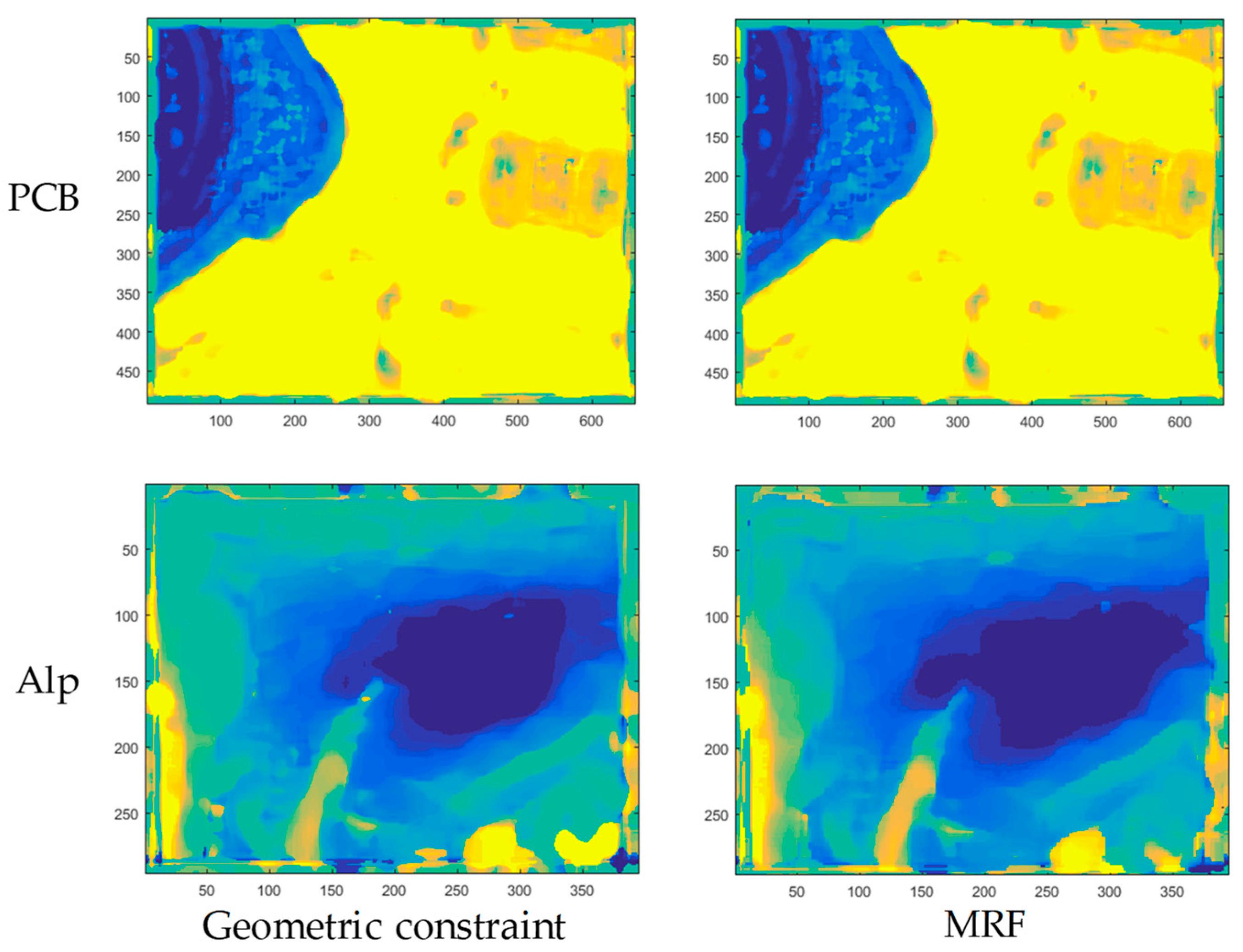
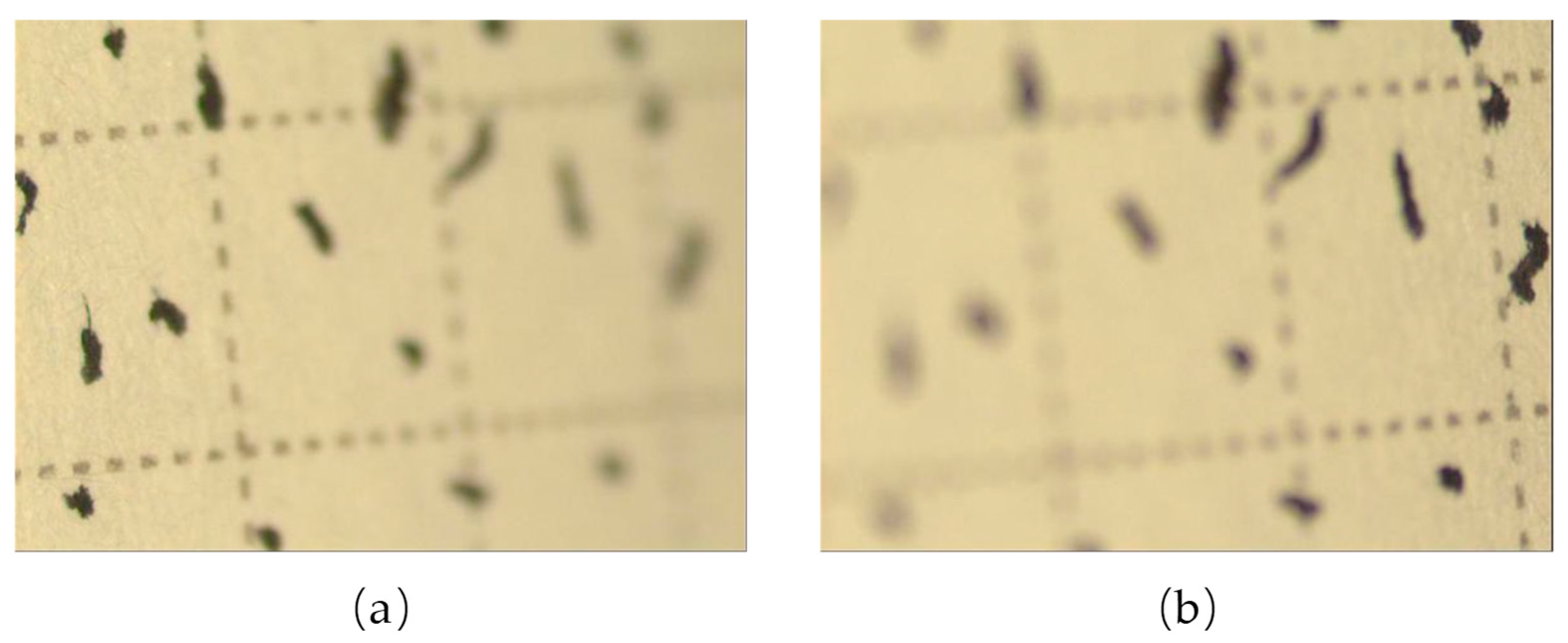
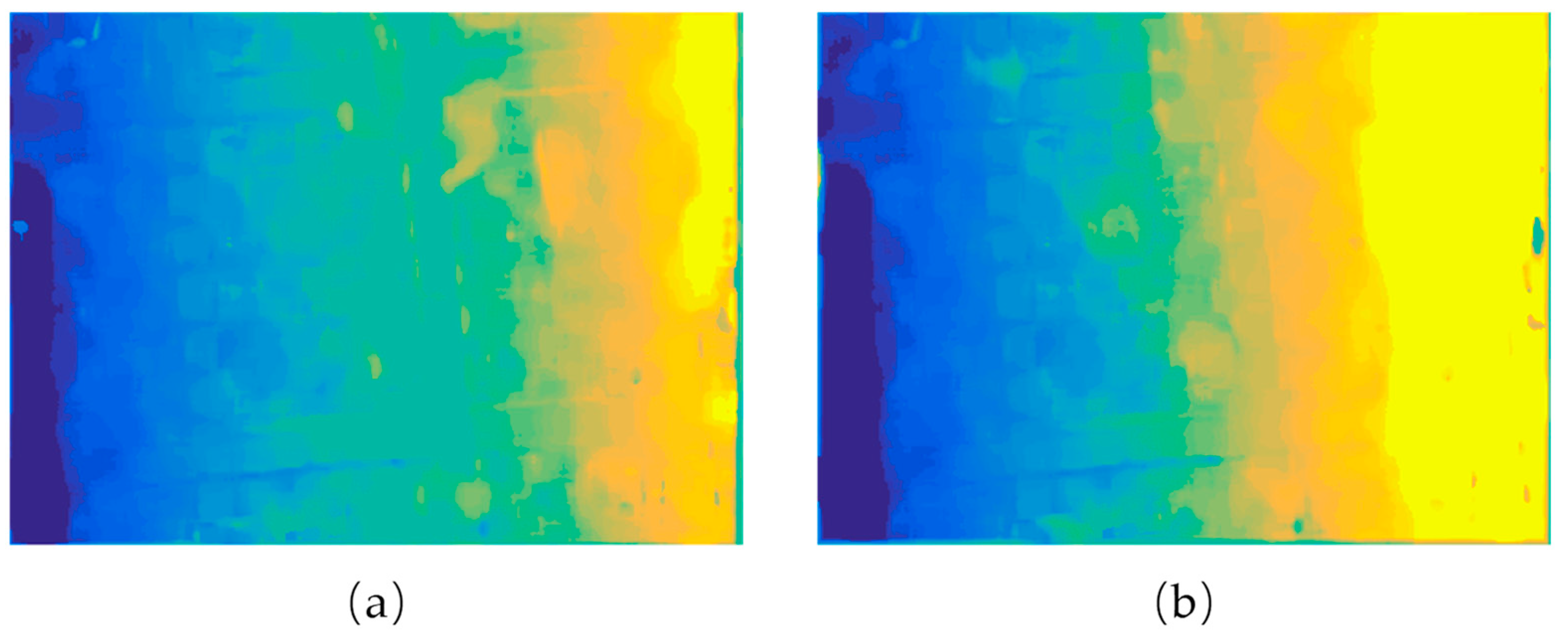
3.1. The Effects of Geometric Constraint-Based Method and MRF Method

We calculated the depth maps of PCB and Alp defocused images using the geometric constraint-based algorithm and MRF depth estimation algorithm, respectively. The results are shown in Figure 4.

In the two sets of depth maps, you can see that the effect of the geometric constraint method is similar to the result of the MRF method. However, its running time is quite different. This because the algorithm based on geometric constraints has a lower algorithm complexity. Therefore, its running time is much shorter than that of the MRF algorithm.

3.2. Gradient Characteristics Simulation

We photographed the paper data group with gradient characteristics, as shown in Figure 5. The height of both pictures decreases from left to right. Because of the different focal lengths, the clear areas of the two images are different. Figure 5a is near focal length and Figure 5b is far focal length.

Using geometric constraints and MRF methods to estimate the gradient scene, the results are shown in Figure 6.

We made a quantitative comparison of the results, divided the gradient image into 22 columns, and obtained each column’s average true depth and estimated depth, as shown in Figure 7a,b.

3.3. Accuracy and Efficiency Analysis

It can be seen from the figure that the geometric constraint method has more significant advantages than the MRF method in terms of smoothness and accuracy.

In order to analyze the accuracy and efficiency of the two methods synthetically with quantitative indexes, the square root of mean square error, the root mean square (RMS), is used to quantify the accuracy, as in Equation (39):

$$\mathrm{RMS}=\sqrt{\frac{1}{N\left(\Omega \right)}{\displaystyle \sum }_{\left(i,j\right)\in \Omega }[\stackrel{◠}{d}\left(i,j\right)-d\left(i,j\right)]}$$

(39)

Table 1. The running times and the square roots of the mean square error of the two methods were compared and analyzed at the paper data source.

Geometric Constraints		MRF
RMS	Running Time	RMS	Running Time
3.3318	53.93	5.0129	197.4923

shows the running time (s) and RMS of the two methods with the paper data.

Experiments proved that the accuracy of the depth estimation method based on geometric constraints is slightly higher than the MRF method. Furthermore, its running time is significantly better than that of the MRF method.

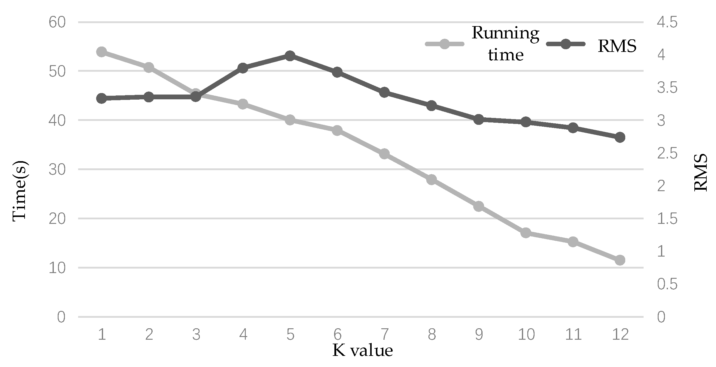
3.4. Selection of K Value in the Geometrically Constrained Improved Depth Estimation Algorithm

For depth estimation methods based on geometric constraints, experiments are supplemented to illustrate the comparison of the depth estimation effects of the algorithms when K is a different value. The registered paper data group is used, as shown in Figure 8.

The experimental results are shown in

Table 2. Comparative analysis of depth estimation based on geometric constraints.

Value of K	1	2	3	4	5	6
RMS	3.3318	3.3533	3.3597	3.7966	3.9827	3.7321
Running time	53.93	50.77	45.39	43.29	40.08	37.92
Value of K	7	8	9	10	11	12
RMS	3.4251	3.2219	3.0121	2.9739	2.8847	2.7396
Running time	33.19	27.91	22.49	17.11	15.29	11.53

and Figure 9.

Because the larger the K value, the smaller the number of experimental groups, the K value does not have much effect on the overall running time. The difference in this value is mainly due to the number of experimental groups with increasingly smaller K values. As far as the estimated effect is concerned, when K takes small and large values, the RMS value is not high. However, when K = 5, the RMS index is the highest, the difference of the acquired depth information is the most obvious, and the utilization of the blur information in the defocused image sequence is better. Therefore, experiments show that depth estimation works best when this value is taken.

4. Discussion

This study fits the operating efficiency and effect of the geometric constraint method with simulation data to obtain more reliable data. It is verified that the geometric constraint method has higher runtime efficiency.

During the experiment, it was found that the depth estimation of the PCB image sequence has a significant error, and the depth of the reflective metal surface and the surrounding area does not match the actual depth. This is because the reflection creates errors in the detection of the feature points. Therefore, the conclusion is drawn that this type of DFD method has certain requirements for the object’s surface characteristics and lighting conditions to obtain depth information.

In the two sets of depth maps, the effect of the geometric constraint method is similar to that of the MRF method. However, the running time of algorithms based on geometric constraints is quite different. Due to the algorithm’s low complexity, the running time of the algorithm based on geometric constraints is much shorter than that of the MRF algorithm. The experimental results show that the geometric constraint method has greater advantages in smoothness and accuracy than the MRF method. The specific reason may be that in millimeter-scale scenes, there are fewer picture features. Using Markov random fields to describe the relationship between the depth of a pixel or region and the depth of its neighboring pixels or regions does not work well, resulting in reduced accuracy and smoothness.

For the selection of the K value, according to the experimental results, the larger the K value, the smaller the experimental group and the shorter the running time. This is a simple linear relationship. For example, when the K value is 3, there are only nine sets of depth information, and when the K value is 12, there is only one set.

Therefore, our choice of K value depends to a large extent on the accuracy requirements. When K is small, such as K = 1, the ambiguity difference of the radius of the estimated dispersion circle is too small, and accuracy cannot be guaranteed. The larger the K, the greater the accuracy. The K value is the middle number between the first 30% to 40% of the number of out-of-focus image sequences, and the effect is better.

There are various methods to improve the computational efficiency and depth estimation effect. However, the operation time is still far from real-time operation speed at the ms level. One may try to use CUDA programming to speed up the operation. Through the optimization of the underlying operation method and the hardware GPUization of the operation, the algorithm can be further optimized, leading to corresponding improvements to its real-time performance. In the follow-up research, the main goal will be to improve computing efficiency and reduce the response time.

5. Conclusions

This article involves two methods to solve the problem of depth estimation of defocused images in microscopic scenes. Among them, the method based on geometric constraints uses the principle of real aperture imaging to derive the optimization model of the point spread function. Then, the constraint conditions are deduced through the inequality of the blur parameters under the different relationships between the imaging plane and the focus plane, and the final geometry-based constrained optimization model.

Secondly, for this type of defocused image depth estimation method, a relative disparity estimation of two images is used to improve a relatively accurate depth information estimation suitable for multiple images. Finally, the value of the improved parameter and its evaluation index was obtained through experimental analysis.

In this study, a depth estimation method using defocused images based on Markov random field was studied and simulated. Through the comparison between the Markov method and the geometric constraint method, it was found that the geometric constraint method has obvious advantages in operation efficiency. The method used in the article has a significant improvement in smoothness and accuracy compared to the Markov method; the RMS is reduced from 5.01 to 3.33 and the running time is also reduced to about a quarter of the Markov method’s running time.

References

1. Roberts, L.G. Machine Perception of Three-Dimensional Solids; Massachusetts Institute of Technology: Cambridge, MA, USA, 1963. [Google Scholar]
2. Ni, X.; Yin, L.; Chen, X.; Liu, S.; Yang, B.; Zheng, W. Semantic representation for visual reasoning. MATEC Web Conf. EDP Sci. 2019, 277, 02006. [Google Scholar] [CrossRef]
3. Huang, W.; Zheng, W.; Mo, L. Distributed robust H∞ composite-rotating consensus of second-order multi-agent systems. Int. J. Distrib. Sens. Netw. 2017, 13, 1550147717722513. [Google Scholar] [CrossRef]
4. Liu, S.; Wang, L.; Liu, H.; Su, H.; Li, X.; Zheng, W. Deriving bathymetry from optical images with a localized neural network algorithm. IEEE Trans. Geosci. Remote Sens. 2018, 56, 5334–5342. [Google Scholar] [CrossRef]
5. Esteban, C.H.; Schmitt, F. Silhouette and stereo fusion for 3D object modeling. Comput. Vis. Image Underst. 2004, 96, 367–392. [Google Scholar] [CrossRef] [Green Version]
6. Li, H.; Chai, Y.; Li, Z. Multi-focus image fusion based on nonsubsampled contourlet transform and focused regions detection. Optik 2013, 124, 40–51. [Google Scholar] [CrossRef]
7. Marr, D. Vision: A Computational Investigation into the Human Representation and Processing of Visual Information; MIT Press: Cambridge, MA, USA, 2010. [Google Scholar]
8. Ding, Y.; Tian, X.; Yin, L.; Chen, X.; Liu, S.; Yang, B.; Zheng, W. Multi-scale relation network for few-shot learning based on meta-learning. In Computer Vision Systems, Proceedings of the International Conference on Computer Vision Systems, Thessaloniki, Greece, 23–25 September 2019; Springer: Cham, Switzerland, 2019; pp. 343–352. [Google Scholar]
9. Li, S.; Kang, X.; Hu, J.; Yang, B. Image matting for fusion of multi-focus images in dynamic scenes. Inf. Fusion 2013, 14, 147–162. [Google Scholar] [CrossRef]
10. Tang, Y.; Liu, S.; Deng, Y.; Zhang, Y.; Yin, L.; Zheng, W. Construction of force haptic reappearance system based on Geomagic Touch haptic device. Comput. Methods Programs Biomed. 2020, 190, 105344. [Google Scholar] [CrossRef]
11. Subbarao, M.; Surya, G. Depth from defocus: A spatial domain approach. Int. J. Comput. Vis. 1994, 13, 271–294. [Google Scholar] [CrossRef]
12. Surya, G.; Subbarao, M. Depth from defocus by changing camera aperture: A spatial domain approach. In Proceedings of the IEEE Conference on Computer Vision and Pattern Recognition, IEEE, New York, NY, USA, 15–17 June 1993; pp. 61–67. [Google Scholar]
13. Subbarao, M.; Wei, T.-C. Depth from defocus and rapid autofocusing: A practical approach. In Proceedings of the 1992 IEEE Computer Society Conference on Computer Vision and Pattern Recognition, Champaign, IL, USA, 15–18 June 1992; pp. 773–776. [Google Scholar]
14. Zhou, C.; Lin, S.; Nayar, S.K. Coded aperture pairs for depth from defocus and defocus deblurring. Int. J. Comput. Vis. 2011, 93, 53–72. [Google Scholar] [CrossRef] [Green Version]
15. Costeira, J.; Kanade, T. A multi-body factorization method for motion analysis. In Proceedings of the IEEE International Conference on Computer Vision, Cambridge, MA, USA, 20–23 June 1995; pp. 1071–1076. [Google Scholar]
16. Irani, M. Multi-frame optical flow estimation using subspace constraints. In Proceedings of the Seventh IEEE International Conference on Computer Vision, Kerkyra, Greece, 20–27 September 1999; pp. 626–633. [Google Scholar]
17. Torresani, L.; Hertzmann, A.; Bregler, C. Nonrigid structure-from-motion: Estimating shape and motion with hierarchical priors. IEEE Trans. Pattern Anal. Mach. Intell. 2008, 30, 878–892. [Google Scholar] [CrossRef]
18. Brand, W. Morphable 3D models from video. In Proceedings of the 2001 IEEE Computer Society Conference on Computer Vision and Pattern Recognition, CVPR 2001, Kauai, HI, USA, 8–14 December 2001; p. II. [Google Scholar]
19. Li, Y.; Zheng, W.; Liu, X.; Mou, Y.; Yin, L.; Yang, B. Research and improvement of feature detection algorithm based on FAST. Rend. Lincei. Sci. Fis. E Nat. 2021, 32, 775–789. [Google Scholar] [CrossRef]
20. Newcombe, R.A.; Izadi, S.; Hilliges, O.; Molyneaux, D.; Kim, D.; Davison, A.J.; Kohi, P.; Shotton, J. Real-time dense surface mapping and tracking. In Proceedings of the 2011 10th IEEE International Symposium on Mixed and Augmented Reality, Washington, DC, USA, 26–29 October 2011; pp. 127–136. [Google Scholar]
21. Xu, C.; Yang, B.; Guo, F.; Zheng, W.; Poignet, P. Sparse-view CBCT reconstruction via weighted Schatten p-norm minimization. Opt. Express 2020, 28, 35469–35482. [Google Scholar] [CrossRef] [PubMed]
22. Marr, D.; Poggio, T. A computational theory of human stereo vision. Proc. R. Soc. London Ser. B Biol. Sci. 1979, 204, 301–328. [Google Scholar]
23. Huang, W.; Jing, Z. Evaluation of focus measures in multi-focus image fusion. Pattern Recognit. Lett. 2007, 28, 493–500. [Google Scholar] [CrossRef]
24. Huang, W.; Jing, Z. Multi-focus image fusion using pulse coupled neural network. Pattern Recognit. Lett. 2007, 28, 1123–1132. [Google Scholar] [CrossRef]
25. Tian, J.; Chen, L. Adaptive multi-focus image fusion using a wavelet-based statistical sharpness measure. Signal. Process. 2012, 92, 2137–2146. [Google Scholar] [CrossRef]
26. Wang, Z.; Ma, Y.; Gu, J. Multi-focus image fusion using PCNN. Pattern Recognit. 2010, 43, 2003–2016. [Google Scholar] [CrossRef]
27. Yang, B.; Liu, C.; Huang, K.; Zheng, W. A triangular radial cubic spline deformation model for efficient 3D beating heart tracking. Signal. Image Video Process. 2017, 11, 1329–1336. [Google Scholar] [CrossRef] [Green Version]
28. Yang, B.; Liu, C.; Zheng, W.; Liu, S. Motion prediction via online instantaneous frequency estimation for vision-based beating heart tracking. Inf. Fusion 2017, 35, 58–67. [Google Scholar] [CrossRef]
29. Zhou, Y.; Zheng, W.; Shen, Z. A New Algorithm for Distributed Control Problem with Shortest-Distance Constraints. Math. Probl. Eng. 2016, 2016, 1604824. [Google Scholar] [CrossRef]
30. Zheng, W.; Li, X.; Yin, L.; Wang, Y. The retrieved urban LST in Beijing based on TM, HJ-1B and MODIS. Arab. J. Sci. Eng. 2016, 41, 2325–2332. [Google Scholar] [CrossRef]
31. Chaudhuri, S.; Rajagopalan, A.N. Depth from Defocus: A Real Aperture Imaging Approach; Springer Science & Business Media: Berlin/Heidelberg, Germany, 2012. [Google Scholar]
32. Schechner, Y.Y.; Kiryati, N. Depth from defocus vs. stereo: How different really are they? Int. J. Comput. Vis. 2000, 39, 141–162. [Google Scholar] [CrossRef]
33. Ziou, D.; Deschenes, F. Depth from defocus estimation in spatial domain. Comput. Vis. Image Underst. 2001, 81, 143–165. [Google Scholar] [CrossRef]
34. Nourbakhsh, I.R.; Andre, D. Generating Categorical Depth Maps Using Passive Defocus Sensing. US Patents US5793900A, 11 August 1998. [Google Scholar]
35. Christiansen, E.M.; Yang, S.J.; Ando, D.M.; Javaherian, A.; Skibinski, G.; Lipnick, S.; Mount, E.; O’Neil, A.; Shah, K.; Lee, A.K.; et al. In silico labeling: Predicting fluorescent labels in unlabeled images. Cell 2018, 173, 792–803.e719. [Google Scholar] [CrossRef] [PubMed] [Green Version]
36. Longuet-Higgins, H.C. A computer algorithm for reconstructing a scene from two projections. Nature 1981, 293, 133–135. [Google Scholar] [CrossRef]
Figure 1. Markov random field maximum posterior probability depth estimation model.
Electronics 11 02012 g001
Figure 2. The geometric structure of real aperture imaging.
Electronics 11 02012 g002
Figure 3. Registered defocused image sequence (partial), PCB and Alp.
Electronics 11 02012 g003
Figure 4. Depth maps obtained by using two depth estimation algorithms: PCB, Alp.
Electronics 11 02012 g004
Figure 5. The gradient scene near and far focal images: (a) near focal length; (b) far focal length.
Electronics 11 02012 g005
Figure 6. Estimation of the depth map of the gradient scene: (a) geometric constraint method; (b) MRF method.
Electronics 11 02012 g006
Figure 7. Gradient scene depth estimation quantitative comparison: (a) geometric constraint method; (b) MRF method.
Electronics 11 02012 g007
Figure 8. Registered defocused image sequence: paper (partial).
Electronics 11 02012 g008
Figure 9. The depth estimation method based on geometric constraints evaluation index line graphs.
Electronics 11 02012 g009